Sage Journals: Discover world-class research

Abstract

Machine learning is quickly becoming an invaluable tool for examining large databases to find patterns and predictions based on similar parameters tested in previous studies. A natural application of this subset of artificial intelligence revolves around material data sets where tests are repeated for basic studies (e.g. tension, compression, bending, or shear) and extrapolating the data for tests not yet considered. Dynamic testing and validation with machine learning is examined here, as a significant time and cost is required for understanding larger-sized specimens (cm scale and larger) especially when the samples are composite materials in tension. This is due in part to the challenges involved in ensuring failure at the region of interests for an anisotropic material and minimizing the number of repeated tests. In this study, the data sets were generated artificially via finite element analysis with failure, and a machine learning code applied to infer the shape of the tensile test coupon knowing only the failure and stress field. Then the algorithm was run to generate a library of ideal coupon geometries based on ply angle and area location of failure within the test specimen. The result is a highly efficient prediction algorithm that can create the ideal specimen shape for tensile testing at speeds orders of magnitude faster than comparable finite element codes.

Keywords

Composite machine learning

Introduction

Computer aided design and Finite Element Analysis (FEA) have progressed significantly over the last several decades, allowing engineers to optimize structures for virtually any loading case. Coupled with advances in the materials themselves – new plastics and composites with specific strengths approaching or even exceeding some of their metallic counterparts, and with advances in manufacturing – additive manufacturing and automated fiber placement allowing an unprecedented level of control during production, and in the aerospace and space vehicle industry, these all have ushered in a new era of weight savings without compromising structural performance.

Of course, without material validation, much of the performance is dependent on the simulation and there are several instances where engineering without validation can and does prove catastrophic.¹ As vehicles of all types are subject to impact loads (bird strikes and hail for aircrafts, space debris for space vehicles, crash and rocks for automobiles), there is a need for dynamic loading tests on coupon specimens. For composite material validation, the often-used, quasi-static examples include ASTM D3039 for tension, D3410 for compression, D7264 for flexure, and D2344 for short beam shear.² There are others as well including ASTM D7136 for damage resistance in impact and D3763 for multiaxial impact. As expected, these standards were developed after years of empirical testing and are verified to provide repeatable results for the material system to extract the engineering values such as modulus, ultimate strength, etc.

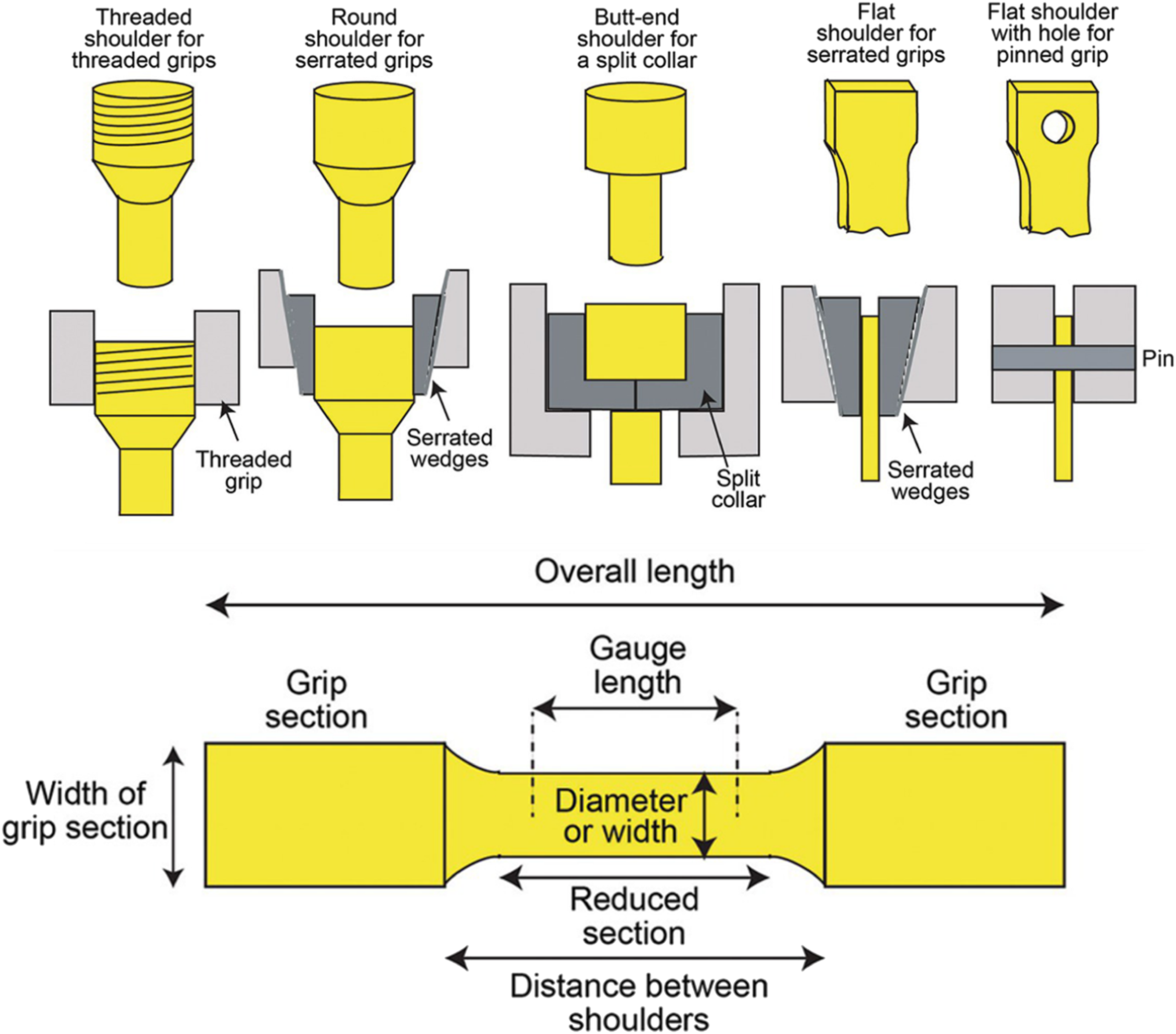
For dynamic loading on composites in tension, there are few investigations and even fewer results available due in a large part to the challenges and specialized equipment.³ To start, consider all three requirements for a successful test: tensile loading, composite material specimen, and dynamic loading conditions. With the exception of compression testing inducing an unstable deformation mechanism especially for slender specimens (height/radius aspect ratios >>1 that limit applications of confined compression testing due to induced buckling modes), testing under tension is in general more challenging. Under tension, wedges, grips or pinned connections are required to prevent the material from slipping away from the loading mechanism whereas in compression, once induced structural instability is avoided, simply requires two flat parallel surfaces to move towards each other. See Figure 1.

Figure 1.

Various grip strategies for tension loading and common terminology for specimen in tension loading.⁴

Composite materials are not as durable in directions perpendicular to the fiber orientation and, despite having high specific strength parallel to the fibers, they are not readily machined without compromising strength. When tension testing composite coupon specimens, typically flat specimens are used with a necked region and additional layered tabs to reinforce the grip section (Figures 2–3). Drilling holes is also possible in the grips to mechanically pin the specimen to the loading machines although this usually results in failure of the specimen around the hole as opposed to the gage area within the reduced section. For both fastening options, since composites do not have high crushing strength perpendicular to the fiber placement, grip pressure must be balanced to avoid slippage under loading or crushing resulting in premature failure.

Figure 2.

Unsuccessful composite tension test due to failure outside of the reduced section; reproduced from.⁵

Figure 3.

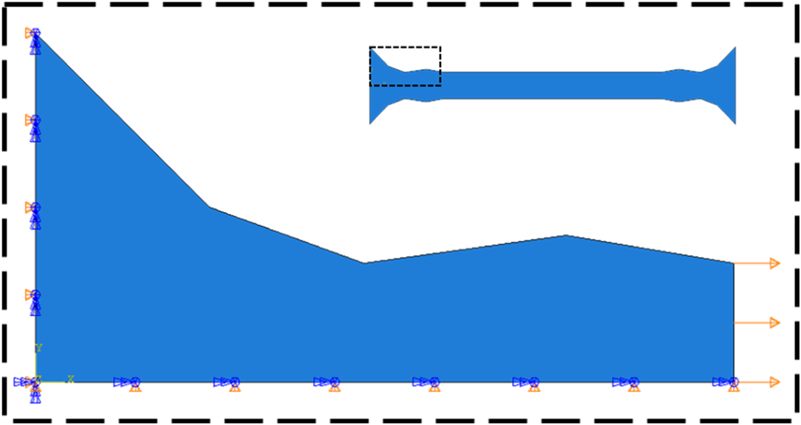
Details of an arbitrary quarter symmetric geometry in the necking-tab region and BC conditions used in ABAQUS as an example of the FEA pre-process for generating the database to input the artificial neural network.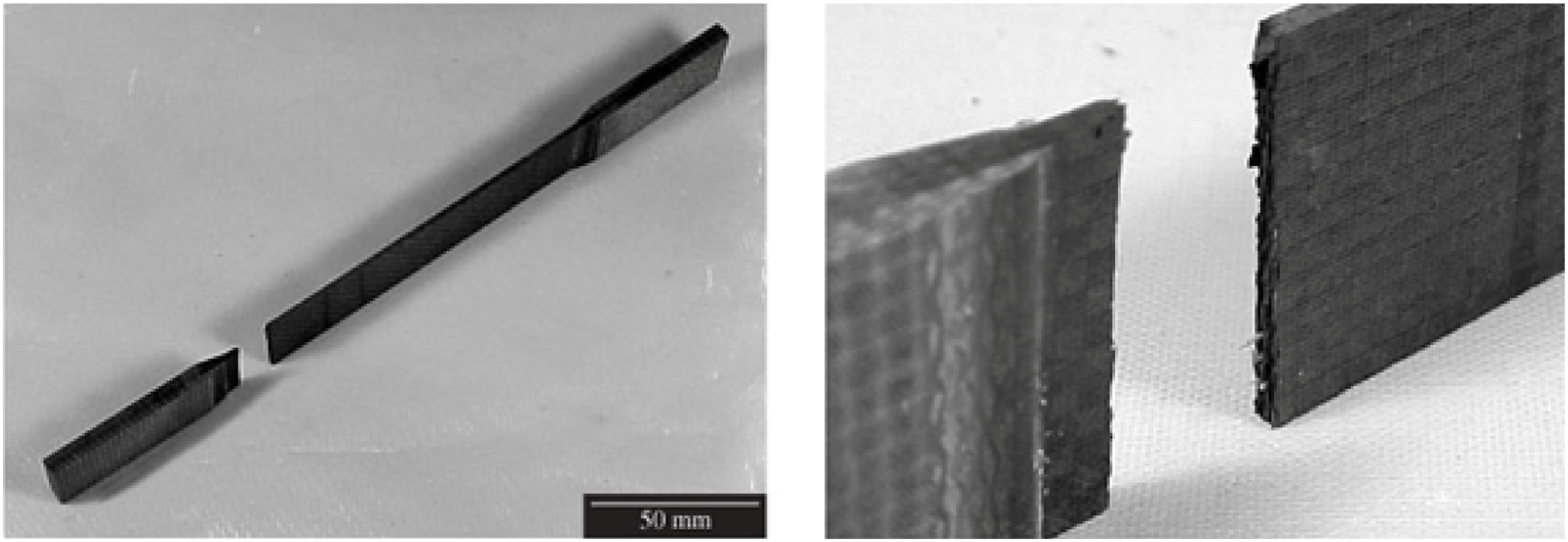

Finally, in dynamic testing, these same issues are magnified since the grips are suddenly pulled apart and the kinematic friction is lower than static friction. Composite specimens are susceptible to failure near the grip section (Figure 3). By comparison, metal specimens are easier to test in tension since there are more ways to grip them including mechanically threading the part into the fixtures (Figure 1).

Provided that the test conditions are achievable (tension, dynamic, composite) the specimen itself must be optimized for minimizing failure outside of the reduced section since homogeneous stress field is preferrable to determine not only the strength but also the material constants. As standards are not present for this, and since the composites have more complex failure mechanisms, a new approach is proposed to facilitate this experimental and numerical process. The purpose of this investigation is to demonstrate Machine Learning (ML) for specimen geometry optimization to minimize stress concentrators in unwanted regions. This will be achieved by predicting the local damage on the boundaries of a composite laminate for a range of fiber orientations and profile geometries under tension.

In order to identify and quantify possible non-statistical factors for the premature and off-centered failure mechanisms observed, FEA to simulate a quarter symmetric composite lamina and a portion of the grip section in stress-free conditions, using the mechanical properties from Table 1 in ABAQUS. Given the morphology and boundary conditions (BC) of the test, the stress field can be entirely contained in the lamina plane, thus the problem is efficiently reduced to plane stress considering only the cross-section geometry of the grip section until the area reduction of the gage section. Figure 3 shows the BC simulating tension in ABAQUS. The resulting principal stress field and Hashin damage are shown in Figures 4 and 5, respectively.

Table 1.

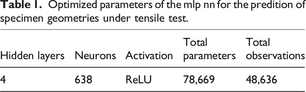
Optimized parameters of the mlp nn for the predition of specimen geometries under tensile test.

Hidden layers	Neurons	Activation	Total parameters	Total observations
4	638	ReLU	78,669	48,636

Figure 4.

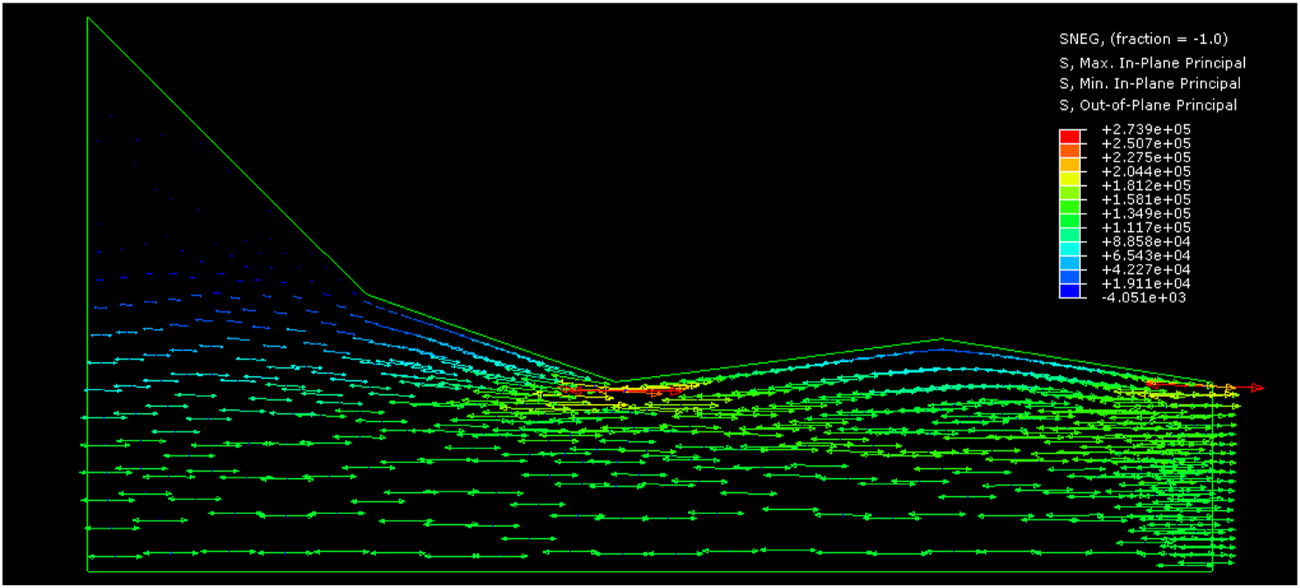
Results from FEA ABAQUS showing the principal stress distribution in the simulated composite lamina in the necking-tab region.

Figure 5.

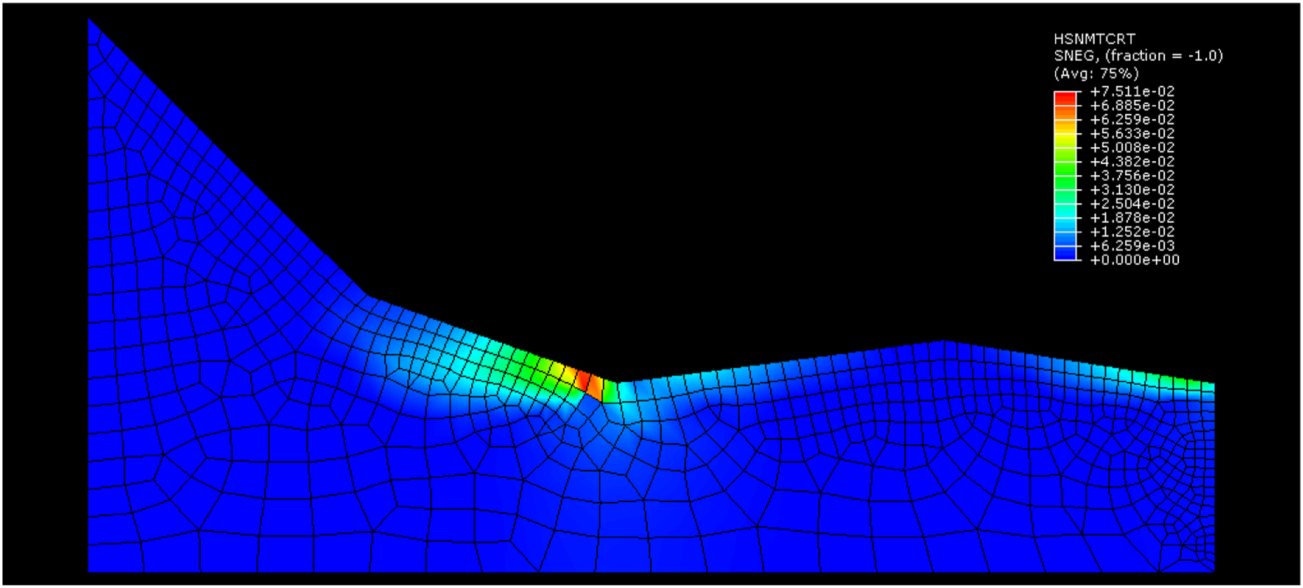
Results from FEA ABAQUS showing the Hashin damage distribution in the quarter lamina simulating the necking-tab region.

These results indicate the region in the vicinity of the grips is more likely to cause the onset of damage in the specimen due to stress concentration in the necking regions. Since the stress concentration is expected to be the dominant factor for failure under tension leading to brittle cracking and catastrophic failure, this research aims to examine the topological optimization of the necking region connecting the grip and gage regions of the specimen (treating the tab and specimen as a single component). The investigation uses a combination of two powerful tools (FEA and ML) to improve current FEA prediction processes, topological optimization and computational speed, performance and efficiency.

Literature review

Dynamic tension testing on coupon specimens in a laboratory environment typically involves smaller-sized geometries, on the order of millimeters since the speeds (and forces) involved are lower.⁶ For a 10 mm long specimen in uniaxial loading, the test rig (either tension or compression) would need to be moving at 10 m/s in order to provide an initial strain rate of 1000 s⁻¹, where the loading velocity divided by gage length. Moving to larger specimens which are often necessary to install strain gages and/or span the meso/macro-scale behavior (on the order of a few centimeters in length) and accounting for specimen shape since high-speed dynamic loads often force stress concentrations in unwanted regions (e.g. near the ends and not in the gage region) requires revisiting the test methodology. Developing new protocols with validated solutions is both costly and time consuming. Machine learning is a powerful new tool that may have the solution to this problem.⁷ ML is a subset of artificial intelligence, devised to use computational power along with statistical methods and optimization algorithms to bolster the traditional human-based capabilities in the engineering environments. This allows both ML to achieve the goals of the project and investigations more quickly and efficiently. Multiple studies demonstrate the importance of implementing ML into traditionally laborious works, such as imaging and pattern identification and recognition, non-destructive testing, and topological optimization⁸; the latter being a traditional method implemented for structural design purposes. Topological optimization has been studied for the last 35 years,^9–11 taking advantage of the finite element methods involving generally manual iterative processes that extend beyond the current state of ML automatization times especially due to the development of Deep Neural Networks using Deep Learning Strategies. The current state of the art justifies the use of ML in topological optimization because of the significant reduction in computation time for obtaining quantitatively equitable solutions to a given structural problem. The methods employed by ML include the Physics Informed Neural Network for higher accuracy results, which is essentially an additional constraint for the results obtained from the Artificial Neural Network (ANN) to guarantee the solution is physically meaningful. This employs the usage of the partial differential equations of the phenomenon observed or simulated in traditional FEA. Research has been conducted especially during the last decade in this subfield of artificial intelligence to implement ML strategies into the topological optimization and results are able to obtain time reductions of several orders of magnitude.^12–17 Recently generated extrapolation experiments have even obtained geometries never seen before using ML.¹⁸ As a corollary, it is possible then to use ML to design tension tests for composite materials that would prevent premature failure and failure outside the studied regions of interest, thereby reducing the setup times and number of replicate tests.

Therefore, using this technique it should be possible to design the ideal composite coupon specimens for tension testing at virtually any lab-achievable loading rate providing a higher time-efficiency and with less computational expensive than other current numerical method.

Materials and methods

The ML proof of concept implemented in this investigation must first demonstrate the capabilities of a Deep Learning Neural Network in predicting the BC of a structural plane stress conditions. The FEA model uses 2D shell SR4 elements since under simulated tensile conditions the out of plane stress components $σ_{x z} ≅ σ_{y z} ≅ σ_{z z} ≅ 0$ are negligible. For this strategy to be successful, the ANN extrapolation of a given input to the system needs to be trained. Here training refers to the process in which the ML approach uses database information from previous, similar scenarios in order to cast the validation and prediction results/outcome. Figure 6 shows a dense ANN diagram, consisting of the inputs/features, biases, weights, and outcome. These elements are classified based on input, hidden and output layers in which every stack of layers is a computation of weights/coefficients plus biases that are composed into an activation function which is again composed into every hidden layer before the process reaches the output layer. The gradient descent computes the so-called back propagation which is the iterative process optimizing the constants of the modals increasing the importance/magnitude of the weights of certain inputs mimicking the way a real neural system work in the brain. This process then efficiently selects the most sensitive and significant inputs to generate an accurate formulation model of the experimental observations.

Figure 6.

Representation of a multi-perceptron artificial neural network.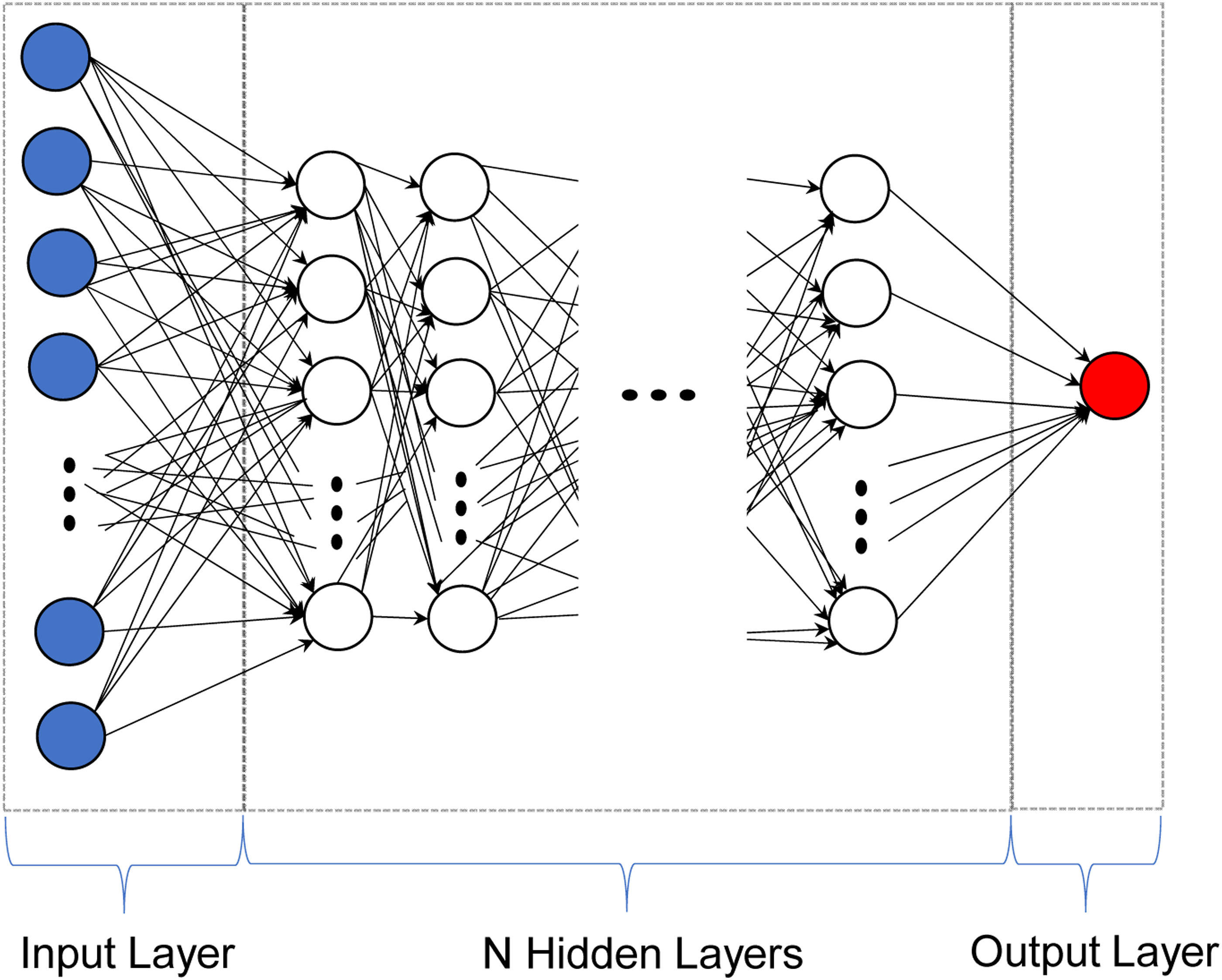

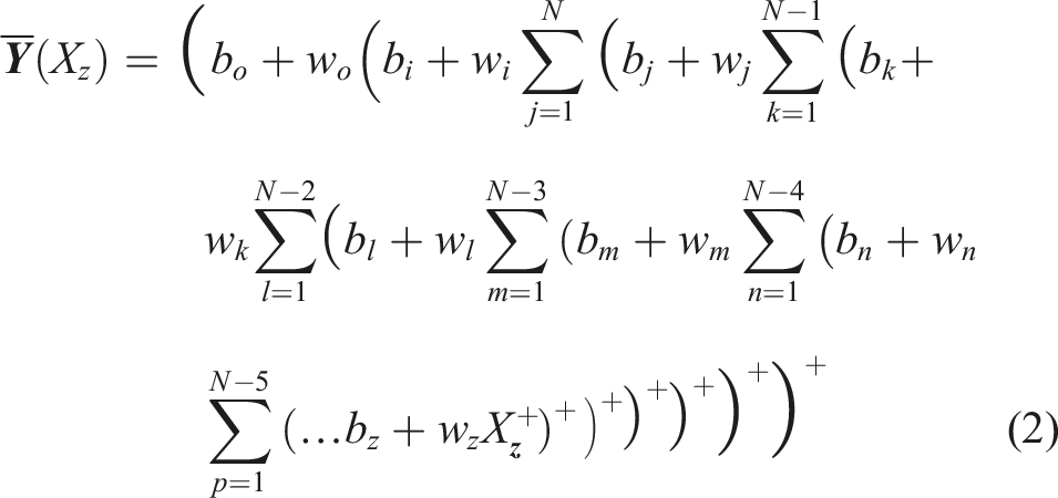
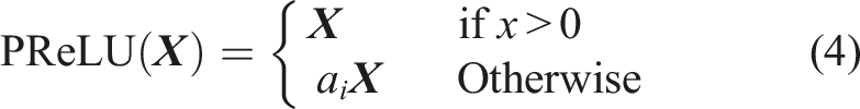
In this case a Multi-Perceptron (MLP) ANN is implemented and configured to predict outcomes using the provided inputs. This is the validation process and once the MLP parameters are tuned using a validation dataset, the model is tested using never before seen output. This testing accuracy is the deciding parameter for the model, and in the present study, the coefficient of determination R² is used. The model generates a mathematical function of the inputs combining weights and biases composed into an activation function that becomes the model for the output. We can imagine the process of composing a linear activation function such as the Rectifier Linear Unit (ReLU) equation (1) in which only the positive part of the input is considered. This results in the mathematical model of the thN^th layer ANN that can be described by equation (2). 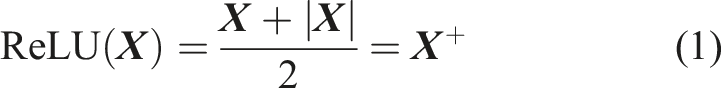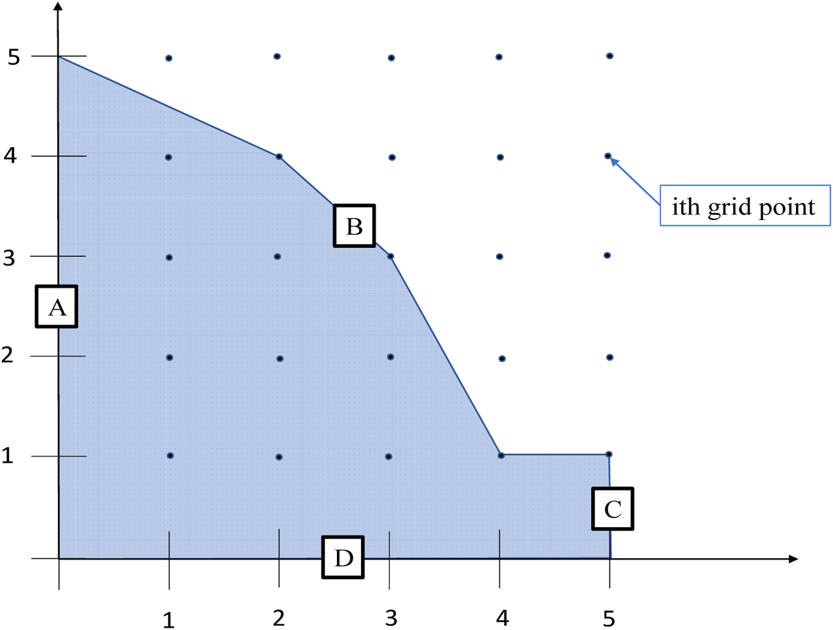Variables $b_{i}$ and $w_{i}$ represent the total parameters used in the model of the output that is, biases and weights at every neuron, respectively. Equation (2) thus shows qualitatively the resulting composition of the estimated output model $\bar{Y}$ using the rectifier is linear with respect the input array $X$ .

ReLU (X) = \frac{X + | X |}{2} = X^{+}

(1)

\bar{Y} (X_{z}) = {(b_{o} + w_{o} {(b_{i} + w_{i} \sum_{j = 1}^{N} {(b_{j} + w_{j} \sum_{k = 1}^{N - 1} {(b_{k} + w_{k} {\sum_{l = 1}^{N - 2} (b_{l} + w_{l} \sum_{m = 1}^{N - 3} (b_{m} + w_{m} \sum_{n = 1}^{N - 4} (b_{n} + w_{n} \sum_{p = 1}^{N - 5} {(\dots b_{z} + w_{z} X_{z}^{+})}^{+})}^{+})}^{+})}^{+})}^{+})}^{+}

(2)

Similar activation functions are considered in this investigation, such as the Exponential Linear Unit (ELU) and the Parametric ReLU (PReLU), Eq. (4) and Eq. (5) respectively, where the term

a_{i}

is a constant added in each activation.

ELU (X) = {\begin{cases} X if x > 0 \\ a_{i} (e^{X} - 1) Otherwise \end{cases}

(3)

PReLU (X) = {\begin{cases} X if x > 0 \\ a_{i} X Otherwise \end{cases}

(4)

The ANN then uses stochastic gradient descent to optimize the difference in between the generated function and the desired output, minimizing a loss function which is the difference between these two datasets (i.e., the input data set generated at every step of the iteration method and the known outcome until the tolerance criteria is met). The stop conditions generally are residual tolerances or iteration limit set on both. The ANN fit to the known dataset and the validation set (a smaller set to verify the prediction performance) are both based on predefined values of Relative Root Mean Squared Error (RRMSE) for the fit and validation datasets, also defined as loss. The tolerance stop-criteria used was an RRMSE value of 1% for the fitting process (model and the training set), while a value of 5% was established for the validation (a small prediction set). For this proof of concept, the inputs are internal traction vectors $t_{i} = σ n_{i}$ under tension of different simulated necking-tab regions, quarter symmetry, displayed with the respective BC and profile geometry shape using a function $f (x)$ where axial coordinate $x$ is indicated in Figure 7. The traction provides a 2D vector containing the components of the stress $σ_{x x}$ , $σ_{y y}$ and $σ_{x y}$ in the regions A, B, C and D shown in Figure 8, illustrating the simulated necking region of the specimens under tension. This synthetic data is obtained using ABAQUS Standard generating a database for the different numerical simulation of the different geometries. Each geometry is produced by applying permutations of linear segments connected in a 5 × 5 square grid of points shown in Figure 9. Since the size of the database is a trade-off between computational efficiency for the FEA software and the input database to feed the ML ANN, a compromise in the number of geometries resulted in the final 1134 set of different profiles.

Figure 7.

Representation of the quarter sectioning of the necking-tab region to be generated for the FEA simulations of the composite specimen.

Figure 8.

Quarter section geometry of specimen with BC coded as follows: (left) in blue is a 2% uniformly distributed extension displacement; (bottom) in green is a limit on vertical displacement due to the axis of symmetry; (right) in red is the restraint in the horizontal displacement where height $h$ is trained and predicted. The top region in black (non-linear geometry of the specimen’s edge) is trained with the profiles $f (x)$ to be predicted.

Figure 9.

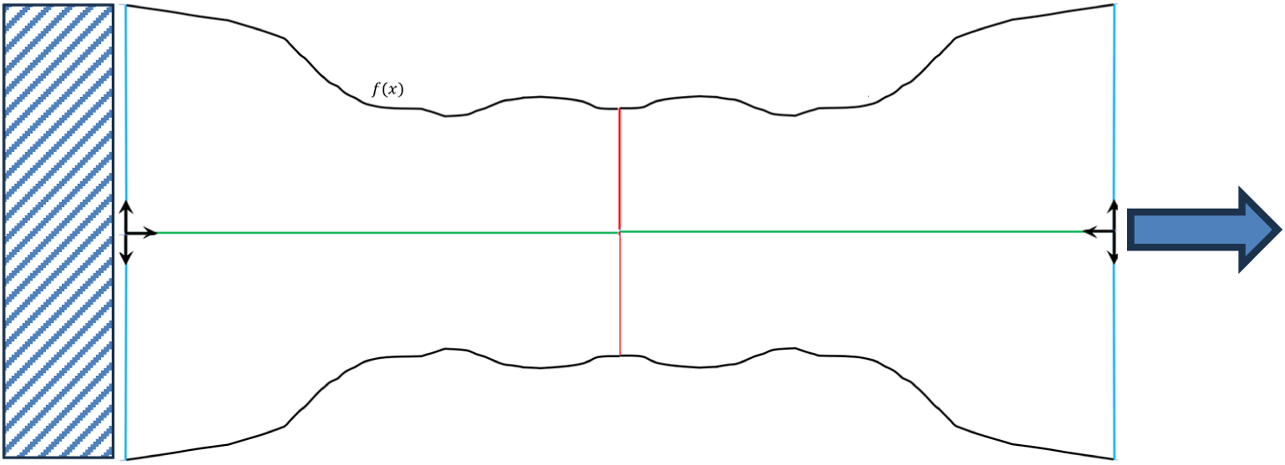
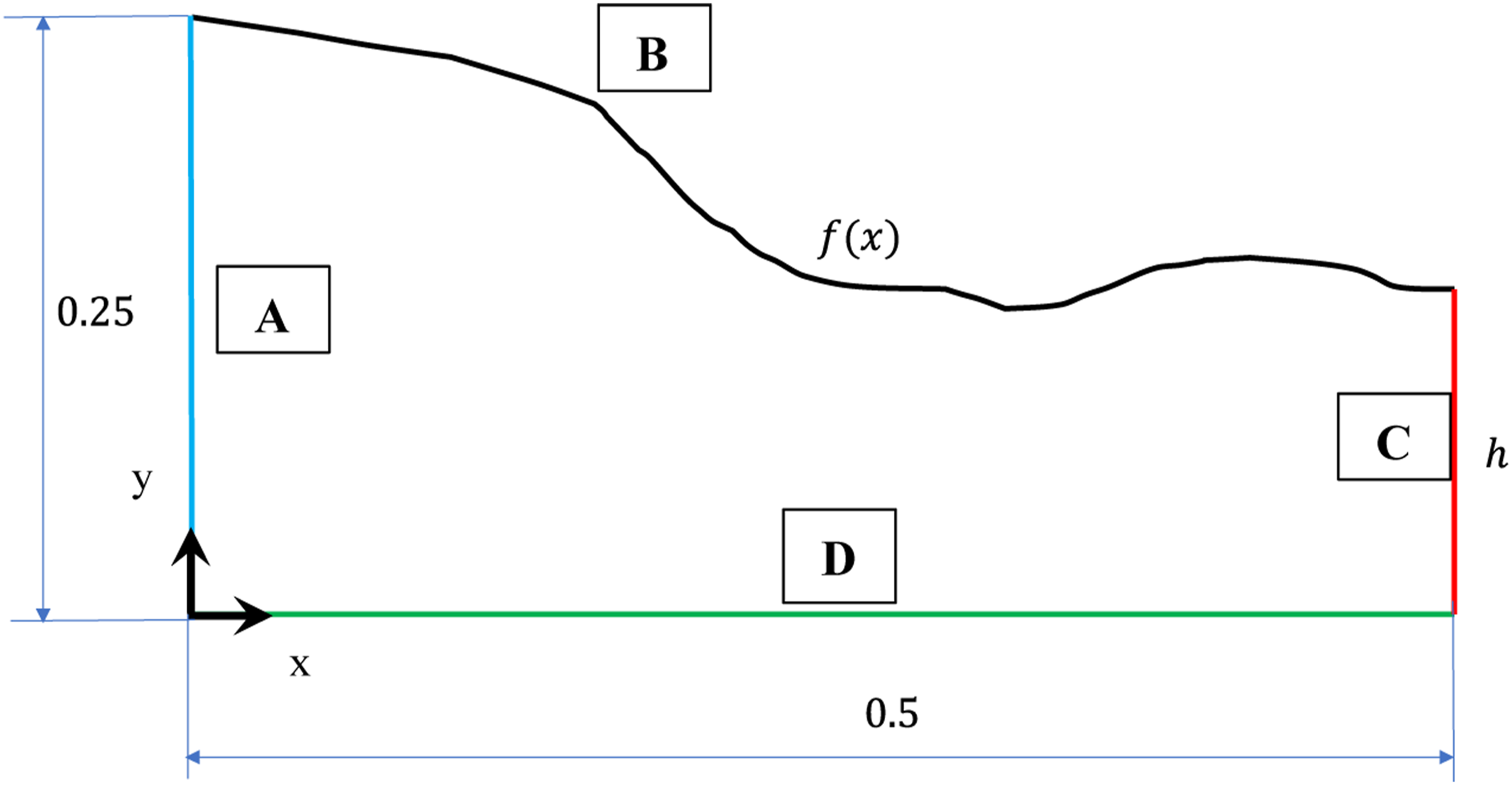
Quarter section geometry of specimen showing the method used to generate the $5^{5}$ different profile shapes using permutation of equally spaced the points connected to the 5 × 5 grid.

The design envelope has been selected to mimic a tension specimen that cannot stretch at $x = 0$ (support) with a horizontal displacement imposed at $x = 0.5$ . There were no constraints imposed on the $f (x)$ curve, that is, stress free region, with only first and last points of this curve sharing BCs. Tabs are part of the geometry generated since the simulations include the necking-tab region as one single part. This effectively merges the stress-free tab region and the specimen at the axis of symmetry and uses the same material.

For a quarter of symmetry ABAQUS simulation, this is equivalent to imposing a fixed condition on the edge ( $x = 0.5$ ) and the stretching displacement on the edge ( $x = 0$ ) in Figure 8. The arbitrary curve represents the unknown profile of the specimen. The datasets introduced in the ANN contains the desired output array of the different specimen’s profiles as a piece-wise function of the horizontal position, that is, $f (x)$ , and the traction vectors result in the edge regions A and C from Figure 8.

Results and discussion

The FEA results are the stress tensor components extracted from the traction vector along regions A and C in Figure 8 and shown for a singled-out geometry in Figure 10. These results are the inputs to train the ML ANN to provide a prediction of the profile geometries given only their stress distribution. The results obtained in the validation stage of this ANN are summarized in Table 1 consisting of the prediction of 10 different profiles displayed in Figure 11 resulting in a predicted accuracy of R² = 0.98. Here the ANN is composed of a total of six layers, #1 is the input layer, #2-5 are the hidden dense layers accounting for a total of 638 neurons, the last #6 layer is the output layer which renders the final result as output. All of these neurons, composition of biases, and weights compose the ReLU activation function for a total of 78,669 parameters that define the model for prediction and the geometries based on the 48,636 input stress points from every region in Figure 8.

Figure 10.

Stress components on the boundaries of the specimen A and C (Top), used as input for the ANN to predict the specimen’s geometry (Bottom).

Figure 11.

Actual and predicted of 10 specimen geometries obtained after the MLP ANN model concludes the fitting/training process, which rendered a R² = 0.98 in predicted accuracy. Blue is the original geometry and green is the predicted geometry.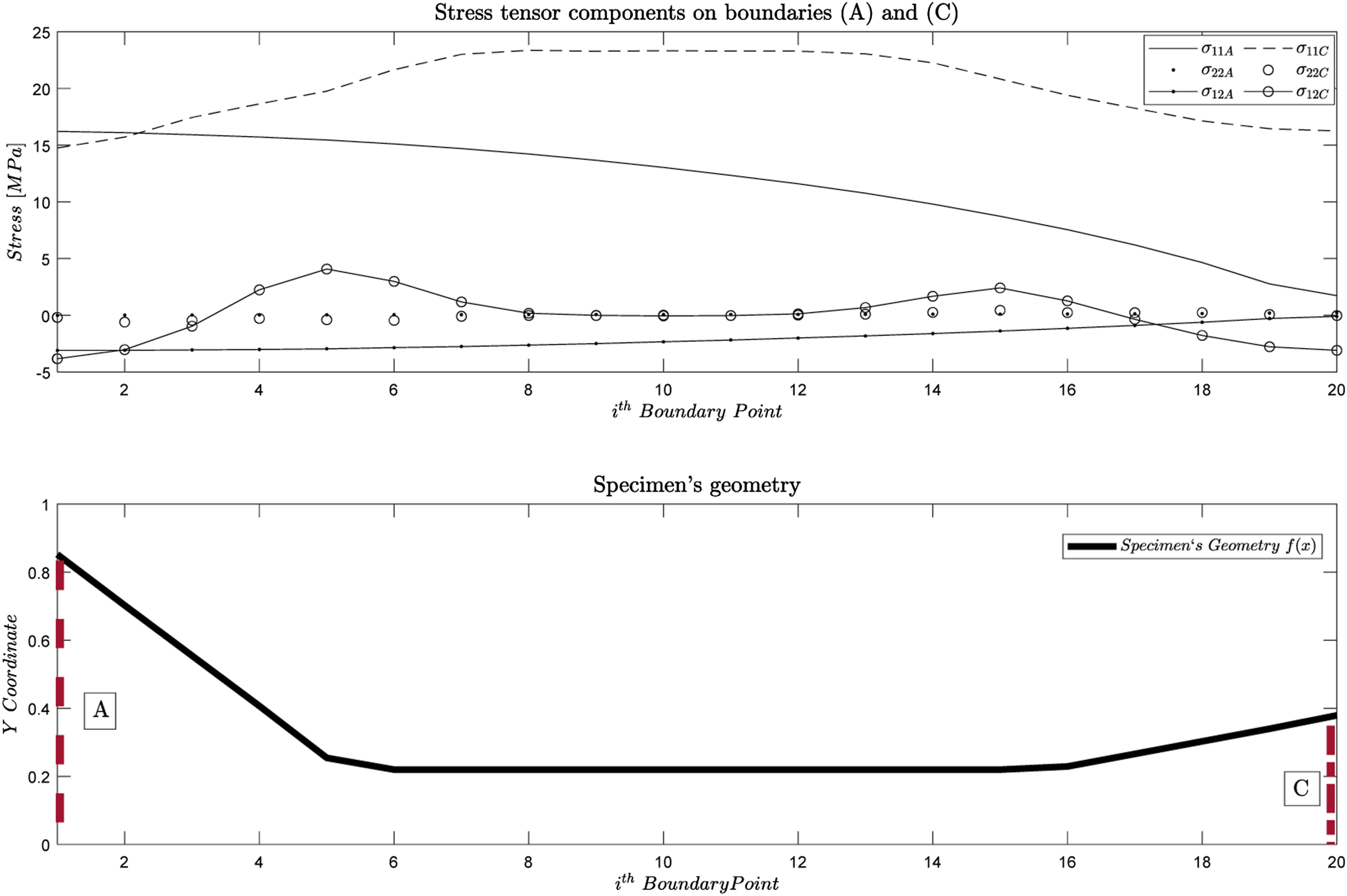

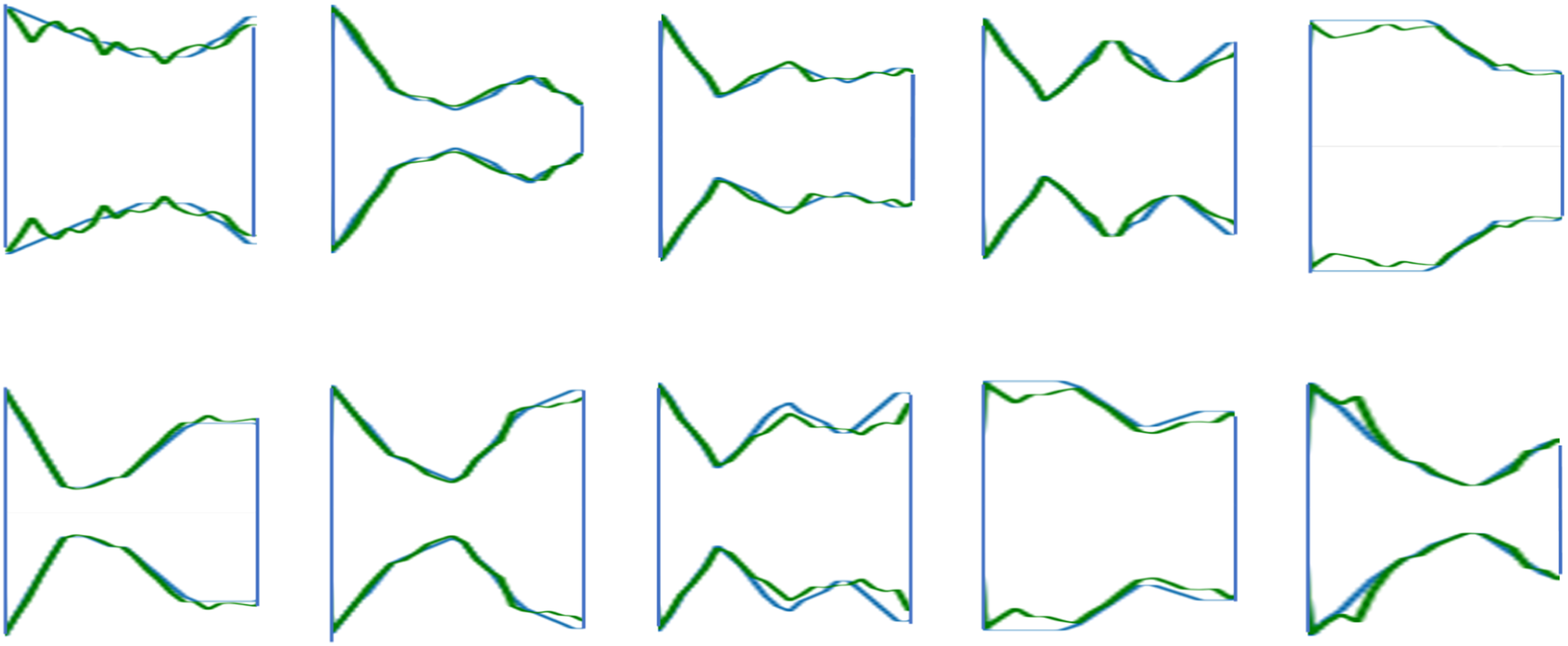
Therefore, it can be concluded the training and validation/prediction process are deemed successful and thus the model reliably predicts the specimen’s profiles. It should be emphasized that the model does not know the geometry of the specimen to be predicted as this remains unseen in the validation and test datasets. The model is instead determining their shapes only with the information of the stress components from the traction vector.

With the predicted results validating the proof of concept, the next step is using the same prediction capabilities on the geometric parameters of composite materials. Both fiber orientation and geometry of the composite can be optimized for these transient stresses while complying with the established requirements of both design and structural limits. Furthermore, the advantage of this ML and topologic optimization is meshless as compared to the traditional numerical simulations, delivering high quality results with time and computational advantages, including in the time integration spare process. Since there is no need for time integration schemes required of explicit analysis, realistic time savings in the order of 10,000:1 are attainable using this methodology. No iterations in the ANN are necessary when the same training data set is used to predict the outcome. Here geometry prediction will be combined with internal stress and damage prediction of composite specimens (similar to the visualization in Figure 10). Finite element results for a non-optimized transient equivalent stress wave are shown in Figure 12 indicating the areas of high stress within a composite with two fiber orientations.

Figure 12.

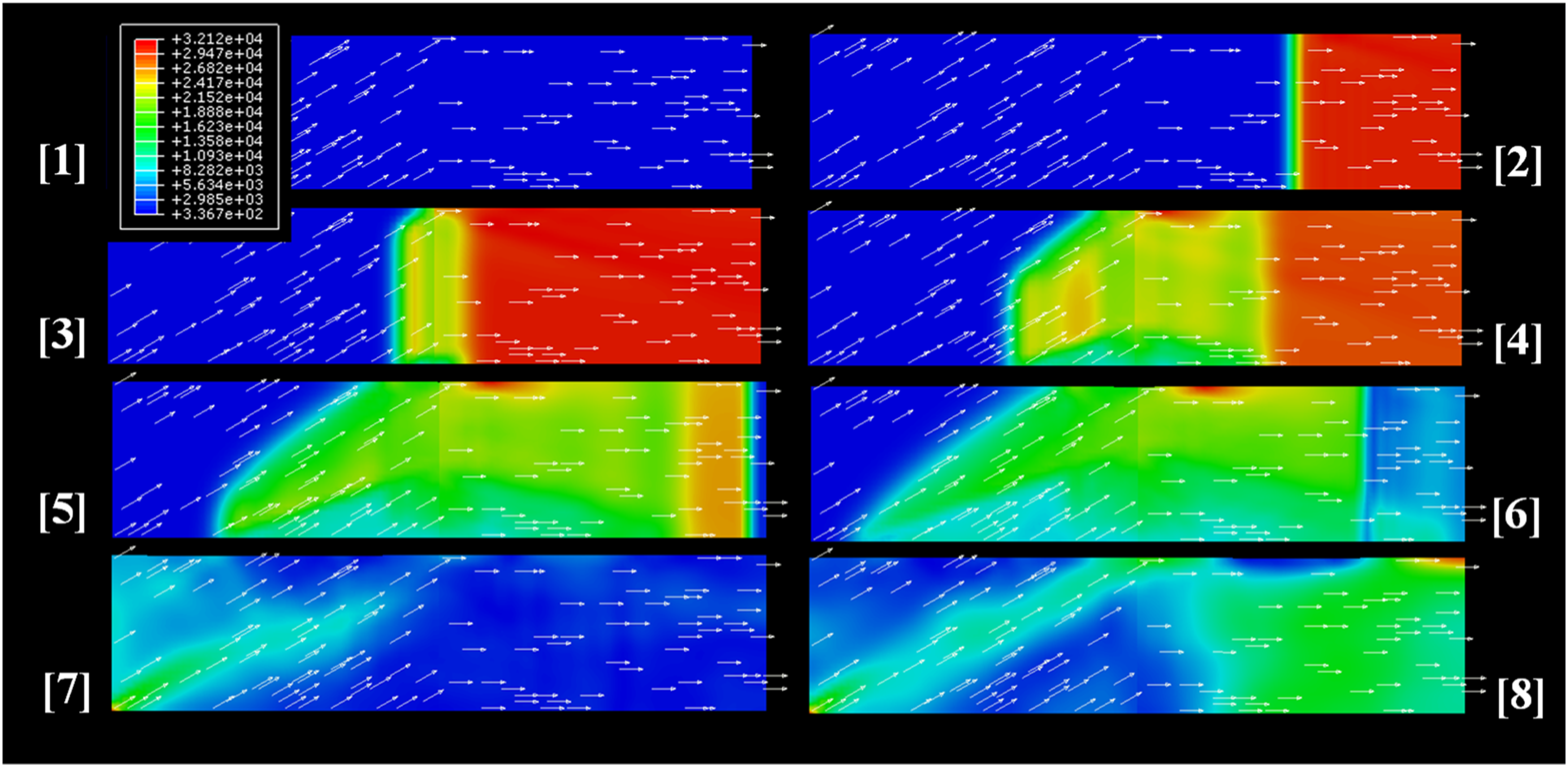
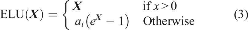
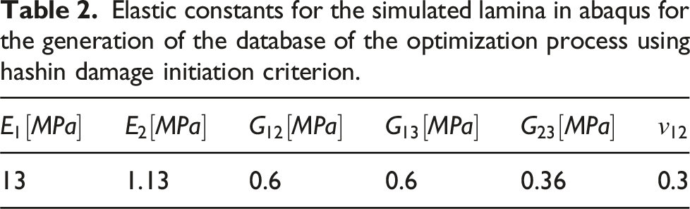
Stress distribution through a composite with two different fiber orientations during a dynamic tension test using FE ABAQUS, sequence times corresponding to [1] 0 ms, [2] 3 ms, [3] 7 ms, [4] 10 ms, [5] 12 ms, [6] 25 ms, [7] 44 ms, [8] 78 ms.

The database of the simulations generated via ABAQUS consists of 320 orthotropic laminated grip section geometries with properties shown in Table 2 mechanical. Each geometry used a denser mesh (120 points per geometry compared to the 5 × 5 mesh from the proof of concept) in order to obtain more local points on the larger boundary regions A, B and C, plus the fiber orientation.

Table 2.

Elastic constants for the simulated lamina in abaqus for the generation of the database of the optimization process using hashin damage initiation criterion.

$E_{1} [M P a]$	$E_{2} [M P a]$	$G_{12} [M P a]$	$G_{13} [M P a]$	$G_{23} [M P a]$	$ν_{12}$
13	1.13	0.6	0.6	0.36	0.3

The damage initiation criterion used was the Hashin damage¹⁹ for plane stress equations (5)–(8) where the respective lamina strength properties are in Table 3, and the damage evolution criterion based on energy is defined with the material constants in Table 4. The results BC applied for these simulations are identical to the ones described in the isotropic material proof of concept in Figure 8.

Table 3.

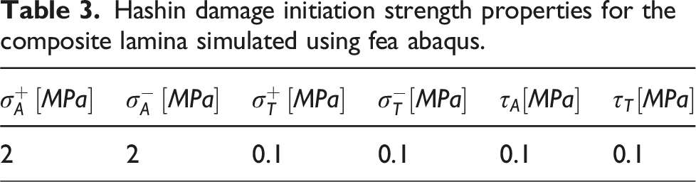
Hashin damage initiation strength properties for the composite lamina simulated using fea abaqus.

$σ_{A}^{+} [M P a]$	$σ_{A}^{-} [M P a]$	$σ_{T}^{+} [M P a]$	$σ_{T}^{-} [M P a]$	$τ_{A} [M P a]$	$τ_{T} [M P a]$
2	2	0.1	0.1	0.1	0.1

Table 4.

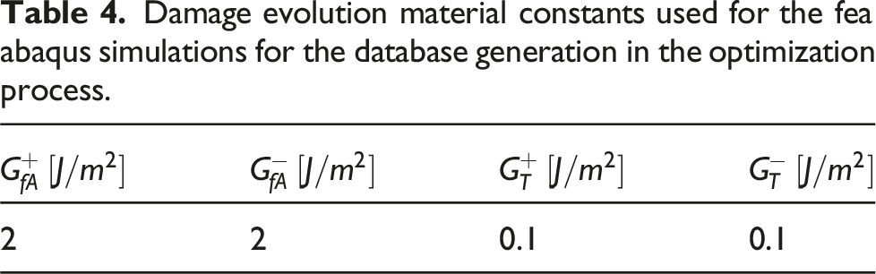
Damage evolution material constants used for the fea abaqus simulations for the database generation in the optimization process.

$G_{f A}^{+} [J / m^{2}]$	$G_{f A}^{-} [J / m^{2}]$	$G_{T}^{+} [J / m^{2}]$	$G_{T}^{-} [J / m^{2}]$
2	2	0.1	0.1

For tensile failure mode: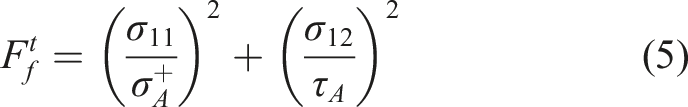

F_{f}^{t} = {(\frac{σ_{11}}{σ_{A}^{+}})}^{2} + {(\frac{σ_{12}}{τ_{A}})}^{2}

(5)

Compressive Fiber Mode: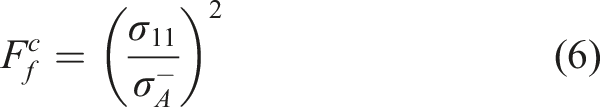

F_{f}^{c} = {(\frac{σ_{11}}{σ_{A}^{-}})}^{2}

(6)

Matrix Tension: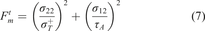

F_{m}^{t} = {(\frac{σ_{22}}{σ_{T}^{+}})}^{2} + {(\frac{σ_{12}}{τ_{A}})}^{2}

(7)

Matrix Compression: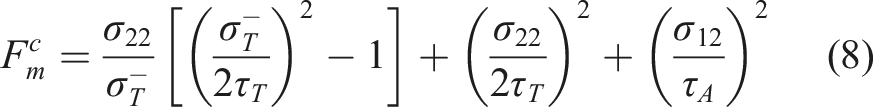

F_{m}^{c} = \frac{σ_{22}}{σ_{T}^{-}} [{(\frac{σ_{T}^{-}}{2 τ_{T}})}^{2} - 1] + {(\frac{σ_{22}}{2 τ_{T}})}^{2} + {(\frac{σ_{12}}{τ_{A}})}^{2}

(8)

Where the terms in the damage initiation criterion are defined as¹⁹:

$σ_{A}^{+}$ = tensile failure stress in fiber direction

$σ_{A}^{-}$ = compressive failure stress in fiber direction (absolute value)

$σ_{T}^{+}$ = tensile failure stress transverse to fiber direction

$σ_{T}^{-}$ = compressive failure stress transverse to fiber direction (absolute value)

$τ_{T}$ = transverse failure shear

$τ_{A}$ = axial failure shear

Where the terms are respectively:

$G_{f A}^{+}$ = Longitudinal tensile fracture energy

$G_{f A}^{-}$ = Longitudinal compressive fracture energy

$G_{T}^{+}$ = Transverse tensile fracture energy

$G_{T}^{-}$ = Transverse compressive fracture energy

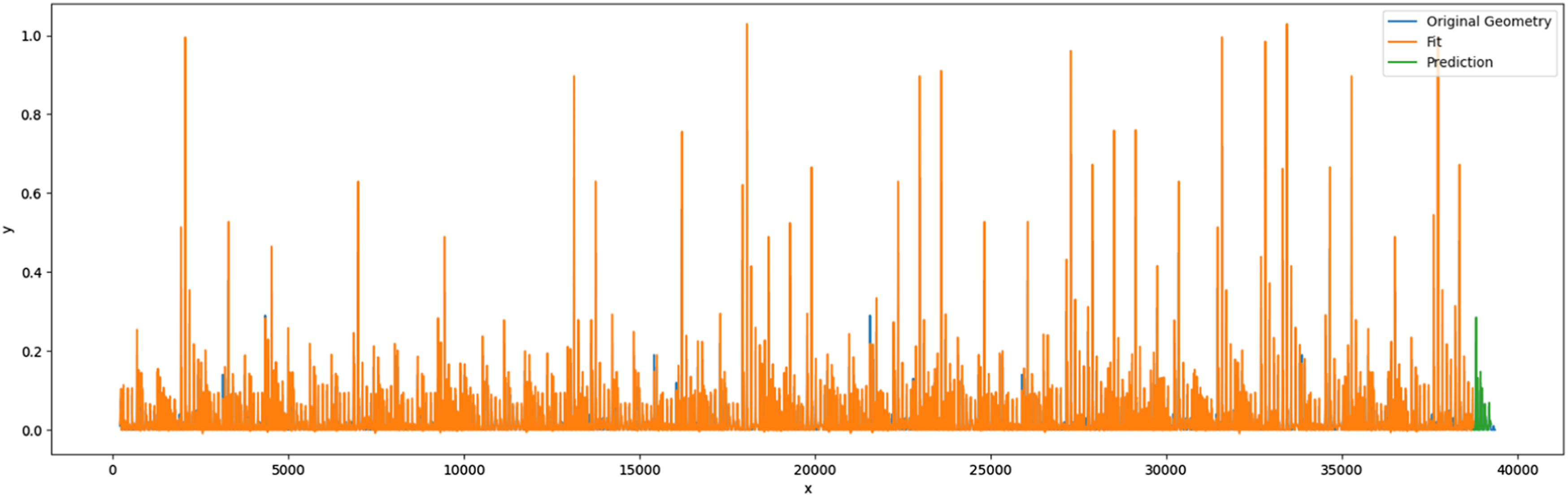
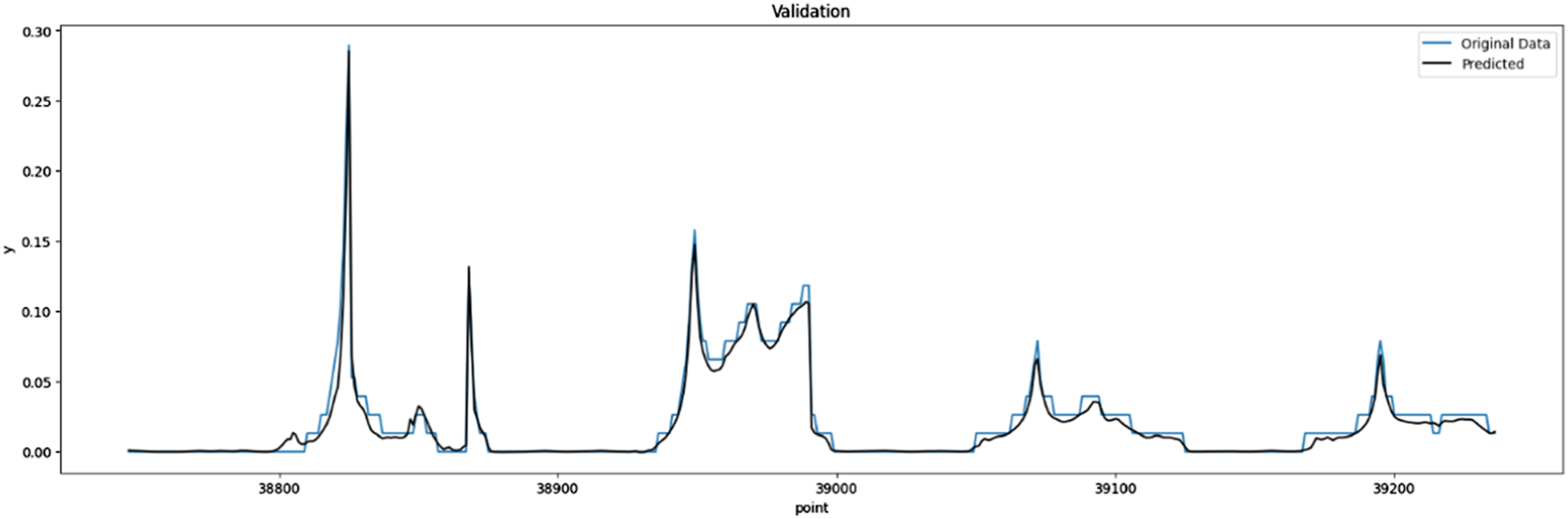
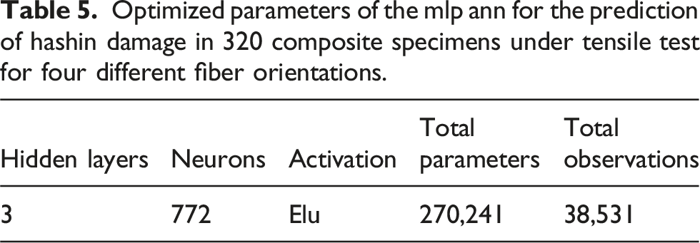
This approach is complemented with the addition of the fiber orientation as a variable since the goal is to predict damage locally at the boundary regions A, B and C indicated in Figure 8 using unseen geometries for different fiber orientations. In this case, the input database for the ANN is grip geometries and the output to fit and model are the Hashin damage in the mentioned boundary regions. Both are shown in Figure 13 using matrix damage as output. Then by combining the prediction capabilities of both methods, that is, using ML to predict stresses and damage in composites and to topologically optimize the designs, we can thus set the initial steps to design improved/optimized coupon composite specimens for dynamic tensile testing. Results from the damage fit data are shown in Figure 14. The local predicted damage in the composite for four different fiber orientations is displayed in Figure 15. Details for the ANN are summarized in Table 5. The NN is composed of a total of five layers, #1 is the input layer, #2-4 are the hidden dense layers accounting for a total of 772 neurons, the last #5 layer is the output layer which renders the final result as output. All of these neurons, composition of biases, and weights compose the Elu activation function for a total of 270,241 parameters that define the model for prediction and the geometries based on the 38,531 input stress points from every region provided in Figure 8.

Figure 13.

Top. Results from the FEA of the local damage on the necking-tab region of the simulated specimens on the boundary regions highlighted A, B and C. Bottom. Geometry of the quarter sectioned necking-tab region of the simulated composite specimen.

Figure 14.

Results from the training process of the ANN using the Hashin damage criterion as output for a total of 320 FEA simulations using ABAQUS of composite coupon specimen geometries, and specimen and fiber orientations as inputs. Horizontal axis represents the boundary point on the regions A, B and C whereas the vertical axis represents the local damage on the respective boundary point.

Figure 15.

Validation results of the local Hashin damage criterion in the colored highlighted regions from Figure 8 using ANN. (Blue curve) shows original FEA predicted damage, (black curve) shows the predicted local damage in the exact same regions with a 97% accuracy of one geometry for four different fiber orientations.

Table 5.

Optimized parameters of the mlp ann for the prediction of hashin damage in 320 composite specimens under tensile test for four different fiber orientations.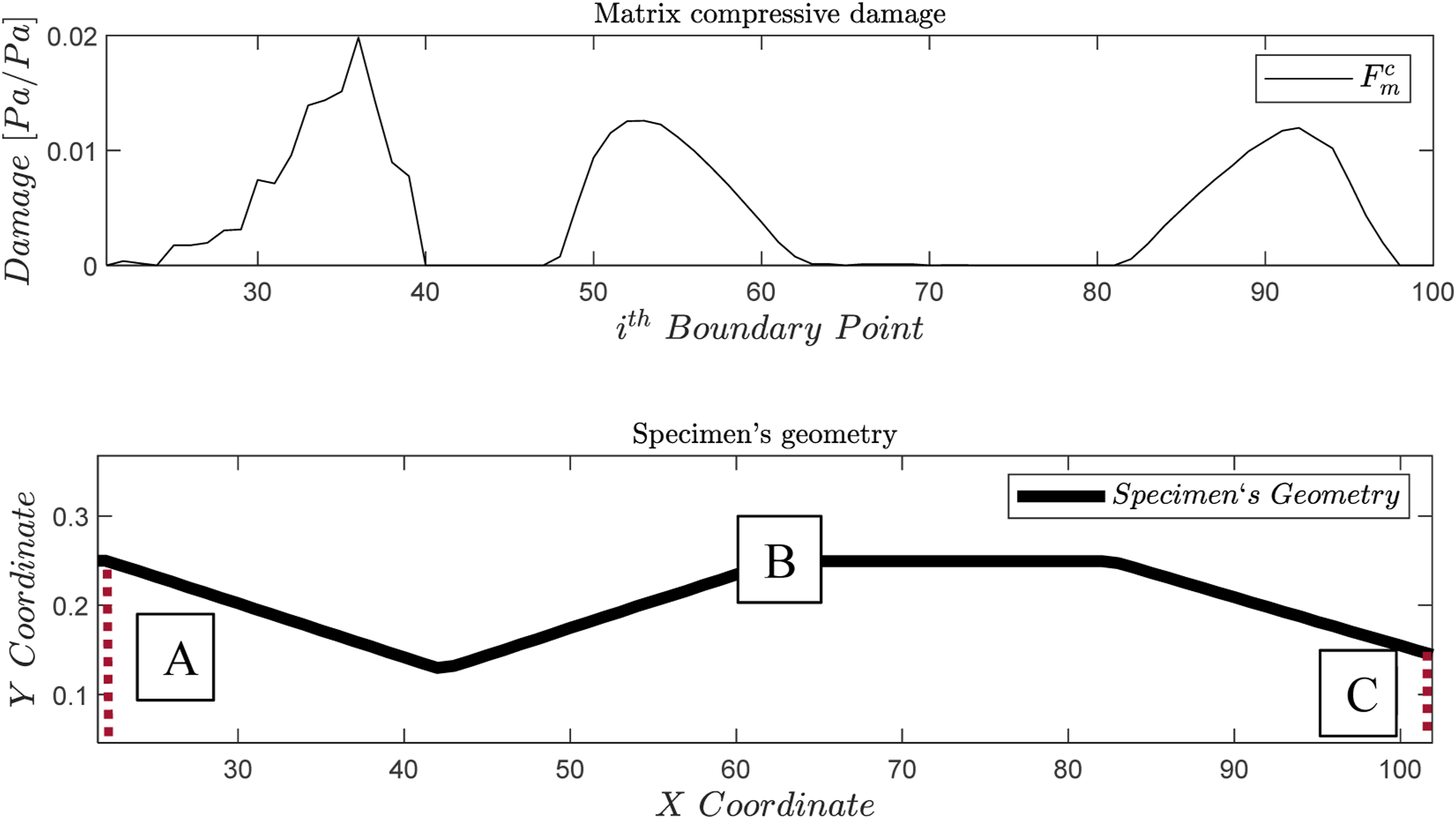

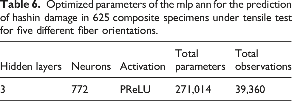
Hidden layers	Neurons	Activation	Total parameters	Total observations
3	772	Elu	270,241	38,531

The results represent one possible specimen geometry. Figure 16 provides a visualization of 625 possible tensile specimen geometries that delimit a surface map of Hashin damage in tension across all five fiber orientations (0°, 22.5°, 45°, 67.5°, 90°) using an ANN model summarized in Table 6. Parameter descriptions are similar to Table 5. These three large volume simulation tests are completed in fractions of a second which is orders of magnitude faster than even a single FEA simulation of equivalent complexity.

Figure 16.

Predicted averaged Hashin damage criterion for a total of 625 different specimen geometries with five different fiber orientations. Validation results show 99% accuracy with respect to FEA.

Table 6.

Optimized parameters of the mlp ann for the prediction of hashin damage in 625 composite specimens under tensile test for five different fiber orientations.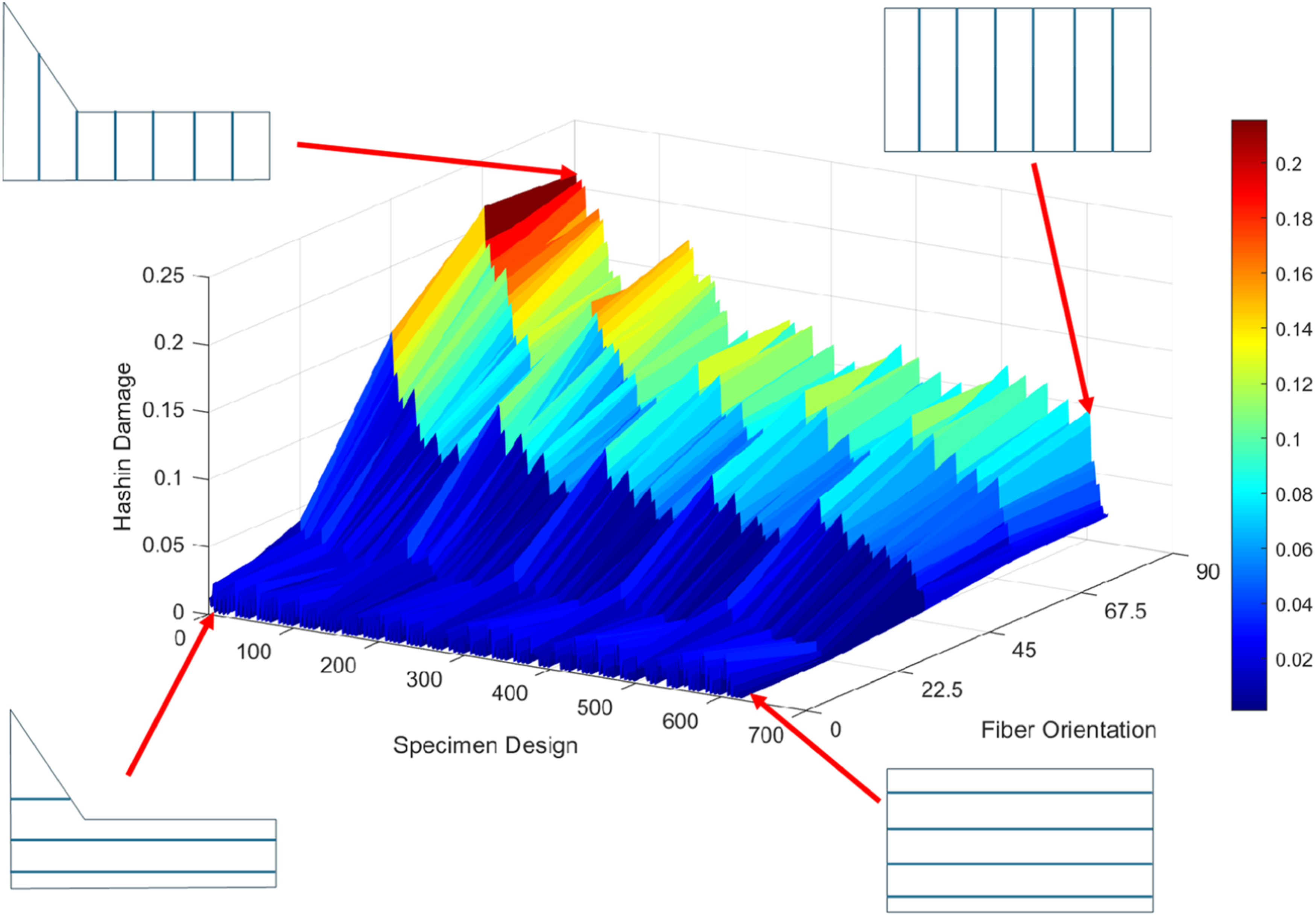

Hidden layers	Neurons	Activation	Total parameters	Total observations
3	772	PReLU	271,014	39,360

Conclusions

Developing new test protocols for dynamic loading rates on composites specimens requires significant investment in both the physical and numerical systems. Through ML, we have been able to devise a strategy that accelerates the numerical computations to optimize the specimen geometries for reducing the number of unsuccessful tests. The ideal inputs for training the ANN are the location of specimen failure and a uniformly distributed stress field in the internally studied cross section, and if correctly implemented in a ML methodology, the specific specimen geometry for a given composite fiber orientation can be computed almost instantaneously to ensure that failure will occur in the gage region of the specimens.

Footnotes

Declaration of Conflicting Interests

The author(s) declared no potential conflicts of interest with respect to the research, authorship, and/or publication of this article.

Funding

The author(s) received no financial support for the research, authorship, and/or publication of this article.

ORCID iD

Daniel Whisler

Data availability statement

Data sharing not applicable to this article as no datasets were generated or analyzed during the current study.

References

Thomsen

. CerTest: scientific foundations for a novel framework for performance validation of composite aerostructures relying less on physical testing and adopting digital twinning. In: Proceedings of the 23rd International Conference on Composite Materials (ICCM23) workshop on ‘Modernising Routes to Compliance with Composite Regulations: A Journey towards Virtual Testing and Digital Twinning, Bristol, UK, August 1, 2023. Bristol Composites Institute: Bristol, UK.

ASTM International. Standards and Publications . Composite Standards. West Conshohocken, PA, USA. https://www.astm.org/products-services/standards-and-publications/standards/composite-standards.html.

Correia

Peixinho

. Static and dynamic tensile behavior of unidirectional glass/epoxy composites. Adv Mater Res 2014; 1016: 298–301. DOI: 10.4028/www.scientific.net/amr.1016.298.

Clyne

Campbell

. Testing of the plastic deformation of metals. Cambridge, England: Cambridge University Press, 2021. ISBN 978-110-894-336-9.

De Paival

JMF

Rezende

. Comparison of tensile strength of different carbon fabric reinforced epoxy composites. Mater Res 2006; 9: 83–90. DOI: 10.1590/S1516-14392006000100016.

Mohsin

MAA

Iannucci

Greenhalgh

. On the dynamic tensile Behaviour of thermoplastic composite carbon/polyamide 6.6 using split hopkinson pressure bar. Materials 2021; 14: 1653. DOI: 10.3390/ma14071653.

Gareth

Witten

Hastie

, et al. An introduction to statistical learning with applications in R. 2nd ed. New York, NY, USA: Springer, 2021. ISBN 978-1-0716-1418-1.

Shin

Kang

. Topology optimization via machine learning and deep learning: a review. J Comput Des Eng 2023; 10: 1736–1766. DOI: 10.1093/jcde/qwad072.

Bendsøe

Kikuchi

. Generating optimal topologies in structural design using a homogenization method. Comput Methods Appl Mech Eng 1988; 71: 197–224. DOI: 10.1016/0045-7825(88)90086-2.

10.

Rozvany

GIN

Zhou

Birker

. Generalized shape optimization without homogenization. Struct Optim 1992; 4: 250–252. DOI: 10.1007/BF01742754.

11.

Mlejnek

. Some aspects of the genesis of structures. Struct Optim 1991; 5: 64–69. DOI: 10.1007/BF01744697.

12.

Almasri

Bettebghor

Ababsa

, et al. Shape related constraints aware generation of mechanical designs through deep convolutional GAN. Eng Appl Artif Intell 2020; 56: 18–35. DOI: 10.1080/0305215x.2022.2144847.

13.

Cang

Yao

Ren

. One-shot generation of near-optimal topology through theory-driven machine learning. Comput Aided Des 2019; 109: 12–21. DOI: 10.1016/j.cad.2018.12.008.

14.

Halle

Campanile

Hasse

. An artificial intelligence–assisted design method for topology optimization without pre-optimized training data. Appl Sci 2021; 11: 9041. DOI: 10.3390/app11199041.

15.

Keshavarzzadeh

Kirby

Narayan

. Stress-based topology optimization under uncertainty via simulation-based Gaussian process. Comput Methods Appl Mech Eng 2020; 365: 112992. DOI: 10.1016/j.cma.2020.112992.

16.

Sosnovik

Oseledets

. Neural networks for topology optimization. Russ J Numer Anal Math Model 2019; 34: 215–223. DOI: 10.1515/rnam-2019-0018.

17.

Zheng

Kumar

Kochmann

. Data-driven topology optimization of spinodoid metamaterials with seamlessly tunable anisotropy. Comput Methods Appl Mech Eng 2021; 383: 113894. DOI: 10.1016/j.cma.2021.113894.

18.

Sim

Lee

, et al. Gans and dcgans for generation of topology optimization validation curve through clustering analysis. Adv Eng Software 2021; 152: 102957. DOI: 10.1016/j.advengsoft.2020.102957.

19.

Hashin

. Failure criteria for unidirectional fiber composites. J Appl Mech 1980; 47: 329–334. DOI: 10.1115/1.3153664.

Designing optimized geometry and fiber orientation of composites for dynamic tension via artificial intelligence