Sage Journals: Discover world-class research

Abstract

Geothermal resource is a kind of crucial clean, renewable energy with high potential development and application. However, it involves great exploiting risks since it buried deep beneath the crust of the Earth. The location and depth of geothermal resources can be determined using the geophysical methods. Controlled source audio-frequency magnetotellurics (CSAMT) and transient electromagnetic method (TEM) have relatively high efficiency and robustness. In this paper, a simplified geothermal system resistivity model was established, which allowed TEM and CSAMT to differentiate target faults with various characteristics (resistivity, dip angle and width). Through a comprehensive electromagnetic exploration in Huairen County, Shanxi Province, China as an example, the performance of TEM and CSAMT in determining geothermal resources was evaluated. The results showed that both methods could examine the geoelectrical structures from various perspectives, and the effectiveness of comprehensive electromagnetic method for geothermal resources was presented.

Keywords

Geothermal exploration numerical simulation controlled source audio-frequency magnetotellurics transient electromagnetic method comprehensive electromagnetic method

Introduction

Geothermal resources are a kind of low-carbon, green clean energy, which are the most abundant and widely distributed in China (Hu et al., 2011). Thus far, the geothermal resources used in China are less than 5‰ of the total reserve and the prospect for full deployment of geothermal resources is quite remarkable (Zhang et al., 2019). Besides, the depth of geothermal resources is relatively large (exceeding 2000 m), and they have high exploiting risks (Ozdemir et al., 2021). In order to further understanding geothermal resources, a geological survey of geothermal resources should be conducted before exploitation by determining their depth, location and reserve (Yang, 2017). Thus, selecting the most effective geophysical methods for exploring geothermal resources is of great importance.

Various geophysical techniques have been used for geothermal exploration, including the magnetotellurics (Bai et al., 1994; Didana et al., 2014; Heise et al., 2017, 2019; Ozdemir and Palabiyik, 2019; Singh et al., 2018), shallow seismic method (Yin et al., 2007), micro-motion method (Xu et al. 2013), transient electromagnetic method (TEM) and controlled source audio-frequency magnetotellurics (CSAMT; Di et al., 2008; Fu et al., 2019). Rock faults and bases are critical targets of geothermal exploration, rather than surrounding rocks, they normally have various electrical features. The electrical information of rock fault and base locations can be acquired using the electromagnetic methods for estimating the distribution of geothermal resources.

Considering that the exploration results can be obtained by all geophysical methods, the comprehensive electromagnetic method has emerged as the new technique for geothermal exploration. The comprehensive electromagnetic method is more effective than a single electromagnetic method for exploring geothermal resources from various perspectives. Several research groups have conducted experiments on comprehensive electromagnetic methods, and excellent results have been achieved (Chen et al., 2011; Muñoz, 2014; Muraoka et al., 1998; Robertson et al., 2020; Smith, 2014; Spichak and Manzella, 2009; Tauber et al., 2018; Tripathi et al., 2019; Yang et al., 2009; Younis et al., 2015). However, most of the studies on comprehensive electromagnetic methods for geothermal exploration have focused on their practical applications, whereas the theoretical framework has been neglected. Moreover, there is a lack of research on numerical simulation and optimization of comprehensive electromagnetic method.

In this study, a geothermal system model is established according to low-resistivity faults. Next, the finite volume method of TEM and CSAMT is used to differentiate target faults with various characteristics (resistivity, dip angle and width), and the performance of these methods for exploring geothermal resources are evaluated. A comprehensive electromagnetic method of TEM and CSAMT is used as an exploration example in Huairen County, Shanxi Province, China, by combining with theoretical analysis. The data indicate that these two methods can display the geoelectrical structures from various perspectives, and that the comprehensive electromagnetic method for exploring geothermal resources is efficient and robust.

Geological settings of the study area

Description of the study area

In this paper, to examine the effect of comprehensive electromagnetic method on geothermal exploration, a field experiment was conducted in Huairen County, Shanxi Province, China.

The study area was located at the uplift zone in the western part of the Sangganhe new rift. The northwest of the Sanggan River new rift is bounded by the Kouquan Fault and the Hongtaoshan Horst, and the southeast is bounded by the Yanmenguan Horst. The faults in this area were all normal faults, and their strikes are almost all in the northeast-southwest direction, providing good communication channels for various underground aquifers. These faults also controlled the strata deposition in the basin and divide the whole basin into five sub-structural units: Huairen Graben, Huanghualiang Horst, Housuo Graben, Hunyuan Fault Stage, and Shuozhou Fault Stage. The strata in this region included Cambrian, Carboniferous, Permian and Cenozoic (Q + N), Lower Ordovician, Late Tertiary basalt and Archean granite intrusions. The basalts and metamorphic rocks of the Wutai Group were excellent geothemal reservoirs (Xie et al., 2013).

The geological structure map of the Sanggan River New Rift is displayed in Figure 1, and the geological profile is also shown.

Figure 1.

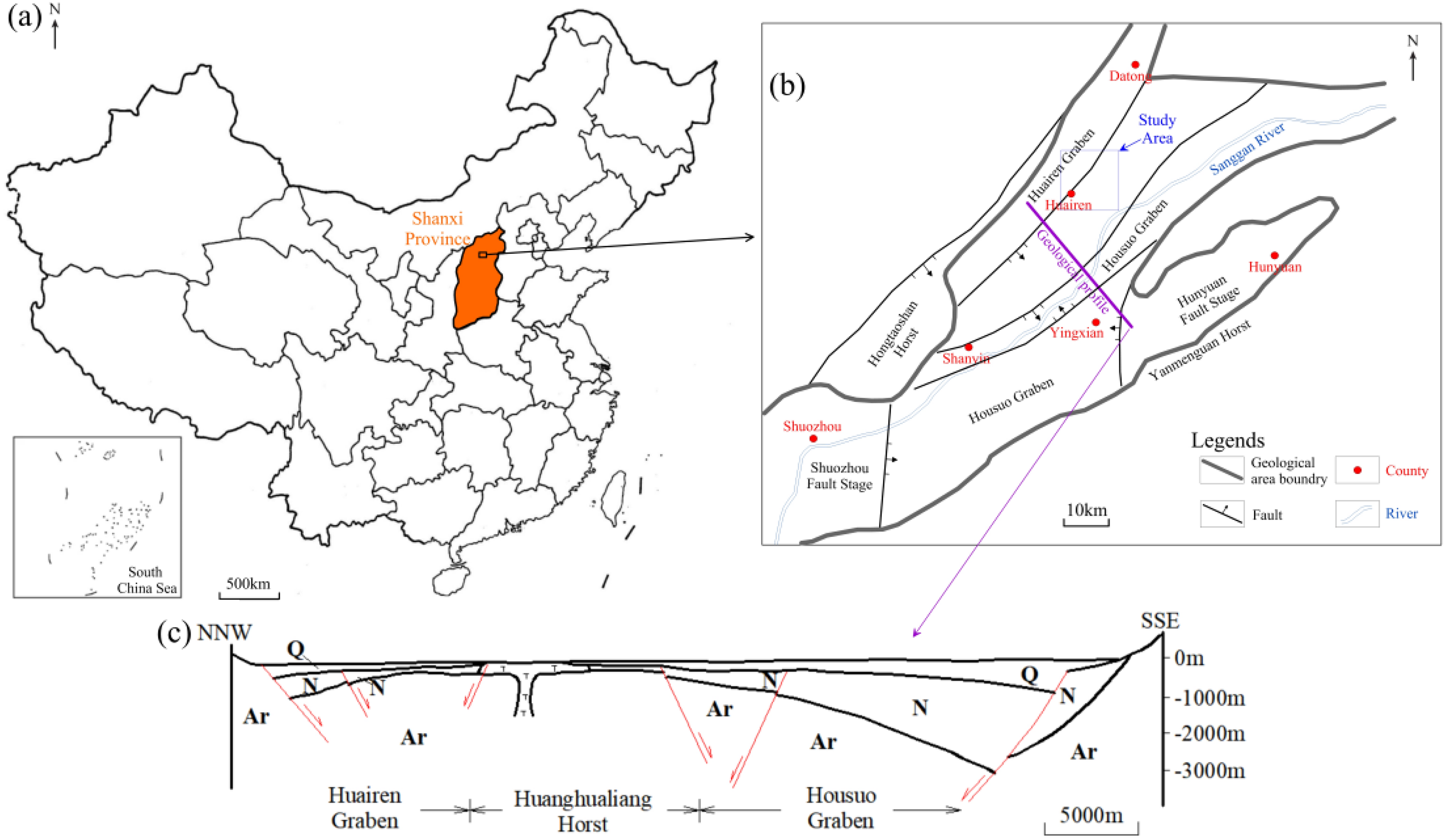
Geological structure map of the Sanggan River New Rift: (a) location of New Rift of Sanggan River Area; (b) schematic map of geological structure; (c) geological profile of the Sanggan River New Rift (cited from Xie et al., 2013).

Geophysical features of the study area

Different conductivities are found during the formation of different rocks. After long-term metamorphism, the formation of most rocks is complete and compact, without any fracture. In the horizontal direction, the resistivities remain constant, then increase gradually with increasing depth in the vertical direction.

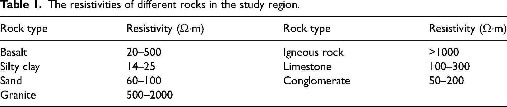
After receiving the intermittent leakage replenishment of surface water and vertical infiltration replenishment of atmospheric precipitation, the pore water of the overlying loose layer can flow into the deep igneous rock basement via the rock fissures and fault fracture zone. An aquifer is an underground layer of water stored in the igneous rocks. The resistivities of eruptive igneous rocks (e.g. rhyolite, basalt, etc.) are relatively lower (20–500 Ω·m) than granite (>500 Ω·m), while higher than the sediments of surrounding rocks. Hence, the differences in resistivities between sedimentary surrounding rocks and igneous rocks are determined using the geophysical method for identifying igneous rock locations and then exploring geothermal resources (Zhang et al., 2016) (Table 1).

Furthermore, the resistivities can alter in regions with the presence of faults. The fault activity can induce a fracture zone surrounding the faults, leading to a hydraulic relation between the lower and upper strata. In such manner, an anomaly region with low-resistivity is generated near the faults, which appears steeper on the resistivity profile. This may reflect the occurrence of faults, after which the location of geothermal resources can be identified.

Method of numerical simulation

Based on the close relationship of the key elemental resistivity of the geothermal system, and there is much interconnected pore water with strong conductivity in the low-resistivity faults, a simplified geothermal system resistivity model is developed, to simulate the geological conditions of the study area.

Generally, the basic structure of thermal reservoir is deep bedrock. Compared with the shallow stratum, the resistivity of the deep bedrock as the thermal reservoir is relatively high, which is the main target of electromagnetic exploration. In addition, the migration channel of geothermal fluid is the fault within the geothermal system. To meet the space demand of fluid migration, the fault is large in scale and has good water abundance, which makes the fault have good water and thermal conductivity. Due to the strong water-rich property of the fault, compared with the surrounding rocks, the fault is usually reflected as low resistivity, and is also the geophysical target of geothermal exploration (Bastani et al., 2011; Cairns et al., 1996). As demonstrated in Figure 2(a), the basic model contains four layers with deep and shallow resistivities of 100, 200, 500 and 1000 Ω·m. Given that strata dislocation may be induced by faults, the resistivities of all layers are staggering along the faults (Figure 2(b)). The design of this model aims to focus on the low-resistivity feature of the water-conducting faults. Hence, the faults are placed in the high-resistivity layered surrounding rocks.

Figure 2.

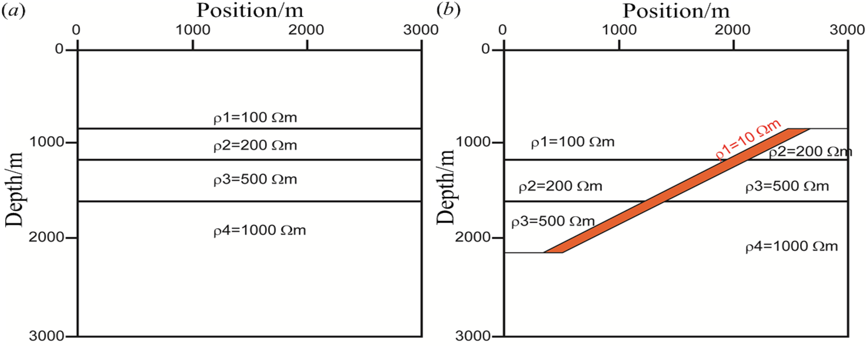
Simplified geothermal system resistivity model the faults as a target body: (a) is a background model, while (b) involves fault dislocation.

By CSAMT and TEM numerical simulations, the anomalous responses of the two methods to faults were compared, and the abilities of the two methods to identify and characterize faults were analyzed, which verified the complementarity of the two methods in detecting faults with different characteristics.

Regarding to the numerical simulation methods, many scholars have done a lot of researches, and the commonly used methods are as follow: finite volume method, finite difference method, finite element method, and integral equation method, etc. In this paper, an open-source code SIMPEG is used as the numerical simulation program, and finite volume method is used as the forward method, as displayed in the “Appendix” part.

Assumption of CSAMT responses

According to the simplified geothermal system resistivity model, the abnormal responses of CSAMT with various fault characteristics (resistivity, dip angle and width) are subjected to numerical simulation and analysis. The transmitting current and transmitting source length are normalized during the estimation of apparent resistivity.

CSAMT responses to the faults with various resistivity values

In the simplified geothermal system resistivity model, the fault's resistivity is 10 Ω·m. In the half-space strata, the faults can be considered as a plate-like, angularly inclined body with a downward extension. A massive amount of cracks is found in the fault region, which are filled by breccias and different resistivities of the filled substances, which can determine the features of the fault resistivity. Hence, the resistivity of faults often alters within a broad range. Then, fault models with various resistivities (10, 50 and 100 Ω·m), fault dip angle of 30° and width of 70 m are developed, and forward simulations are conducted to determine all responses. Later, their apparent resistivity are measured (Figure 3(a)–(c)).

Figure 3.

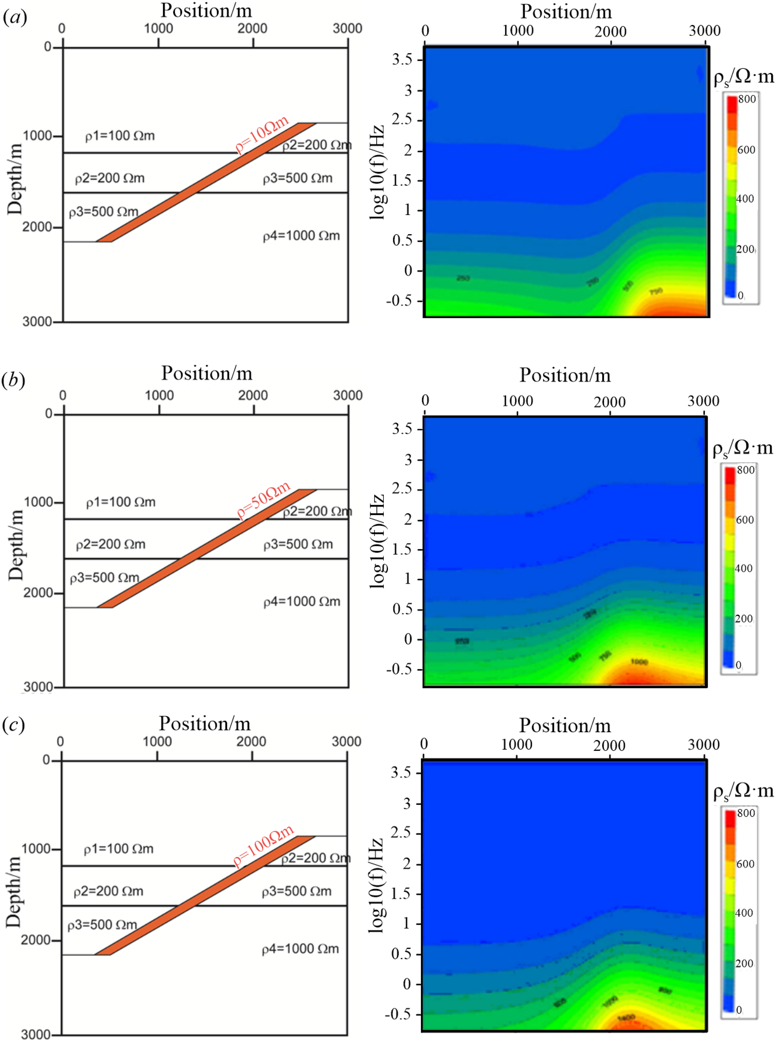
The models where the fault resistivities are 10, 50 and 100 Ω·m, together with the apparent resistivity. The apparent resistivity contour surrounding the faults is quite smooth when the fault resistivities are low (10 and 50 Ω·m), in which the apparent resistivity contour changes relatively more gently compared with (c). With increasing fault resistivities, the apparent resistivity contour increases greatly. Overall, the differences in fault resistivities can reflect a distinct apparent resistivity profile.

CSAMT responses to the faults with various dip angles

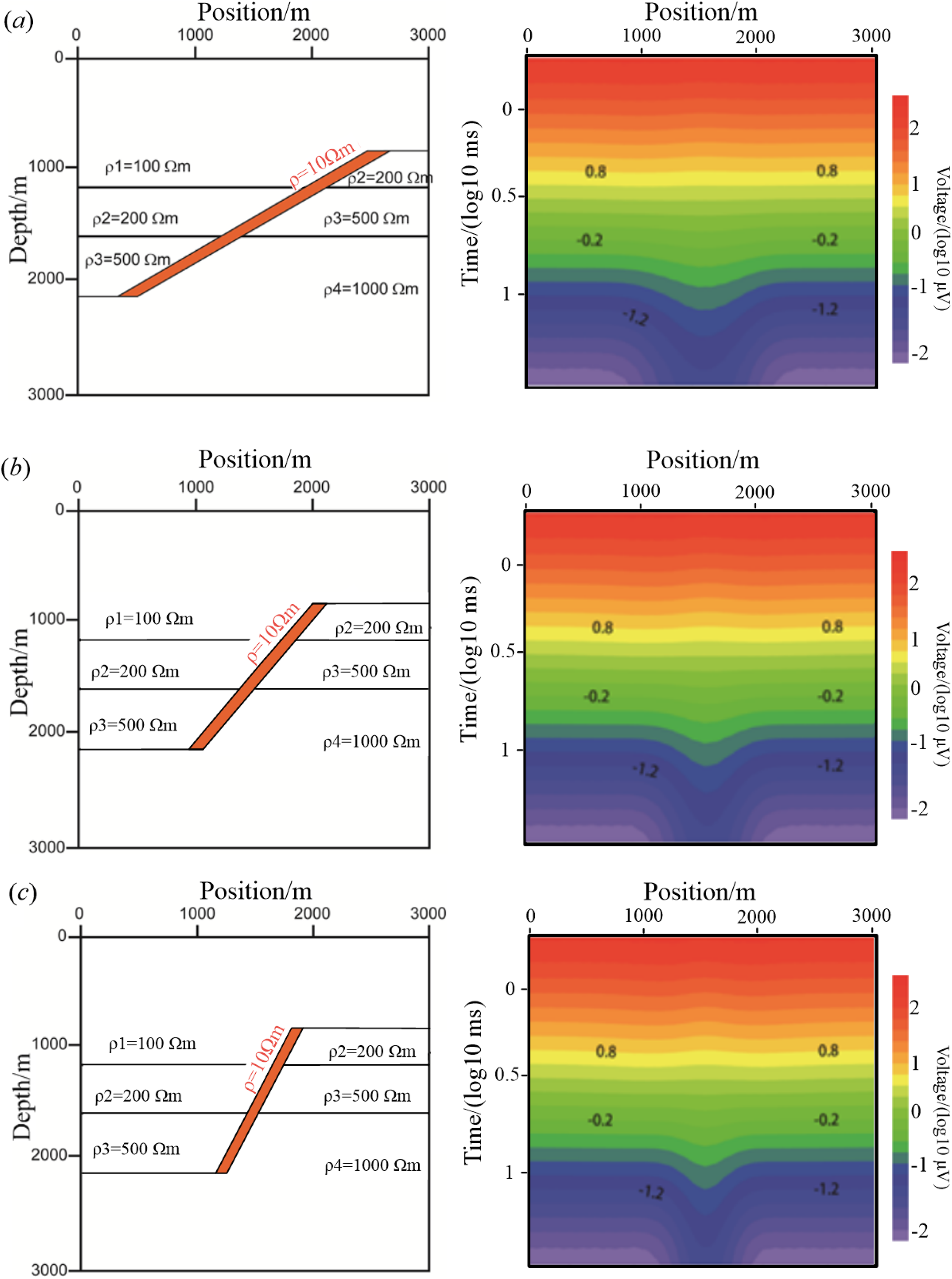
The dip angle of the faults is a crucial indicator of geothermal exploration. Therefore, fault models with various dip angles (dip angles: 30°, 45° and 60°, width: 70 m, fault resistivity: 10 Ω·m) are developed and forward simulation is conducted (Figure 4(a)–(c)).

Figure 4.

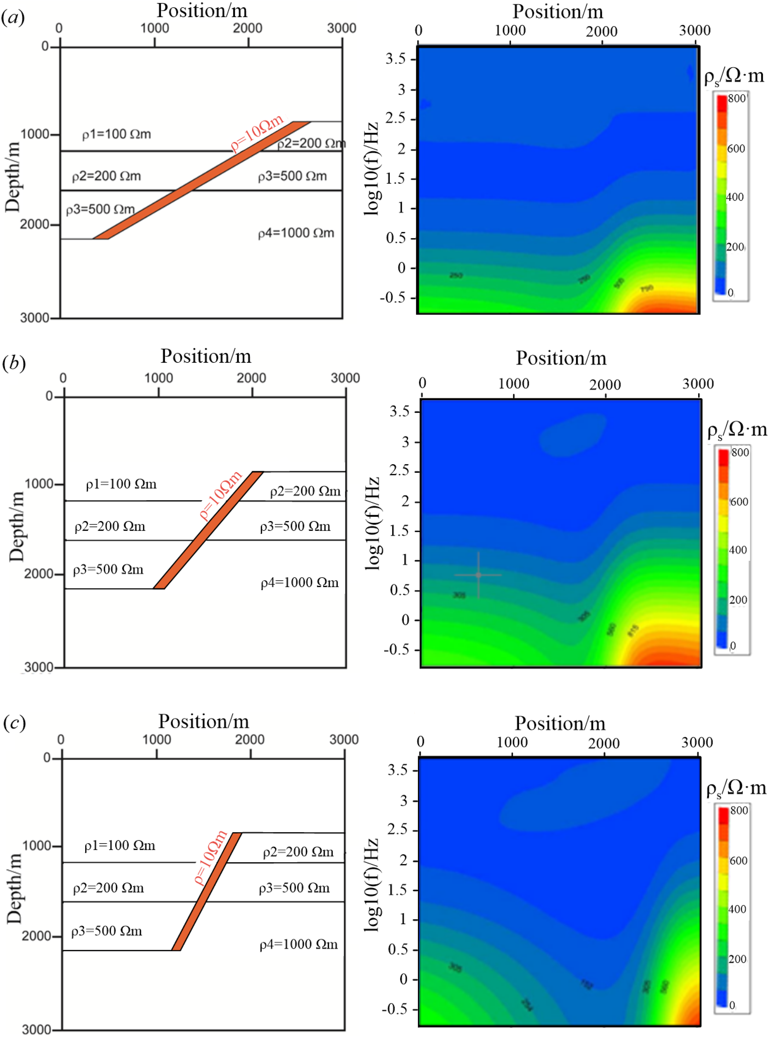
The models with fault dip angles of 30°, 45° and 60°, together with apparent resistivity profile. The “sags” is observed in the fault position of the apparent resistivity profile when the dip angles are 30°, 45° and 60°. The larger the dip angles, the higher the degrees of “sag”. The dip exceeds the actual fault.

CSAMT responses to the faults with various widths

Width can be used to determine the size of faults. Then, the widths of faults are 30, 70 and 100 m, dip angle is 30° and fault resistivity is 10 Ω·m, and forward simulation is conducted (Figure 5(a)–(c)).

Figure 5.

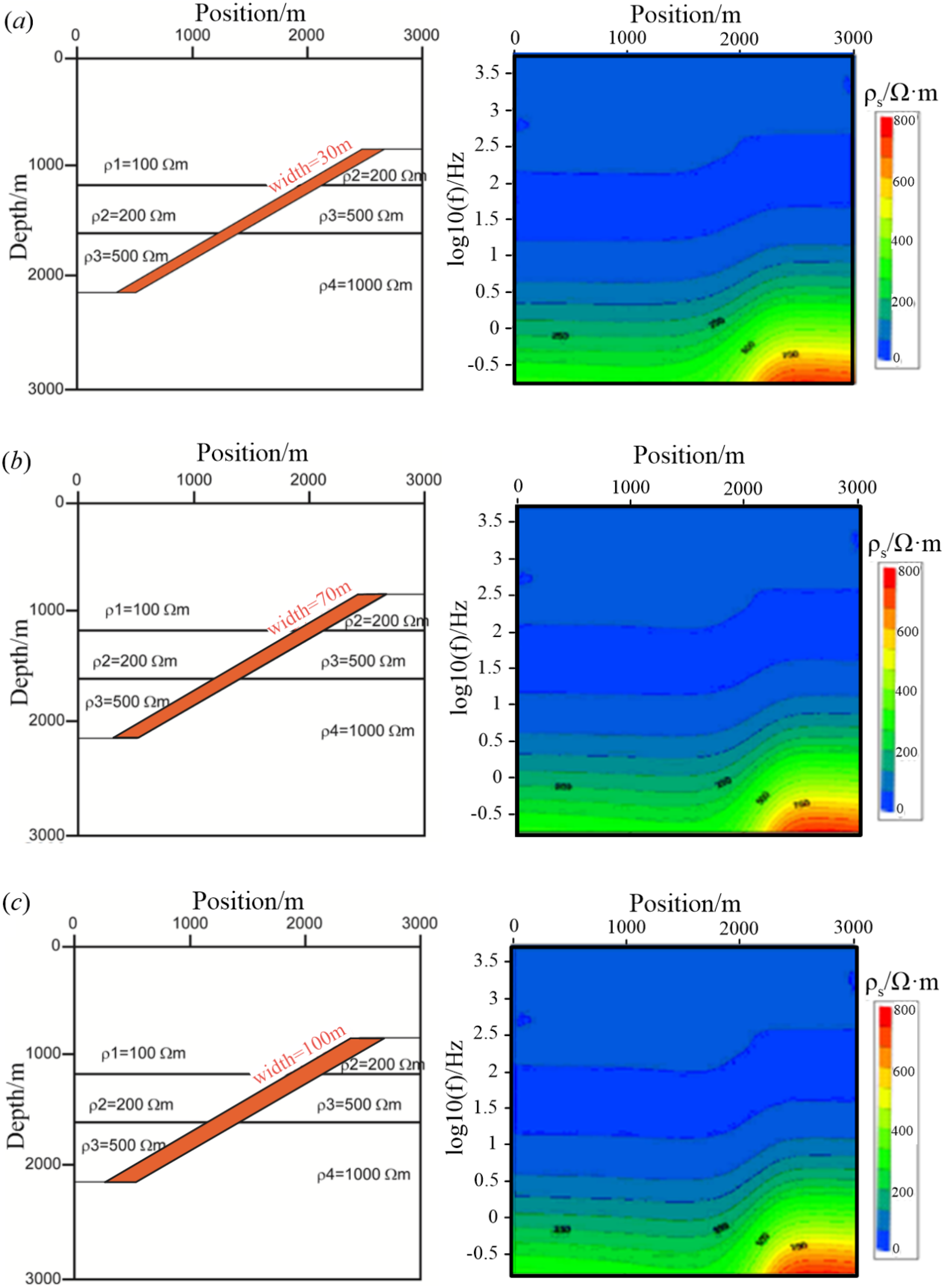
The widths of faults are 30, 70 and 100 m, together with the apparent resistivity profile. The “sags” is observed around the point 1500 when the widths are varied. Then, the apparent resistivity increases, which agrees well with the actual shape of the faults in resistivity model shown on the left side. With increasing fault widths, the degree of “sags” in the apparent resistivity contour slightly elevates. Therefore, it remains hard to precisely measure the actual fault width according to the features of apparent resistivity contour.

Assumption of TEM responses

According to the stimulation of low-resistivity fault models with various characteristics (resistivity, dip angle and width), the capability of CSAMT to determine low-resistivity faults was evaluated. Given that the apparent resistivity of TEM can be classified as late and early time channels, it remains hard to include all time channels into the apparent resistivity calculation formula. Hence, TEM analysis is conducted with voltage response (μV) at various moments.

The following parameters are used for TEM numerical calculation: the voltage response s at various moments are received in the center of the receiving loop; the transmitting source is a single-turn square loop (1000 × 1000 m); three receiving points are set in each receiving loop, the distance between the receiving points is 100 m, and the center of the transmitting loop coincides with the second receiving point; the transmitting loop moves along the direction of the surveying line, and the distance of each movement is 300 m; the number of time channels is 22; the time range is 0.48–28.7 ms; the transmitting waveform is a bipolar rectangular pulse (Figure 6). The geoelectric model is similar to that described in previous section.

Figure 6.

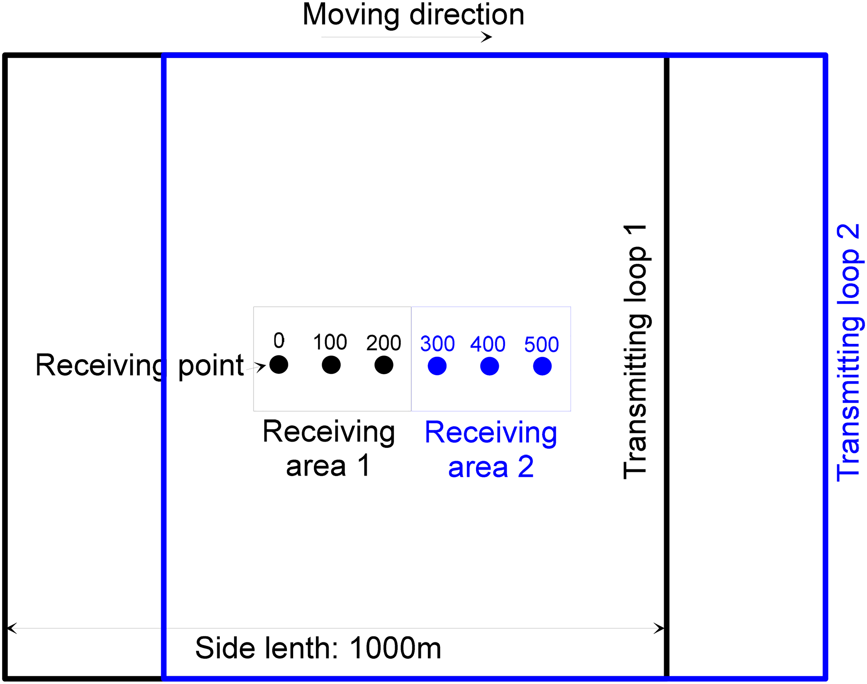
Schematic diagram of the TEM transmitting device.

TEM responses of the faults with various resistivities

The simplified models with various resistivities of 10, 50 and 100 Ω·m, width of 70 m, and dip angle of 30° are developed, and the VRs are measured. Considering the large buried depth, the anomaly response appears primarily in the late time channels of the TEM response, whereas the early time stages are not significantly influenced (Figure 7(a)–(c)).

Figure 7.

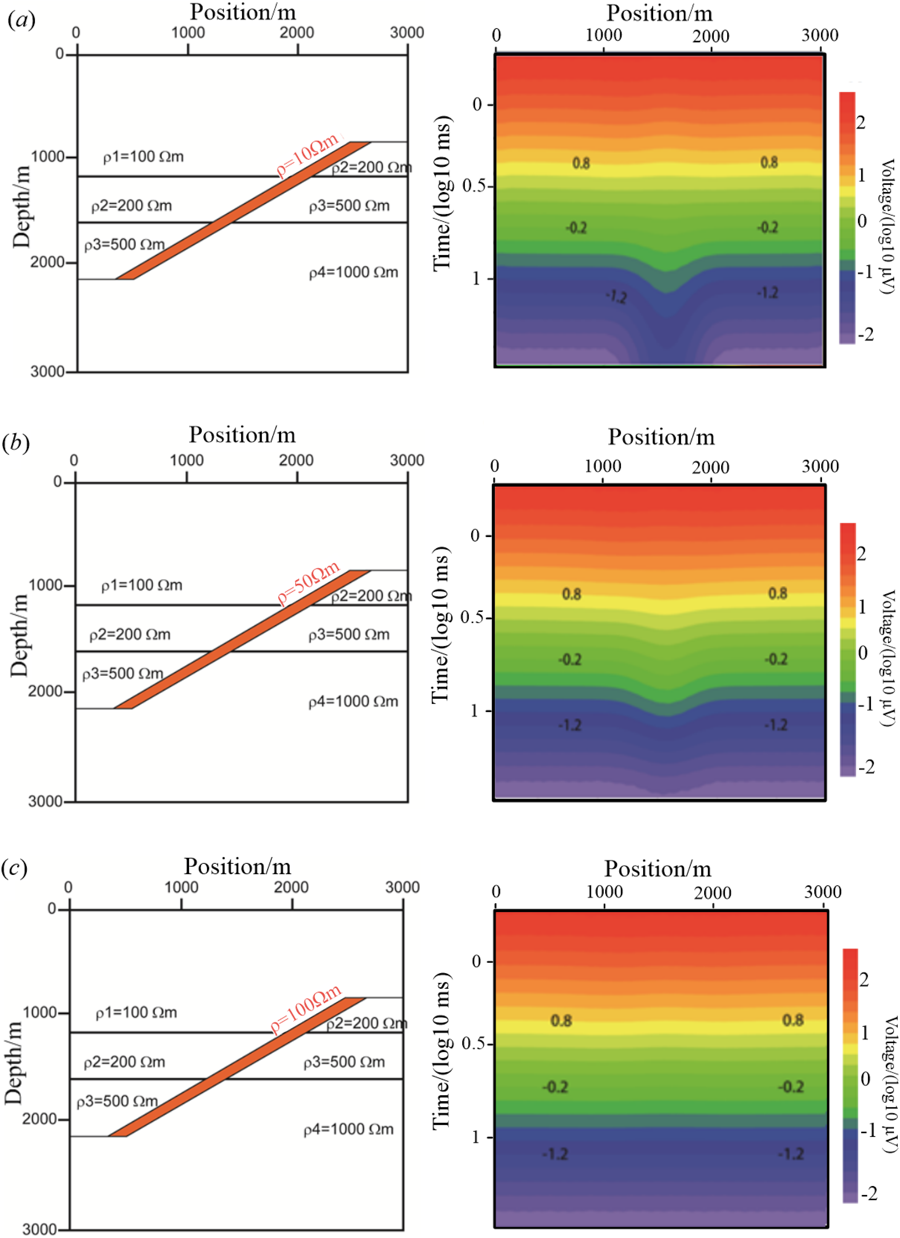
The models with fault resistivities of 10, 50 and 100 Ω·m, together with VR profile. A significant anomaly is observed when the fault resistivity is low, with its maximum value is located at the midpoint of the faults. The smaller the resistivity, the more significant the abnormal VR. No large anomaly is formed in the VR profile, and the difference in resistivity between the faults and surrounding rocks is small, when the fault resistivity is 100 Ω·m. This indicates that TEM is not easy to identify the faults if the difference is small.

TEM responses to the faults with various dip angles

Simplified models with various dip angles of 30°, 45° and 60°, resistivity of 10 Ω·m and width of 70 m, are developed, and the VRs are measured (Figure 8(a)–(c)).

Figure 8.

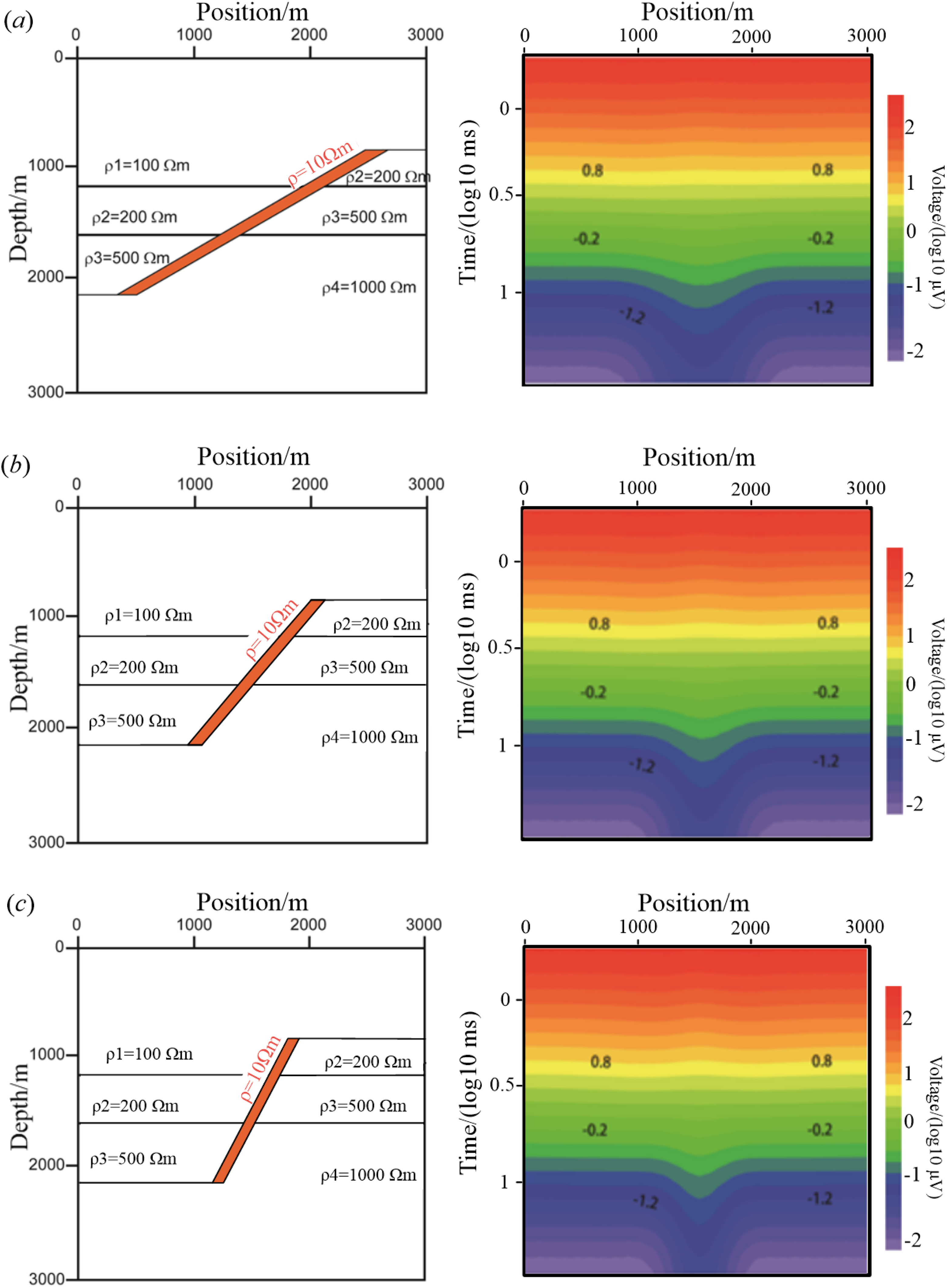
The models with various dip angles of 30°, 45° and 60°, together with the VR profile. The VR is altered when the dip angle changes. With increasing dip angles, the surveying point that receives abnormal VR decreases gradually, while the abnormal VR amplitude increases gradually, indicating that TEM is responsive to the fault dip angles.

TEM responses to the faults with various widths

Simplified models with various widths of 30, 70 and 100 m, dip angle of 30° and resistivity of 10 Ω·m are developed, and the VRs are measured (Figure 9(a)–(c)).

Figure 9.

The models with various widths of 30, 70 and 100 m, together with the VR profile. The VR changes when the width is altered. With increasing fault widths, the abnormal VR amplitude becomes more apparent, indicating that TEM is responsive to the fault width.

Results of numerical simulation

Using the numerical simulation based on the abnormal changes in the resistivities, dip angles and widths of the low-resistivity faults in the simplified geothermal system model, both TEM and CSAMT are conducted, which can be inferred as follows.

The impact of low-resistivity faults on CSAMT responses occurs primarily in the low-frequency band, while that on TEM responses is more towards the late time channels. Data still can be obtained with relatively high quality in the low-frequency band, while the quality of the late TEM responses is normally lower, and the fault resolution of CSAMT is higher than that of TEM.

Meanwhile, the abnormal responses caused by the fault width can be clearly distinguished by TEM responses but not CSAMT responses, showing that TEM has an outstanding capability to explain the characteristics of low-resistivity fault compared with CSAMT. Additionally, the faults are mostly characterized by the resistivity of dislocation on the apparent resistivity profiles of CSAMT, and the lower and upper plates of faults can also be distinguished by CSAMT.

Although low-resistivity faults can be identified by the two methods in this model, these methods show an in-depth exploration of complementary and capability for detailed description, which are applicable to geothermal exploration.

Example of field experiment

As shown in Figure 10, a surveying line was arranged in the study area.

Figure 10.

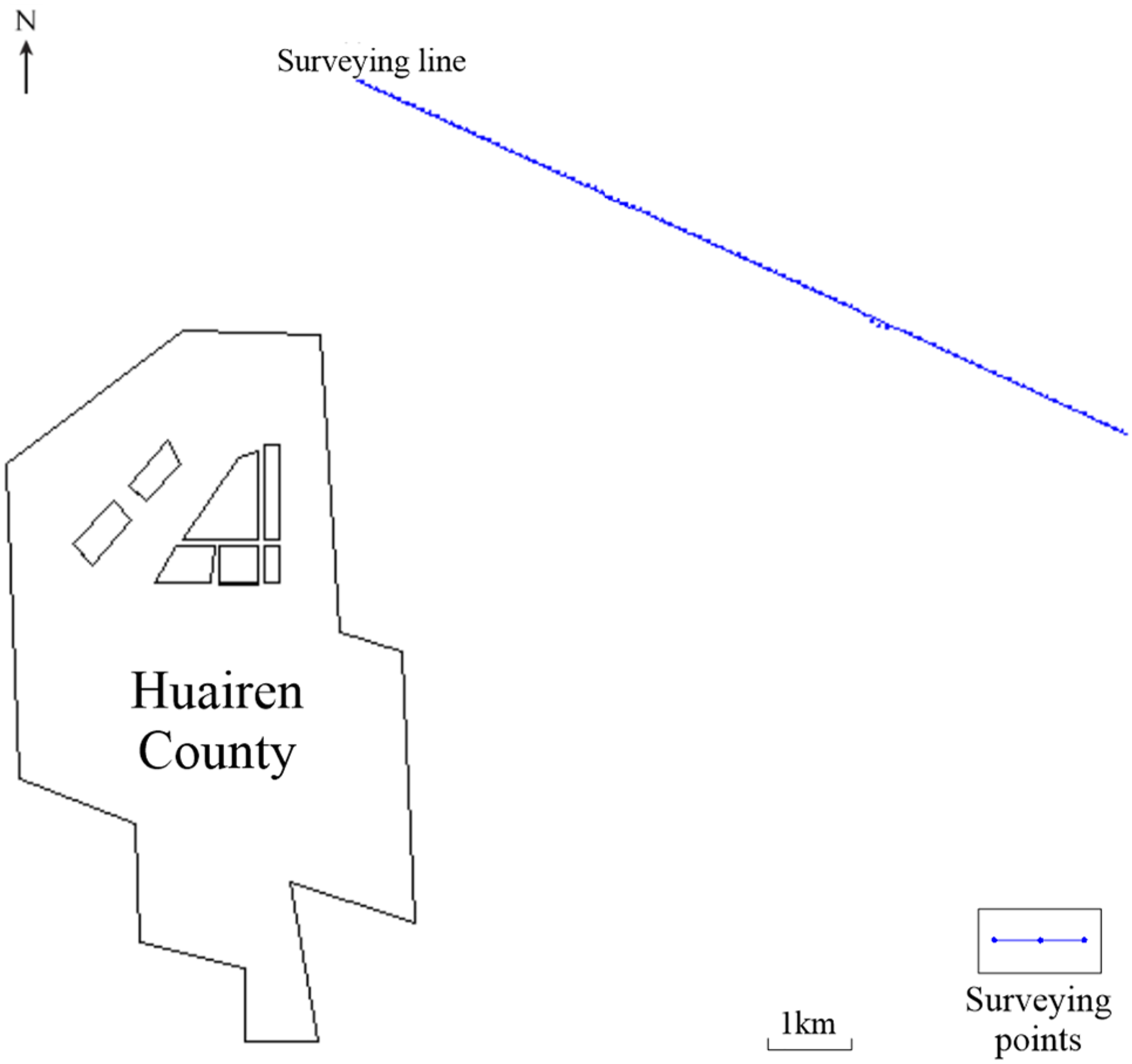
Layout of the project.

The GDP32II multifunctional electrical method workstation was used for the exploration of CSAMT. The transmitting-receiving distance, current and pole distance AB are 6 km, 14–16 A and 1500 m, respectively; the signal frequency range is 0.125–7680 Hz; the distance between the surveying points is 100 m for lines 10 and 60 and 50 m for lines 59 and 64. The same instrument was also used for TEM exploration, along with the center loop device. The transmitting current, frequency and source are 15 A, 16 Hz and a 1000 × 1000 m single-turn loop, respectively; the distance between the surveying points is 50 m. After completing the CSAMT survey, line 60 is set as the TEM surveying line, due to an obvious resistivity anomaly of CSAMT, and a comparison between the two methods is made.

Verified situation

To process the obtained data, the GDP32II data preprocessing software is applied for data sorting and removal of dead pixels. Then, TEM-1D software (Guo et al., 2020; Sudha et al., 2014) and CSAMT-2D software (Fu et al., 2013; Hedlin et al., 1990; Kouadio et al., 2020) of Zonge Co. were used to invert the data. The two softwares use the OCCAM inversion method (Constable and Parker, 1987; Xing et al., 2021) to solve the Green function and the adjoint function in the 2D domain and the 1D domain, respectively, to obtain the Jacobian matrix required for the inversion, and then realize the spatial inversion of the electric field data.

The inversion data of TEM and CSAMT resistivity profiles are displayed in Figure 11(a)–(c).

Figure 11.

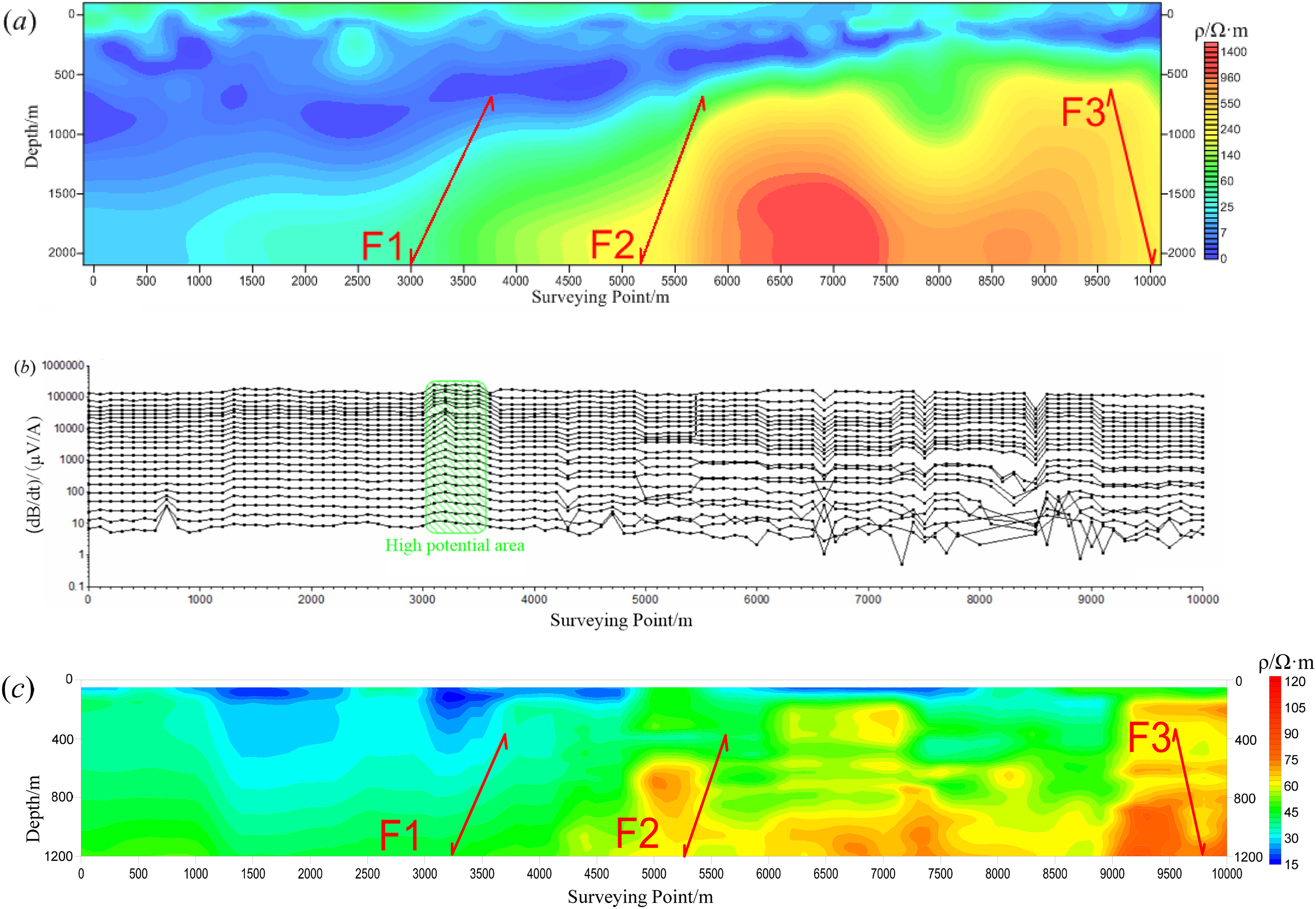
(a) Resistivity profile of CSAMT surveying line. (b) Secondary field potential profile of TEM surveying line. (c) Resistivity profile of TEM surveying line.

The CSAMT inversion results are shown in Figure 11(a). It can be seen that the resistivity from shallow to deep is low–medium–high and has a significant three-layer structure. The specific analysis of each layer is as follows.

The first electrical layer: the low resistivity layer, the shallow layer in the profile, the inversion resistivity is basically continuous along the profile, and the thickness ranges from 15 to 100 m; it is speculated that this layer is a dry argillaceous sand and clay layer of the quaternary, and the relatively thick part is the part where the stratification of the tertiary and quaternary is not significant. The second electrical layer: the medium resistivity layer, the resistivity basically spreads along the section, the continuity of the local area is poor, the depth range is between 200 and 750 m, and the thickness increases from right to left; it is speculated that this layer is the loose accumulation of the Pliocene of the Late Tertiary. The third electrical layer: a relatively high resistivity layer, the top interface buried depth is between 300 and 750 m; it is speculated that this layer is the basement of basalt or middle-deep metamorphic rock of Wutai Group. The electrical resistivity distortion occurred in the vicinity of the 3500 point, the 5600 point and the 9750 point in the electrical layer, and it is inferred that these places are fault locations.

The TEM inversion results are shown in Figure 11(b) and (c). It can be seen that the TEM profile features are similar to those of CSAMT, the electrical layers are basically distributed in layers, and the resistivity from shallow to deep also shows a low–medium–high three-layer structure. The inferences for each layer are described as follows.

The resistivity of the shallow strata is relatively small, and it is inferred that the quaternary sand and clay layers are in the range of 15 to 200 m in thickness. There is no significant stratification between the quaternary and the tertiary in this layer. The resistivity in the middle part increases, and the depth decreases from left to right, which is inferred to be loose deposits of the Late Tertiary Pliocene. The resistivity of the deep part is relatively high, and the depth on the right side is small, and the top interface is buried at a depth of 300 m, which is presumed to be a basalt or a mid-deep metamorphic rock base in the Wutai Group. In the 3000–3500 section, the resistivity is distorted, showing the characteristics of low resistivity, and it is inferred that this section is the fault F1 part; in the 3000–3500 section of 11 (b), the secondary field potential has a high value anomaly, which is consistent with the low-resistance feature in the resistivity cross-sectional diagram, and is also the electrical feature exhibited by the fault F1; Section 7500–8800 has a high resistance area in the deep, which is inferred as the location of basalt.

According to the results of the inverted resistivity, the geological profile of the surveying line was drawn, as shown in Figure 12.

Figure 12.

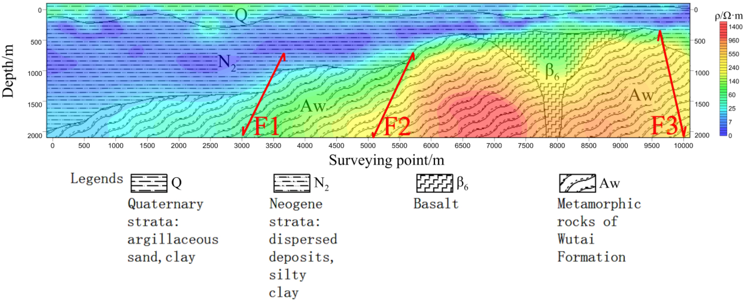
Geological profile of the surveying line.

Discussion

In general, the resistivity profiles of TEM and CSAMT are relatively similar, indicating a layered distribution of low-to-high resistivity from shallow to deep formation. The depth of high-resistivity region gradually reduces with increasing number of the surveying lines. A deep high-resistivity component can be obviously found starting from point 6000. The positions of F1, F2 and F3 faults in the resistivity profile can be revealed by the two methods, which indicate an excellent effect with regard to mutual verification.

Meanwhile, some differences are found in the geothermal exploration results of the same surveying line between the two methods. Based on these differences, the advantage, disadvantage and complementarity of the two methods in actual exploration are presented as follows: (1)

The geothermal exploration of TEM is greater than CSAMT in the shallow layer:

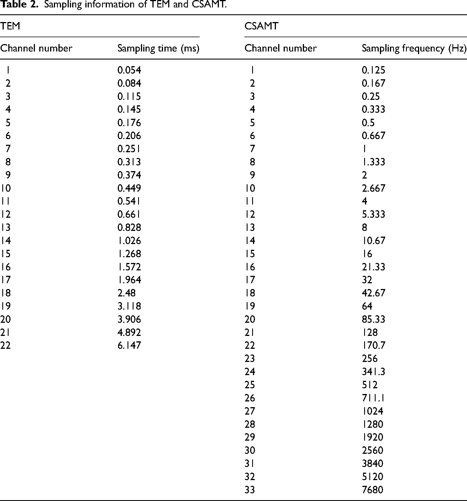
The signals of TEM and CSAMT have similar signal: noise ratios for determining shallow formation. However, the sampling density and channel number of TEM are relatively larger than CSAMT during shallow formation (Table 2). In view of resistivity profile, the resistivity of TEM in shallow formation is relatively constant in the horizontal direction, which reflects the actual geological features. Meanwhile, the positions of the fault shallow part examined by TEM is much obvious, thus providing more solid evidence to reveal the extension positions of the faults in the shallow and middle parts.

(2)

The exploration of CSAMT is greater than on TEM for deep high-resistivity strata:

Table 1.

The resistivities of different rocks in the study region.

Rock type	Resistivity (Ω·m)	Rock type	Resistivity (Ω·m)
Basalt	20–500	Igneous rock	>1000
Silty clay	14–25	Limestone	100–300
Sand	60–100	Conglomerate	50–200
Granite	500–2000

Table 2.

Sampling information of TEM and CSAMT.

TEM		CSAMT
Channel number	Sampling time (ms)	Channel number	Sampling frequency (Hz)
1	0.054	1	0.125
2	0.084	2	0.167
3	0.115	3	0.25
4	0.145	4	0.333
5	0.176	5	0.5
6	0.206	6	0.667
7	0.251	7	1
8	0.313	8	1.333
9	0.374	9	2
10	0.449	10	2.667
11	0.541	11	4
12	0.661	12	5.333
13	0.828	13	8
14	1.026	14	10.67
15	1.268	15	16
16	1.572	16	21.33
17	1.964	17	32
18	2.48	18	42.67
19	3.118	19	64
20	3.906	20	85.33
21	4.892	21	128
22	6.147	22	170.7
		23	256
		24	341.3
		25	512
		26	711.1
		27	1024
		28	1280
		29	1920
		30	2560
		31	3840
		32	5120
		33	7680

Given that the time interval is large among different sampling channels of TEM in the late time channels, the exploration depth is markedly limited, the late signal error is high, and the signal:noise ratio is low, the geothermal exploration effect of deep electrical structures is reduced. In CSAMT exploration, the lower the signal frequency is, the greater the detection depth will be. CSAMT has stronger penetrating ability and higher energy at lower frequencies, but satisfactory exploration results can still be obtained in the deep part. According to the apparent resistivity profile, the reflection of deep basement strata is weak and the deep structure of TEM is not clear, while CSAMT obviously exhibits the morphology of deep basement structure. (3)

The exploration of TEM is greater than CSAMT for water-conducting faults:

The pure anomaly field of TEM is responsive to low-resistivity targets, as revealed by the exploration of F1 faults. There is clear discontinuity observed for the apparent resistivity profile of TEM in the low-resistivity region, while CSAMT shows nearly no reflection on the F1 fault. This is supported by the secondary field potential of TEM, in which a high anomaly is observed in the secondary field potential near the fault F1. The primary benefit of CSAMT for determining faults is that it can differentiate the lower and upper plates of the faults.

After completing the geothermal exploration, the verification of drilling was conducted at point 3350. The drills encountered underground heat at 1610 m, and then a pumping test was performed. Based on the finding geothermal system of the pumping test, the unit output of underground heat was 233 m³/d, and the temperature of hot water was 58°C. These data indicated the existence of geothermal water in the faults and igneous rocks.

Conclusion

Through numerical simulation and anomaly comparison, it is found that both methods show different abilities to describe the fault details. Moreover, the resolution of CSAMT is stronger for deep target, similar to the capability of TEM for describing the details of shallow target. These two methods can identify targets at various depths. Moreover, the two methods are obviously complementary, and they are applicable for geothermal exploration. The actual exploration results of TEM and CSAMT on the same surveying line demonstrate that CSAMT outperforms TEM for the deep basement exploration of magmatic rocks, whereas TEM outperforms CSAMT for the exploration of shallow target and water-conducting fault structure. The comprehensive electromagnetic method used in this study can enhance the integrative effect of two complementary methods and overcome the limitation of a single method.

For exploring geothermal resources in Huairen County, the geological results are obtained as follows. It can be inferred that F1, F2 and F3 faults are identified, and the main channel for underground hot water is F1. The mid-deep metamorphic rock or deep basalt basement may involve a GR storage structure. Our findings in geothermal system highlight the advantages and disadvantages of TEM and CSAMT with regard to geothermal exploration.

Footnotes

Acknowledgements

This research is supported by the Comprehensive Investigation and Evaluation Project of Geothermal Resources in the Cuona-Chayu Area, Tibet (No. DD20211548).

Data availability statement

The data which support the findings of this study are available from the corresponding author upon request.

Declaration of conflicting interests

The author(s) declared no potential conflicts of interest with respect to the research, authorship, and/or publication of this article.

Funding

The author(s) received no financial support for the research, authorship, and/or publication of this article.

ORCID iD

Jie Zhu

Appendix

References

Bai

Liao

Zhao

, et al. (1994) Inferring the magma heat source of the Tengchong Rehai hot field from the MT detection results. Chinese Science Bulletin 4: 17.

Bastani

Savvaidis

Pedersen

(2011) CSAMT measurements in the frequency range of 1250 kHz to map a normal fault in the Volvi Basin, Greece. Journal of Applied Geophysics 75(2): 180–195.

Cairns

Evans

Edwards

(1996) A time-domain electromagnetic survey of the TAG hydrothermal mound. Geophysical Research Letters 23(23): 3455–3458.

Chen

Liu

, et al. (2011) Application of integrated geophysical techniques in investigation of urban active faults: Take Úrümqi Bagangeothermal systemhihua fracture as an example. Progress in Geophysics 34(4): 1584–1591. (in Chinese with English abstract).

Constable

Parker

(1987) Occam’s inversion: A practical algorithm for generating smooth models from electromagnetic sounding data. Geophysics 52: 289–300.

Wang

Shi

, et al. (2008) Applications of CSAMT for deep geothermal exploration in high level ambient noises areas in Beijing. Journal of Engineering Geology 15(Suppl.): 203–207 (in Chinese with English abstract).

Didana

Thiel

Heinson

(2014) Magnetotelluric imaging of upper crustal partial melt at Tendaho graben in Afar, Ethiopia. Geophysical Research Letters 41(9): 3089–3095.

(2013) Application of the CSAMT method to groundwater exploration in a metropolitan environment. Geophysics 78: B201–B209.

Huang

Liu

, et al. (2019) Multi-electrode resistivity method and CSAMT method in geothermal exploration of Babei area in Huichang County, Jiangxi Province. Geology in China 46(04): 927–936.

10.

Guo

Liu

Zheng

(2020) Analytical algorithms of Jacobian matrix in one-dimensional Occam inversion of central loop transient electromagnetism based on all-time apparent resistivity. Geophysical and Geochemical Exploration 44(3): 559–567.

11.

Hedlin

Constable

(1990) Occam inversion to generate smooth, two-dimensional model from magnetotelluric data. Geophysics 55(12)(Decomprehensive electromagnetic methodber. 1990): 1613–1624.

12.

Heise

Caldwell

Bannister

, et al. (2017) Mapping subduction interface coupling using magnetotellurics: Hikurangi margin, New Zealand. Geophysical Research Letters 44(18): 9261–9266.

13.

Heise

Ogawa

Bertrand

, et al. (2019) Electrical resistivity imaging of the inter-plate coupling transition at the Hikurangi subduction margin, New Zealand. Earth and Planetary Science Letters 524: 115710.

14.

Wang

(2011) Heat flow in the continental area of China: A new data set. Earth and Planetary Science Letters 179(2): 407–419.

15.

Kouadio

Liu

, et al. (2020) Two-dimensional inversion of CSAMT data and three-dimensional geological mapping for groundwater exploration in Tongkeng Area, Hunan Province, China. Journal of Applied Geophysics 83: 104204.

16.

Muñoz

(2014) Exploring for geothermal resources with electromagnetic methods. Surveys in Geophysics 35(1): 101–122.

17.

Muraoka

Uchida

Sasada

, et al. (1998) Deep geothermal resources survey program: Igneous, metamorphic and hydrothermal processes in a well encountering 500 C at 3729 m depth, Kakkonda, Japan. Geothermics 27(5–6): 507–534.

18.

Ozdemir

Arabaci

Palabiyik

(2021) Reevaluation of geothermal potential of ubukluda Graben (Western Anatolia, Turkey). International Journal of Earth Sciences Knowledge and Applications 3(2): 70–88.

19.

Ozdemir

Palabiyik

(2019) A new method for geological interpretation of 3D MT (magnetotelluric) depth maps of high-temperature and deep geothermal fields: A case study from Western Turkey. 2. International Congress of Applied Sciences, 28–30 October 2019, Ankara, Turkey, 28–42.

20.

Ren

Yin

Liu

(2017) Efficient modeling of time-domain AEM using finite-volume method. JEEG 22(3): 267–278.

21.

Robertson

Thiel

Meqbel

(2020) Quality over quantity: On workflow and model space exploration of 3D inversion of MT data. Earth, Planets and Space 72(1): 1–22.

22.

Singh

Maurya

Singh

(2018) Audio-manetotelluric investigation of sulfide mineralization in proterozoic-archean greenstone belts of Eastern Indian Craton. Journal of Earth System Science 127(3): 34.

23.

Smith

(2014) Electromagnetic induction methods in mining geophysics from 2008 to 2012. Surveys in Geophysics 35(1): 123–156.

24.

Spichak

Manzella

(2009) Electromagnetic sounding of geothermal zones. Journal of Applied Geophysics 68(4): 459–478.

25.

Sudha

Tezkan

Siemon (2014) Appraisal of a new 1D weighted joint inversion of ground based and helicopter-borne electromagnetic data. Geophysical Prospecting 62(3): 597–614.

26.

Tauber

Banks

Ritter

(2018) A high-resolution survey of the lapetus suture zone in South-west Scotland. Geophysical Journal International 153(3): 548–568.

27.

Tripathi

Shalivahan

Bagea

(2019) Audio-magnetotelluric investigation of bakreswar geothermal province, Eastern Indiajj. Journal of Earth System Science 71: 1472–1483.

28.

Xie

, et al. (2013) The tectonic character and oil-bearing properties of sangganhe fault depression. Science & Technology Vision 17: 5–6 (in Chinese with English abstract).

29.

Xing

Yuan

(2021) One-dimensional Occam’s inversion for transient electromagnetic data excited by a loop source. Geophysical and Geochemical Exploration 45(05): 1320–1328.

30.

, et al. (2013) Microtremor survey method: A new geophysical method for dividing strata and detecting the buried fault structures. Acta Petrologica Sinica 29(5): 1841–1845.

31.

Yang

(2017) On deployment of high-temperature deep geothermal wells in typical areas with hot dry rock potential in China. Geology and Exploration 53(2): 355–360. (in Chinese with English abstract).

32.

Yang

Liu

Zhang

, et al. (2009) Applying comprehensive geophysical prospecting method in geothermal exploration in Tianjin area. Global Geology 28(3): 351–360 (in Chinese with English abstract).

33.

Yee

(1996) Numerical solution of initial boundary problem involving Maxwell’s equations in isotropic media. IEEE Transactions on Antennas and Propagation 14(3): 302–307.

34.

Yin

Jin

(2007) The application of the integrated geophysical and geochemical methods to the geothermal exploration in a certain area of Inner Mongolia. Geophysical & Geochemcal Expioration 31(4): 313–316.

35.

Younis

El-Qady

Abd

(2015) AMT and CSAMT methods for hydrocarbon exploration at Nile Delta, Egyptj. Arabian Journal of Geosciences 8(4): 1965–1975.

36.

Zhang

Shuai

Zhang

(2019) Geothermal power generation in China: Status and prospects. Energy Science & Engineering 7(5): 1428–1450.

37.

Zhang

Jin

Wang

, et al. (2016) Relationship between magma-thermal field and hydrocarbon accumulation. Progress in Geophysics 31(4): 1525–1541 (in Chinese with English abstract)

Exploration of geothermal resources using comprehensive electromagnetic method

Abstract

Keywords

Introduction

Geological settings of the study area

Description of the study area

Geophysical features of the study area

Method of numerical simulation

Assumption of CSAMT responses

CSAMT responses to the faults with various resistivity values

CSAMT responses to the faults with various dip angles

CSAMT responses to the faults with various widths

Assumption of TEM responses

TEM responses of the faults with various resistivities

TEM responses to the faults with various dip angles

TEM responses to the faults with various widths

Results of numerical simulation

Example of field experiment

Verified situation

Discussion

Conclusion

Footnotes

Acknowledgements

Data availability statement

Declaration of conflicting interests

Funding

ORCID iD

Appendix

References