Sage Journals: Discover world-class research

Abstract

Recently, power systems have faced the challenges of growing electricity demand, reducing fossil fuels, and exacerbating environmental pollution due to carbon emissions from fossil fuel-based power generation. Integrating low-carbon alternative energy, renewable energy sources (RES), is becoming very important for energy systems. Effective management of the integration of the production capacity of RES is as important as the production capacity of wind farms with the production capacity of fossil fuel power plants. This article analyzed 850,660 data recorded by a wind farm from March 01, 2020, 00:00:00 to December 31, t2020, 23:50:00 were analyzed. And by using machine learning and extra tree, light gradient boosting machine, gradient boosting regressor, decision tree, Ada Boost, and ridge algorithms, the production power of the wind farm was predicted. The best performance predicting the turbine production power was assigned to extra tree, and the worst performance was related to the Ridge algorithm.

Keywords

Renewable energy sources wind farms fossil fuels extra tree ridge

1. Introduction

Renewable energy sources (RES) are increasingly important in reducing the world's carbon footprint (Caglayan et al., 2019). Alternatives to conventional fossil fuels include wind energy (Wang et al., 2018; Dai et al., 2019). For instance, European countries have significantly increased the number of newly constructed offshore wind farms. Eighty percent of the world's freshly built offshore wind capacity was in E.U. countries as of 2017 (Caglayan et al., 2019).

Offshore wind farms benefit from having more wind sources, luxurious building locations, and higher wind production capacity than onshore wind farms (Wang et al., 2019). As a result, the wind turbine sector has experienced a steady shift from onshore to offshore wind turbines. Meanwhile, because of the unpredictable environment in which they operate and the failures of offshore wind turbines, there is a growing focus on improving the performance of offshore wind turbines. The goal is to reduce the cost of energy gathered from newly installed RES (Chen et al., 2018; Yin and Zhao, 2019) and enhance the efficiency of that energy (Castellani et al., 2017). Accurate power forecasting is difficult, but it is critical for wind turbines because it may lower operating costs (Wang et al., 2017), which is essential for wind farms transitioning from onshore to offshore (Arun Kumar et al., 2019).

Many scholars, such as Patak et al. (Pathak et al., 2021), Chudari et al. (Chaudhary et al., 2020), and Zumar et al. (Zameer et al., 2015) have designed software models for producing predicted power using RES and achieved acceptable results in predicting the production power of wind turbines. The development of appropriate software models for producing predicted power using RES is currently being investigated. These algorithms have failed to deliver acceptable results under various wind conditions.

In today's world, short-term memory prediction approaches and light gradient amplification machine models are popular (Duan, 2021; Singh et al., 2021). In RES, wind power is a significant player. In recent years, production capacity has increased exponentially (Manobel et al., 2018). Yang et al. (Yang et al., 2021) headed a team of academics who employed to create predictions, a fuzzy C-means (FCM) clustering algorithm was used. It has been established that the novel spatio-temporal correlation (STCM) model for wind energy prediction based on convolutional neural networks and long-term memory (CNN-LSTM) is more successful than standard models in extracting better spatial and temporal properties. A unique spatio-temporal (STCM) operation based on convolutional neural networks and long-term short-term memory (CNN-LSTM) has been created to predict wind energy, extracting better spatial, and temporal characteristics than previous models.

Power consumption has surged due to the industrial revolution, and fossil fuels have been exploited extensively, resulting in an impending energy crisis (Zhao et al., 2016). Regulative activities that stimulate the use of renewable energy are being encouraged across the globe to help alleviate the energy problem. Wind energy has lately received much attention as an RES. Wind energy has grown in popularity owing to its widespread availability, cheap investment cost (U.S. Department of Energy), and lack of carbon emissions. Wind energy aids in the reduction of pollution (Jong et al., 2016). It is being implemented all around the globe as a strategy to minimize greenhouse gas emissions. Additionally, substituting thermal energy with wind generating saves money on gasoline since the wind has no fuel expenditures. According to the Worldwide Wind Energy Council (Global Wind Energy Council), the total wind power capacity in the global market reached 486 GW in 2016. Wind power is predicted to grow dramatically, eventually leading to a zero-emission power system (Shafiee et al., 2016; Tomporowski et al., 2017). By 2030, the U.S. Department of Energy's Renewable Integration Target calls for wind to provide 20% of total energy (U.S. Department of Energy, 2008). Independent system operators (ISOs) generate considerable amounts of wind electricity and grow their wind output. Meteorological variables, particularly wind speed, significantly impact wind power. Because wind energy is so erratic and intermittent, the amount of electricity produced is uncertain. Operations of the electricity system, such as distribution, dispatching, peak load management, etc., are significantly impacted by this uncertainty (Athari and Wang, 2018). Since wind energy is regarded as one of the most promising RES, wind turbines are being built worldwide. In 2015, 12.8 GW of wind energy was installed annually in Europe, with offshore wind power making up more than 25% of the total. In Europe, almost 142 GW of wind energy was established by 2015 (European Wind Energy Association, 2016). While the vast quantity of wind energy will provide several advantages, there are still many obstacles to overcome, particularly regarding the future cost of operation and maintenance (O&M). Because operating and maintaining a wind farm accounts for 25% to 30% of the overall cost of electricity production (Milborrow, 2006). Machine learning algorithms are popular in various fields (Bhattacharyya and Vyas, 2021; Bhattacharyya and Vyas, 2022).

2. Research algorithm

2.1. Extra tree

The ensemble learning techniques use extremely randomized trees. It builds the collection of decision trees. During the tree-building process, a random decision rule is selected. Only the random selection of split values differs from the random forest approach.

2.2. Random forest regression (RFR)

RFR is a technique for putting together groups of methods. It enhances the accuracy of tests while lowering the costs of storing, training, and drawing conclusions from multiple approaches. RFR is a well-known regression model that uses a group of models simultaneously. In this model, many decision trees are trained, which is why it's called a “forest.” The output of the RFR is the average of each prediction tree. The bagging and random subspace methods are used to make it. You train each learner on a different data set when you bag or use bootstrapping. In an RFR, the data is used to build multiple trees simultaneously. None of the trees depend on another tree. It's named a parallel process because of this (Gupta et al., 2021). RFR's main benefit is that it takes less time to train and is accurate

R F R = \frac{1}{k} \sum_{k = 1}^{k} h_{k} (x)

(1)

where K is the number of separate regression trees generated for the bootstrap samples, x is the input vector, and h_k(x) is the mean of predictions made by K regression trees.

2.3. Light gradient boosting machine

Like the random forest, the light gradient boosting machine method uses decision (weak) trees. The difference between the light gradient machine method and the random forest is that the trees are taught one after the other in the gradient reinforcement method. Each subset tree is primarily trained with data mispredicted by the previous three. This makes the model less focused on issues that are easy to predict and more focused on complex ones. The main idea of the reinforcement gradient in Leoberman's observations is that reinforcement can be interpreted as an optimization algorithm on an appropriate cost function (Barros et al., 2021). Light gradient boosting machine algorithm in renewable energies has been considered (Park et al., 2020; Singh et al., 2021; Gu et al. 2019; Choi and Hur, 2020; Hart et al., 2000). An output variable y, and a vector of input variables x are related by some possible distribution in many supervised learning problems. The purpose of Equation (2) is to find a function of $\hat{F} (x)$ that best approximates the output variable from the values of the input variables

\hat{F} = \underset{F}{\arg min} E_{x, y} [L (y, F (x))]

(2)

The gradient amplification method assumes a y with a real value, followed by an approximation of

\hat{F} (x)

in the form of a weighted sum of the functions

h_{i} (x)

that satisfies some of the H-classes called essential (weak) learners. Shown in Equation (3):

\hat{F} (x) = \sum_{i = 1}^{M} γ_{i} h_{i} (x) + c o n s t

(3)

Usually, a training set is given in a way derived from known sample values x- and y-related values. Following the experimental principle of risk minimization, this method tries to find an approximation of

\hat{F} (x)

that minimizes the average value of the loss function in network training. This method starts the said goal with a model consisting of a fixed function

F_{0} (x)

and increments it in Equation (4).

\begin{aligned} F_{0} (x) = \underset{γ}{\arg min} \sum_{i = 1}^{n} L (y_{i}, γ) \\ F_{m} (x) = F_{m - 1} (x) + \\ \underset{h_{m} \in H}{\arg min} [\sum_{i = 1}^{n} L (y_{i}, F_{m - 1} (x_{i}) + h_{m} (x_{i}))] \end{aligned}

(4)

where

h_{m}

is a member of H, a primary learning function.

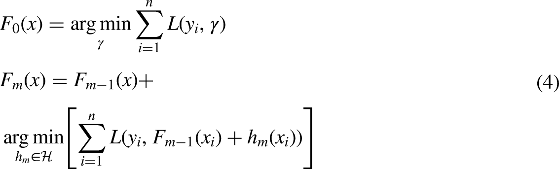
We restrict our method to a reduced form since choosing the appropriate h function at each stage for any loss function L is often a computer optimization challenge. The goal is to solve this minimization issue using the steepest landing step (functional slope descent). The main idea is to use the reduced gradient method in which, by repeating on $F_{m} (x)$ , the local minimum of the Loss function is found. It can be proved that the direction of the maximum descending (most substantial negative derivative) of the loss function to the minimum localized along $F_{m} (x)$ is a function that is reduced by the gradient of the loss function (Chaibi et al., 2021). Hence in Equation (5):

F_{m} (x) = F_{m - 1} (x) - γ \sum_{i = 1}^{n} \nabla_{F_{m - 1}} L (y_{i}, F_{m - 1} (x_{i}))

(5)

Where γ> 0

L (y_{i}, F_{m} (x_{i})) \leq L (y_{i}, F_{m - 1} (x_{i}))

(6)

In addition, we can obtain the optimum by finding the value that the loss function minimizes:

\begin{aligned} γ_{m} = \arg min (\sum_{i = 1}^{n} L (y_{i}, F_{m})) \\ = \arg min (\sum_{i = 1}^{n} L (y_{i}, F_{m - 1} (x_{i}) - γ \nabla_{P_{m - 1}} L (y_{i}, F_{m - 1} (x_{i})))) \end{aligned}

(7)

By considering the continuous mode, where H is a set of arbitrary distinct functions in R, the model can be updated according to the equations mentioned in Equation (8):

\begin{aligned} F_{m} (x) = F_{m - 1} (x) - γ_{m} \sum_{i = 1}^{n} \nabla_{F_{m - 1}} L (y_{i}, F_{m - 1} (x_{i})) \\ γ_{m} = \underset{γ}{\arg min} \sum_{i = 1}^{n} L (y_{i}, F_{m - 1} (x_{i}) - γ \nabla_{F_{m - 1}} L (y_{i}, F_{m - 1} (x_{i}))) \end{aligned}

(8)

According to the current study, machine learning algorithms can recognize complex process patterns. Machine learning techniques were employed to anticipate wind direction, increasing wind power dependability. An ensemble of light gradient boosting machines (Hart et al., 2000) and extra trees measure and predict Basel air wind speed (W.S.).

2.4. Gradient boosting

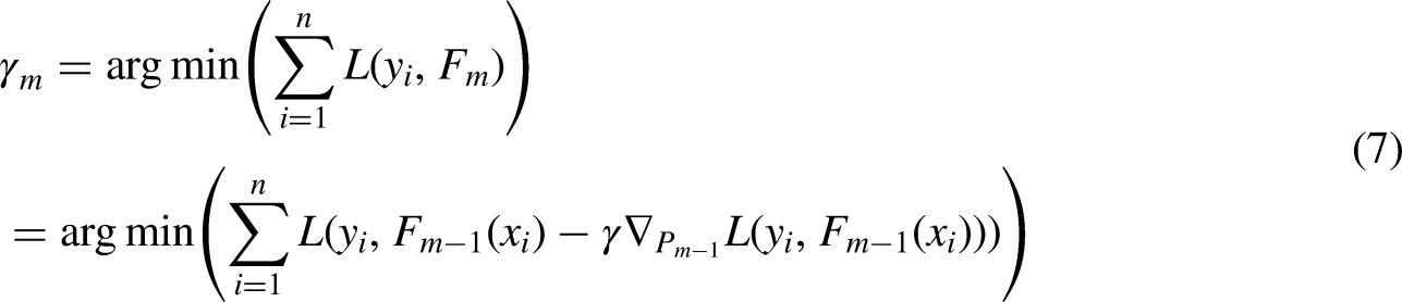
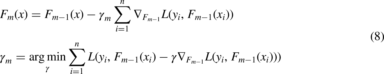
Increasing the gradient in a tree ensemble, new trees are included in the model at each iteration to compensate for flaws. This kind of model is often used when the characteristics of a dataset are very varied. AdaBoost, on the other hand, relies on gradients to identify flaws. The gradient boosting model, on the other hand, is more resistant to outliers. A generalized AdaBoost Gradient Boosting seems to accommodate many loss functions. Loss functions like “Huber” and “absolute” loss functions are often employed in regression models. These loss functions are more resistant to outliers than squared loss functions. Gradient boosting regressor uses the Huber loss function (Chaibi et al., 2021) as a parameter for calculating its losses. Consider purchasing training equipment (where) in addition to a differential loss function (i.e., “deviance” in this case), the expected value. Set up the model as follows Equation (9):

f_{0} (x) = \arg min_{z} \sum_{i = 1}^{i = N} L (y_{i}, z)

(9)

Consider this:

m^{t h}

is the three out of M the number of trees (where

m = 1, 2, 3, \dots, M

m^{t h}

is the tree supplies the negative gradient or residual for each.

g (x_{i}) = \frac{\partial L (y_{i}, f (x_{i}))}{\partial f (x_{i})}

(10)

where

i = 1, 2, 3, \dots, N

. Allow the size of each to be determined

m^{t h}

tree be

J_{m}

, where

R_{j m}

determines the tree area

j = 1, 2, 3, \dots, J_{m}

. Calculate the gradient that is provided for each observation in each tree

θ_{j m} = \arg min_{z} \sum_{}^{} L (y, z + f (x_{i}))

(11)

Apply the gradient from the preceding tree to the new tree's model now. This is the result of

f_{m} (x) = f_{m - 1} (x) + \sum_{j = 1}^{j = J m} l_{j m} . I

(12)

for each x which belongs to the region of that tree (i.e.,

R_{j m}

). The overall output is given by

f_{m} (x)

2.5. Decision tree

The DTR uses a modified version of Quinlan's C4.5 method (Quinlan, 2014). DTR is based on the CART method (Breiman et al., 2017). The DTR, however, presently uses a modified version of Quinlan's C4.5 method (Quinlan, 2014).

The following are the two primary topics that will be covered in this essay:

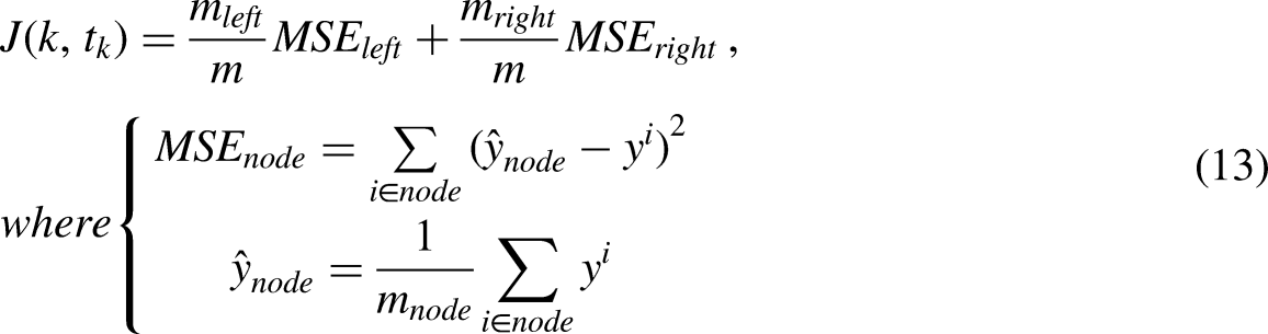
1. Node Structure: Each node guides the prediction process by storing properties that determine the tree structure.

2. Node Split: Node split identifies the feature and threshold value needed to divide a node. The node is divided for a feature and threshold value that minimizes the cost function after computing the CART cost function for various features k and thresholds t_k in Equation (13).

\begin{aligned} J (k, t_{k}) = \frac{m_{l e f t}}{m} M S E_{l e f t} + \frac{m_{r i g h t}}{m} M S E_{r i g h t}, \\ w h e r e {\begin{matrix} M S E_{n o d e} = \sum_{i \in n o d e} {({\hat{y}}_{n o d e} - y^{i})}^{2} \\ {\hat{y}}_{n o d e} = \frac{1}{m_{n o d e}} \sum_{i \in n o d e} y^{i} \end{matrix} \end{aligned}

(13)

2.6. Ada boost

Boosting comes in handy when everything else fails. Nowadays, many users employ XGBoost, LightGBM, or CatBoost to win Kaggle or Hackathon events. It's the first step into the realm of Boosting using AdaBoostIt was one of the earliest boosting methods used in solving practice. Adaboost makes it possible to create a single “strong classifier” out of numerous “weak classifiers.”

2.7. Ridge

In situations when the independent variables are strongly correlated, ridge regression is a technique for estimating the coefficients of multiple regression models. It has been used in various disciplines, including engineering, chemistry, and econometrics. Overfitting is an issue that ridge regression addresses since squared error regression alone cannot distinguish between significant and unimportant characteristics, using all of them instead, resulting in overfitting. Ridge regression introduces a small amount of bias to match the model to the actual values of the data.

3. Methods

3.1. Data preparation

Data (https://www.kaggle.com/datasets/alexmoskvin1/windturbinescada) contains 85,066 rows × 10 columns features of data as shown below:

Windspeed, power, wind direction Angle, rtr_rpm, pitch Angle, generation, wheel hub temperature, ambient temperature, Tower bottom ambient temperature, failure time.

Data were recorded from March 01, 2020, 00:00:00 to December 31, t2020, 23:50:00.

3.2. Evolution process

Tenfold in cross-validation (Malakouti and Ghiasi, 2022; Malakouti and Ghiasi, 2022), the model is evaluated and trained using a variety of data points across a few rounds. Most people use it when they're trying to anticipate something and want to see how well a model works in real-world situations. With 60% of the data being used for training and 40% for validation and testing, we use the cross-validation technique.

4. Results and discussion

Residual plots are used to test the assumptions of an OLS linear regression model. Fitted values or another variable are shown on the x-axis, while the remaining values are plotted on the y-axis. When fitting a regression model, it is essential to look at the remaining graphs. Figures 1 to 7 give these graphs for the power predictive and actual power with extra tree, random forest, light gradient boosting machine, gradient boosting regressor, decision tree, Ada Boost, and ridge.

Figure 1.

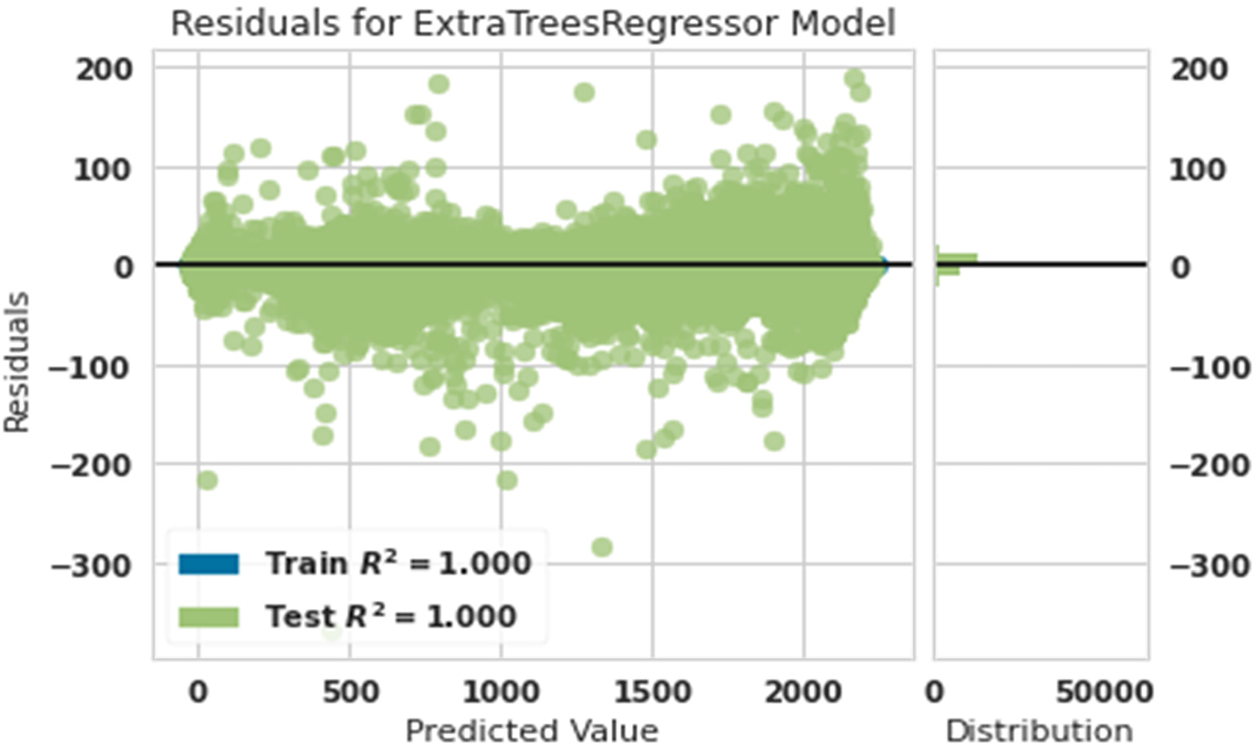
Residual diagram of predicted power and actual power with extra tree.

Figure 2.

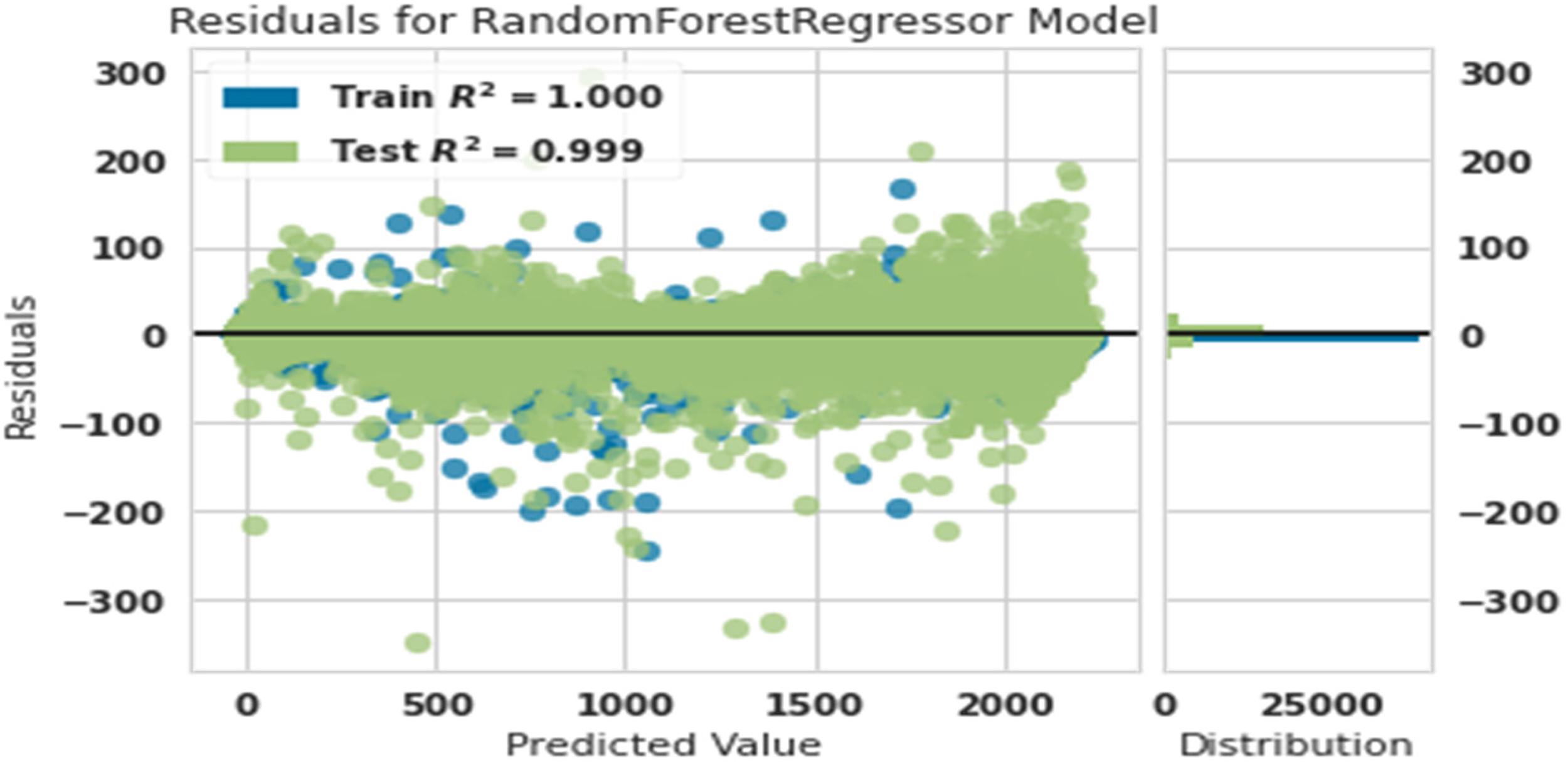
Residual diagram of predicted power and actual power with random forest.

Figure 3.

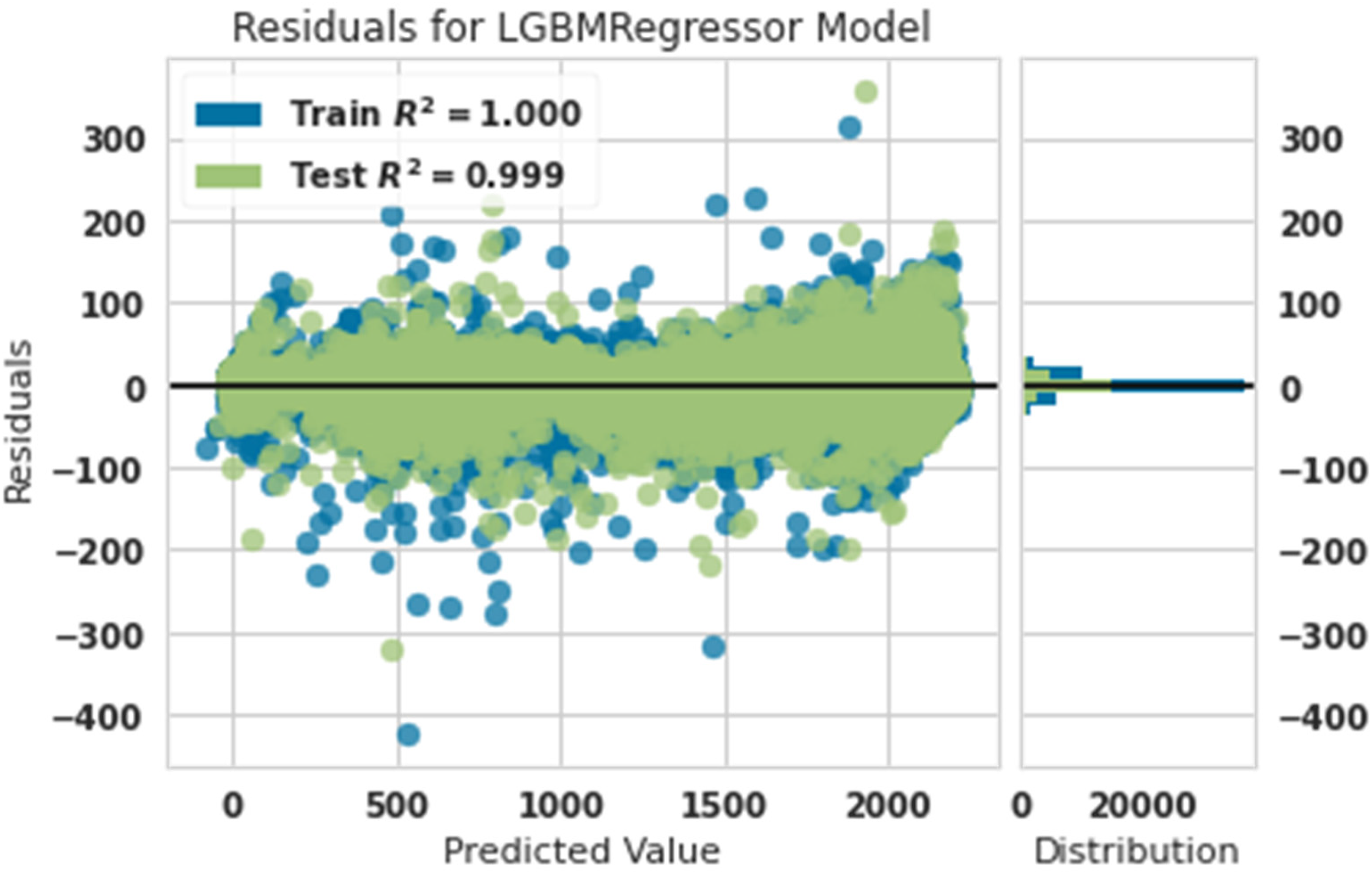
Residual diagram of predicted power and actual power with lightgbm.

Figure 4.

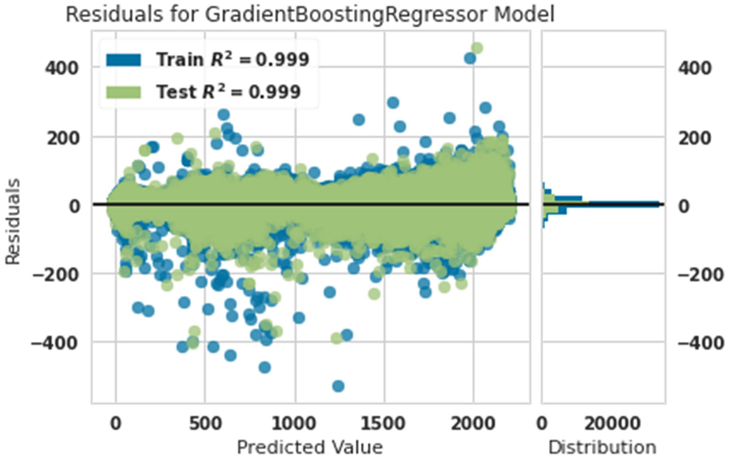
Residual diagram of predicted power and actual power with gradient boosting regressor.

Figure 5.

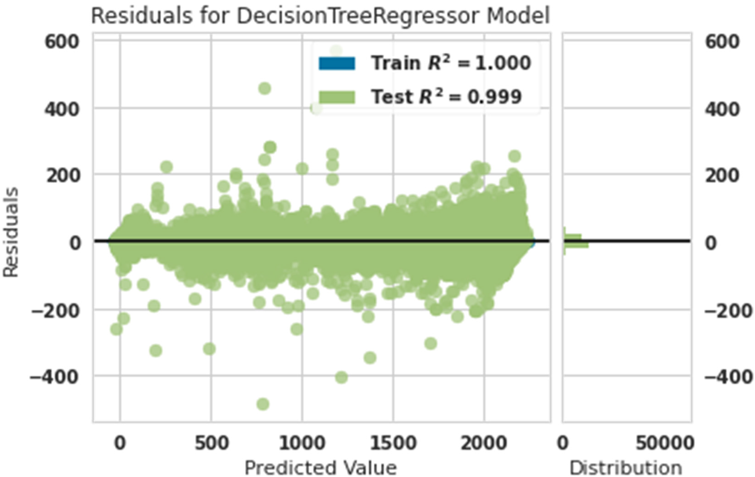
Residual diagram of predicted power and actual power with decision tree.

Figure 6.

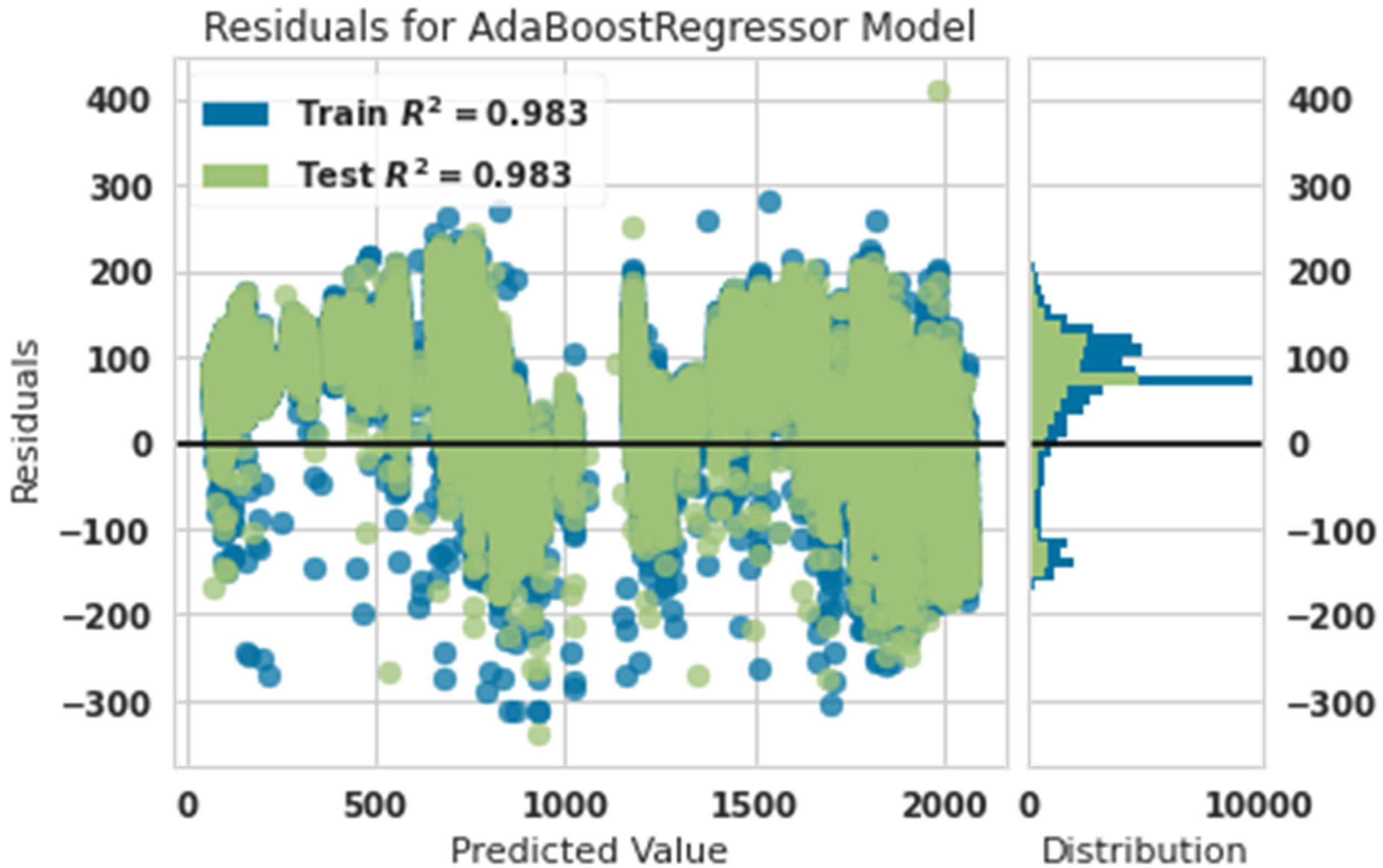
Residual diagram of predicted power and actual power with Ada Boost.

Figure 7.

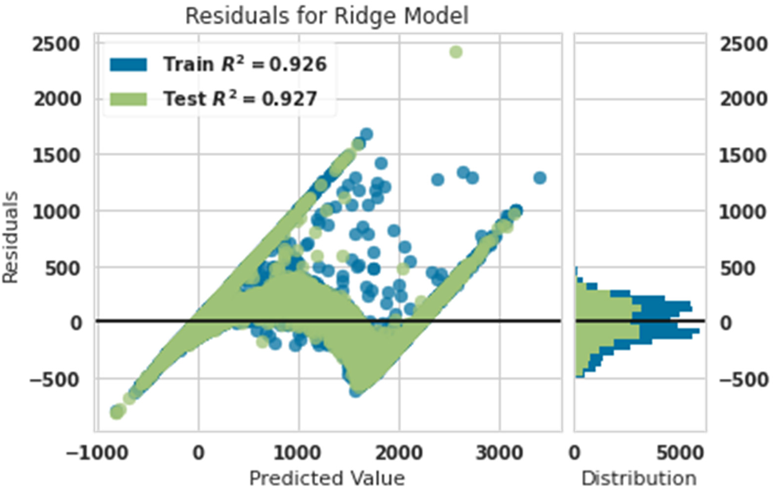
Residual diagram of predicted power and actual power with ridge.

Figure 1 shows that the training and test data matched 100% accuracy. This showed that the extra tree algorithm was the most powerful in predicting the production power of the turbine.

Figure 2 shows that the training data were matched with 100% accuracy, and test data were matched with 99% accuracy. This showed that the random forest algorithm was robust in predicting the production power of the turbine.

Figure 3 shows that the training data were matched with 100% accuracy, and test data were matched with 99% accuracy. This showed that the light gradient boosting machine algorithm was robust in predicting the production power of the turbine.

Figure 4 shows that the training data were matched with 99% accuracy, and test data were matched with 99% accuracy. This showed that the gradient boosting algorithm was robust in predicting the production power of the turbine. This algorithm is a little weaker than the light gradient boosting machine and random forest algorithms, and this claim is 99% accurate to the training data. At the same time, the light gradient boosting machine and random forest algorithms had 100% accuracy in the training data.

Figure 5 shows that the training data were matched with 100% accuracy, and test data were matched with 99% accuracy. This showed that the decision tree algorithm was a robust algorithm for predicting the production power of the turbine. This algorithm is a little stronger than the gradient boosting algorithm, and this claim is 100% accurate to the training data. At the same time, the gradient boosting algorithm had 99% accuracy in the training data.

Figure 6 showed that the training data were matched with 98.3% accuracy, and test data were matched with 98.3% accuracy. This showed that the Ada Boost algorithm was a robust algorithm for predicting the production power of the turbine. This algorithm is weaker than the gradient boosting algorithm, decision tree, extra tree, random forest, and lightgbm. This claim is 100% accurate of the training data. In contrast, the gradient boosting algorithm had 99% accuracy in the training data.

Figure 7 shows that the training data were matched with 92.6% accuracy, and test data were matched with 92.7% accuracy. This showed that the ridge algorithm was not very powerful in predicting the production power of the turbine. This algorithm is the weakest of other algorithms.

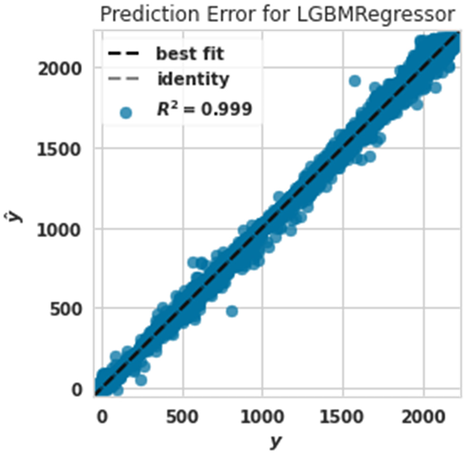
The prediction error plot diagram shows the fundamental goals of the data set against the predicted values generated by our model. This allows us to see how much variance there is in the model. Figures 8 to 14 show the prediction error plot diagram for the predicted and actual power capabilities. As you can see, the powers that be were predicted correctly. Identified by us (identity) were placed on top of each other.

Figure 8.

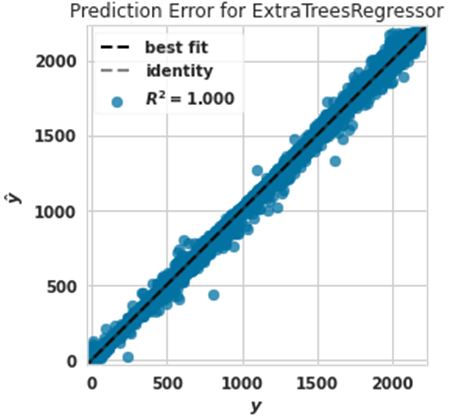
Power prediction error diagram with extra tree.

Figure 9.

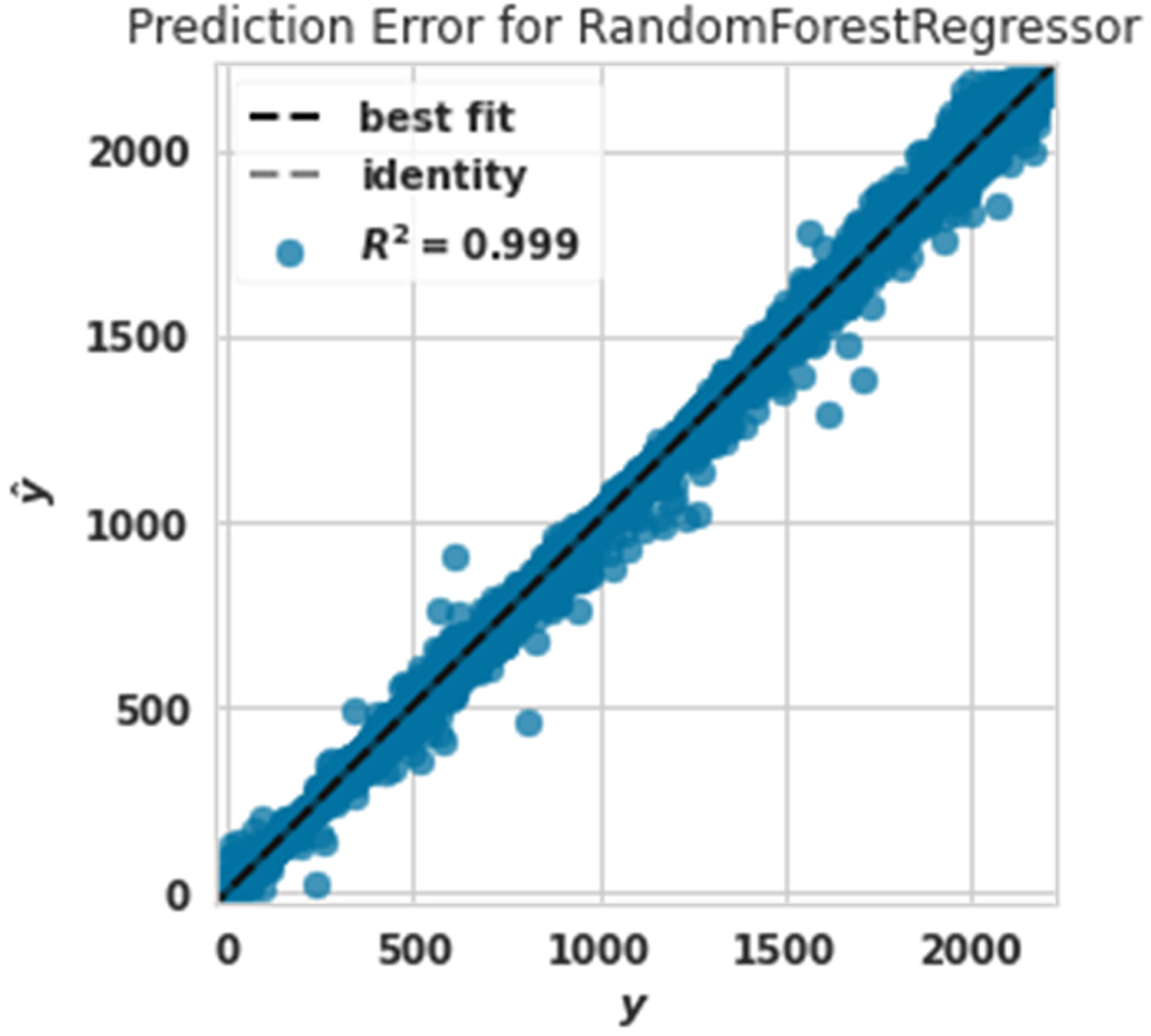
Power prediction error diagram with random forest.

Figure 10.

Power prediction error diagram with lightgbm.

Figure 11.

Power prediction error diagram with gradient boosting regressor.

Figure 12.

Power prediction error diagram with decision tree.

Figure 13.

Power prediction error diagram with Ada Boost.

Figure 14.

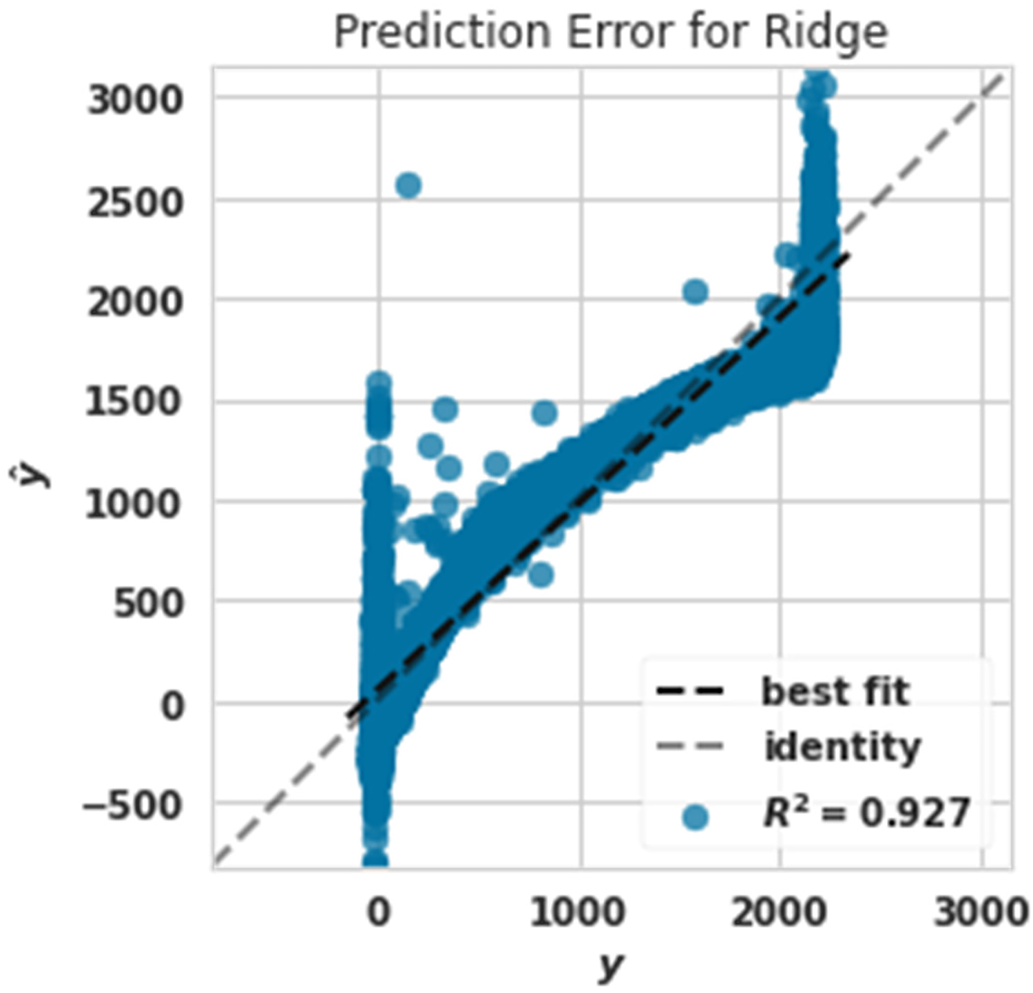
Power prediction error diagram with ridge.

The power prediction error diagram with the extra tree is shown in Figure 8. The R2 evaluation criterion in this algorithm was assigned the value of 1. The extra tree algorithm had the best performance in predicting production power. This claim can be proven by comparing Figures 8 to 14.

Figure 9 shows the power prediction error diagram with a Random forest The evaluation criterion of R2 in this algorithm was 0.999. The random forest algorithm had the best performance after the extra tree algorithm in predicting production power.

The evaluation criterion of R2 in this algorithm was 0.999. Lightgbm algorithm had the best performance after the extra tree algorithm in predicting production power.

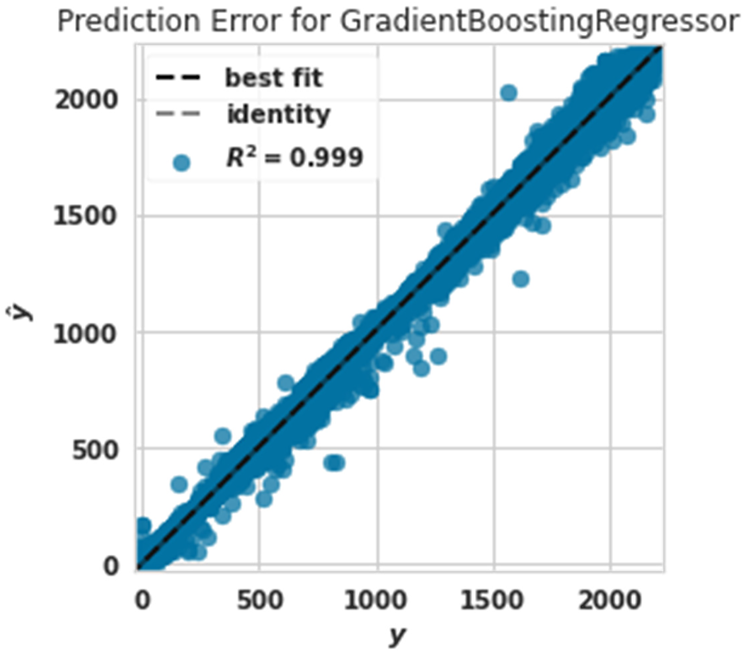
Figure 11 shows the Power prediction error diagram with a gradient boosting regressor. The evaluation criterion of R2 in this algorithm was 0.999. The gradient boosting regressor algorithm had the best performance after the extra tree algorithm predicting production power.

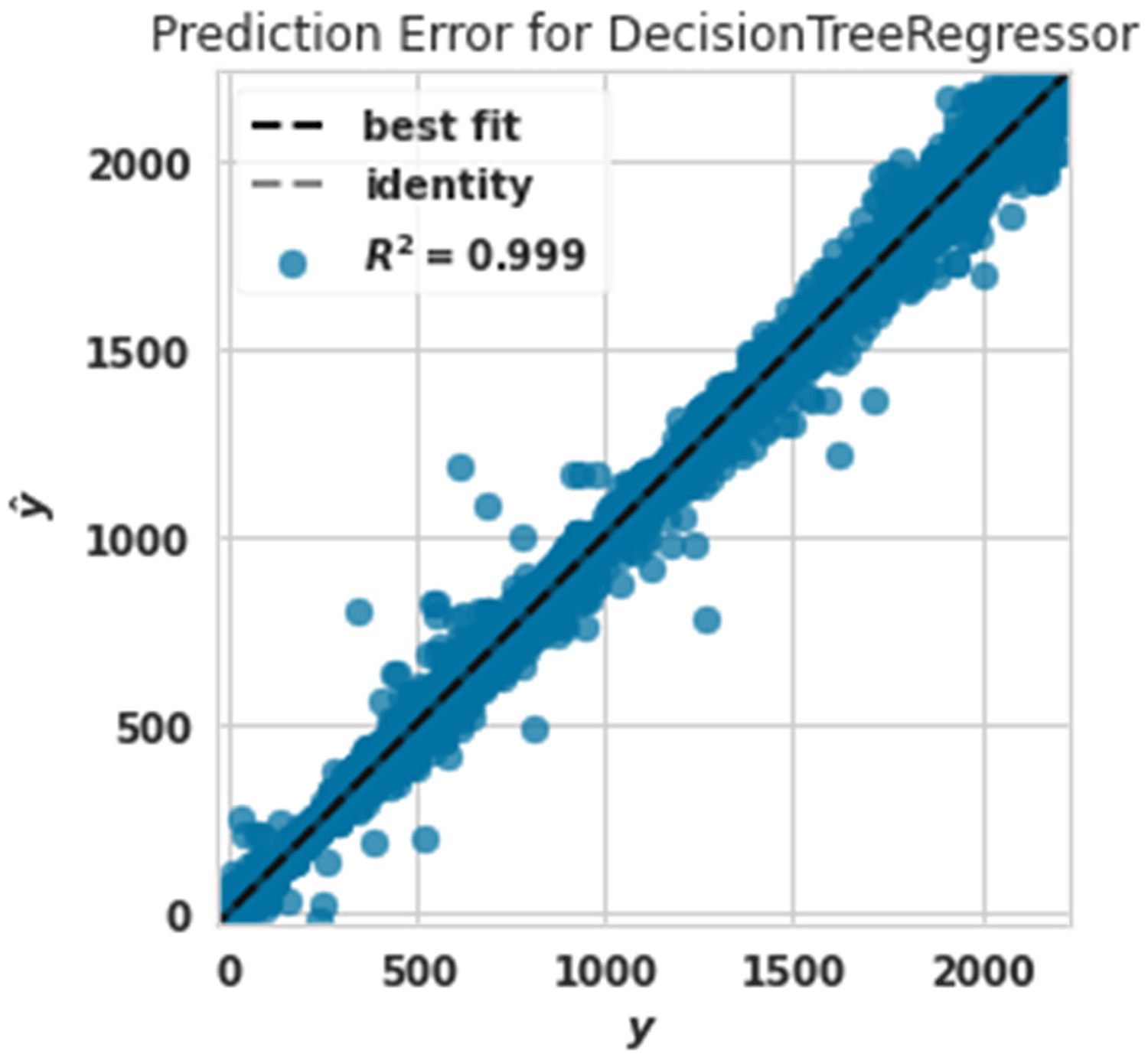
Figure 12 shows the Power prediction error diagram with a decision tree regressor. The evaluation criterion of R2 in this algorithm was 0.999. The decision tree regressor algorithm had the best performance in predicting production power after the extra tree algorithm.

By comparing the results of Figures 9 to 12, we realized that random forest, LightGBM, gradient boosting, and decision tree regressor algorithms had very similar performances predicting wind turbine production power.

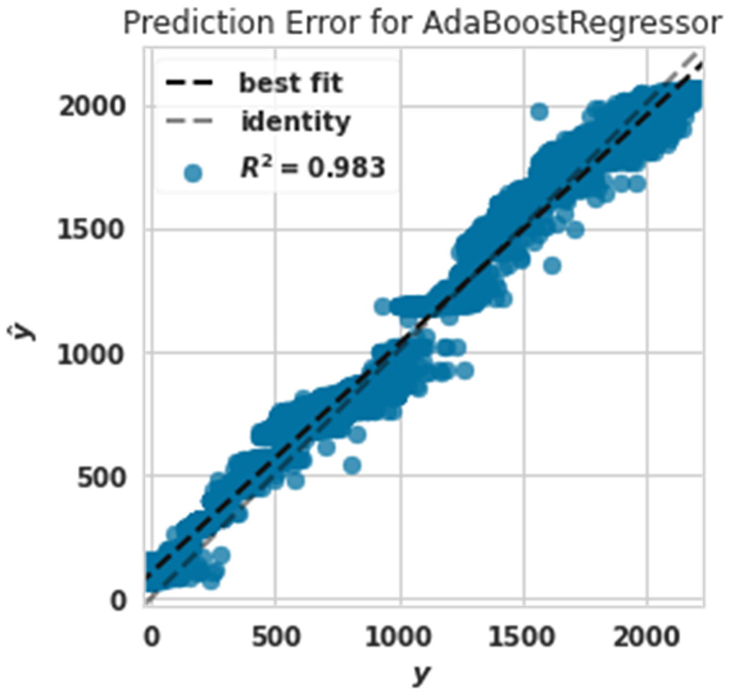
Figures 13 and 14 show the weak performance of Ada Boost and ridge algorithms compared to other algorithms. Figure 14 shows that the ridge algorithm predicted very low and high powers poorly. This claim is seen in Figure 14. Low powers were poorly predicted because between two values of 0–500, Figure 14 is drawn, and very high powers are drawn between 2000 and 3000, according to Figure 8, which was related to the extra tree. The algorithm realized that the actual and predicted values should be between 0 and 2500.

Figures 15–21 show the actual measured and predicted power with models in this article for 1 day. In these figures, every 10 min during 24 h a day, the power predicted by the proposed algorithms and the actual amount of power are recorded and brought together in one format. As it turns out, the power is well predicted by all models. Figures 16 to 19 show actual and predicted power for 1 day with random forest, lightgbm, gradient boosting regressor, and decision tree. Algorithms random forest, lightgbm, gradient boosting regressor, and decision tree had similar performance in predicting wind turbine production power with the difference that the decision tree algorithm had the lowest speed, and the lightgbm algorithm had good accuracy in addition to the low speed to run. Ada Boost and ridge algorithms did not perform well compared to other algorithms. These two algorithms were slower to execute than extra tree and random forest, while they had poor results predicting production capacity.

Figure 15.

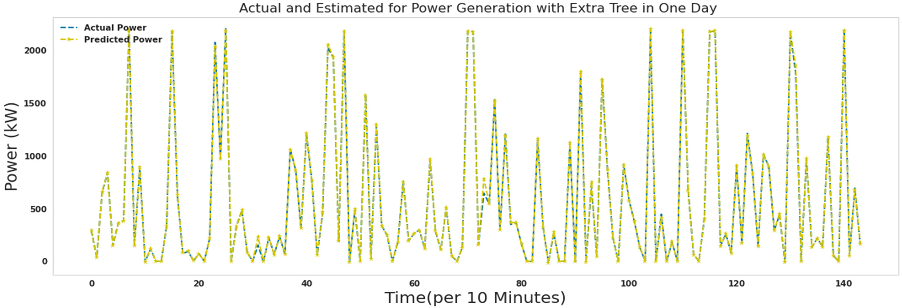
Actual and predicted power for 1 day with an extra tree.

Figure 16.

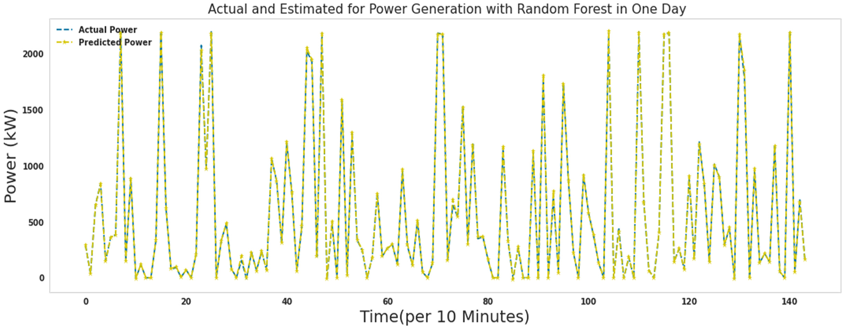
Actual and predicted power for 1 day with random forest.

Figure 17.

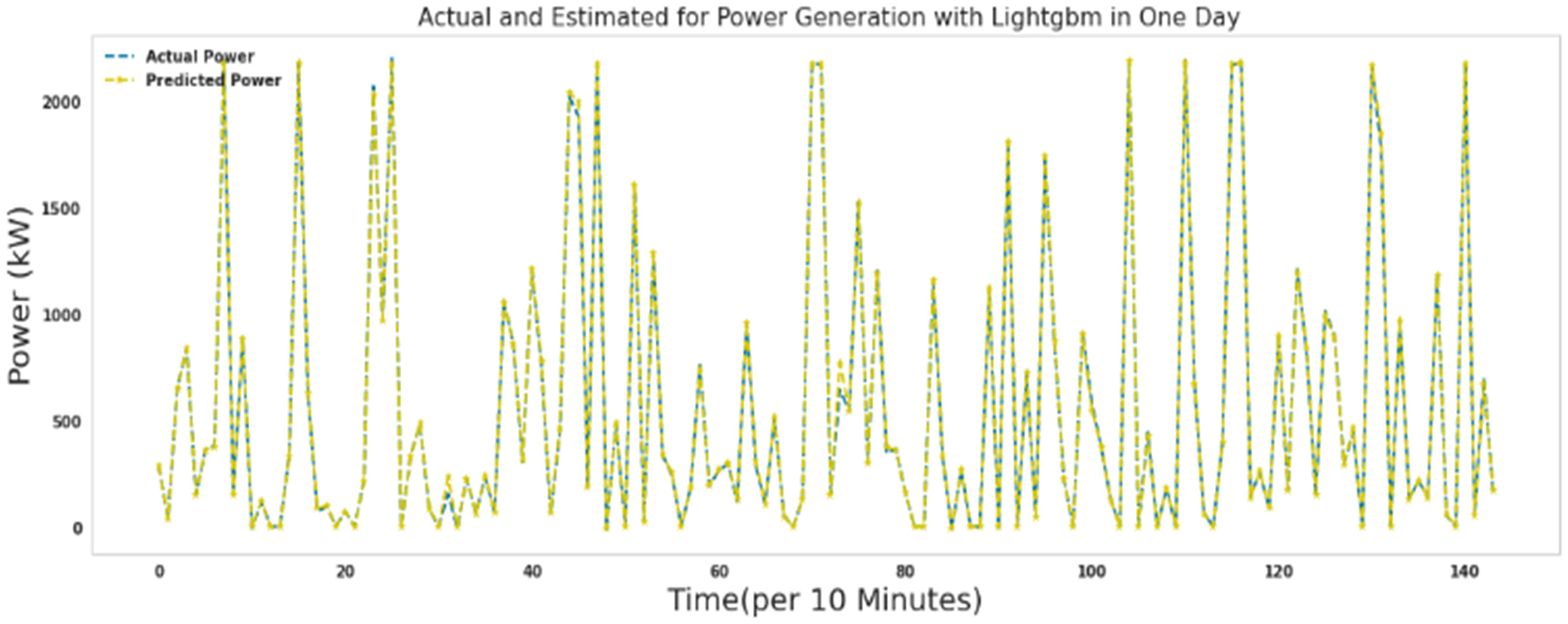
Actual and predicted power for 1 day with lightgbm.

Figure 18.

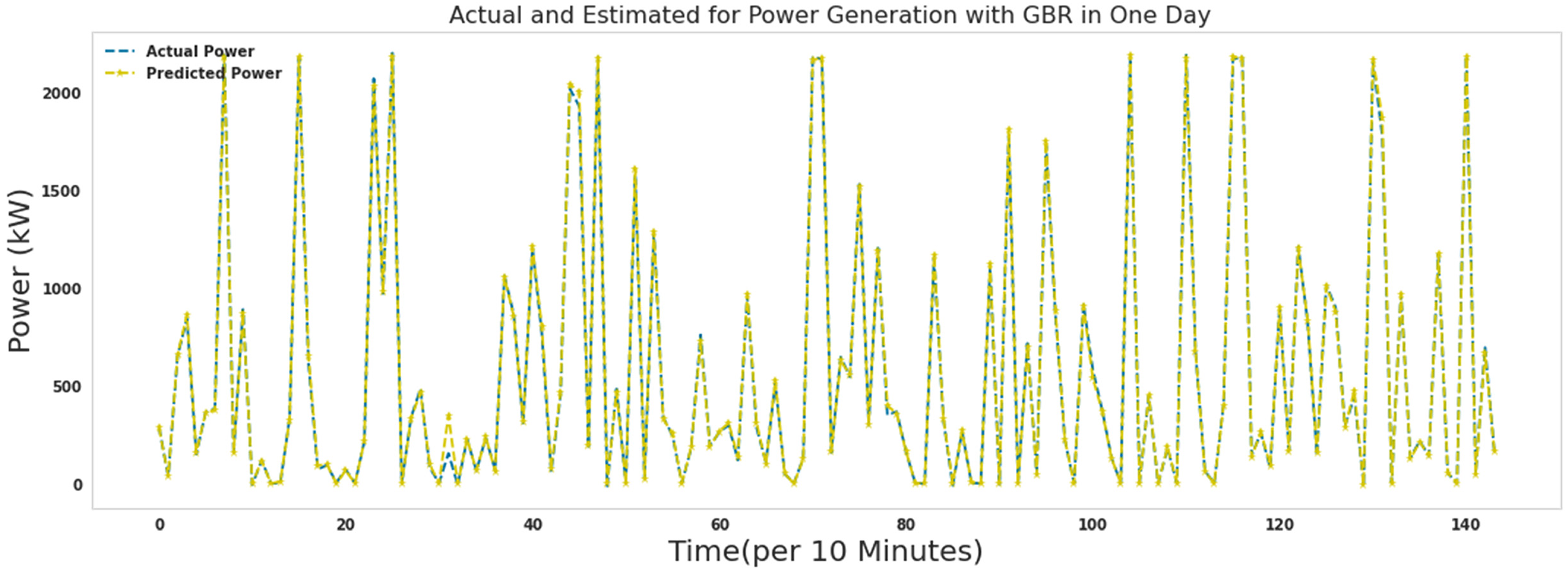
Actual and predicted power for 1 day with gradient boosting regressor.

Figure 19.

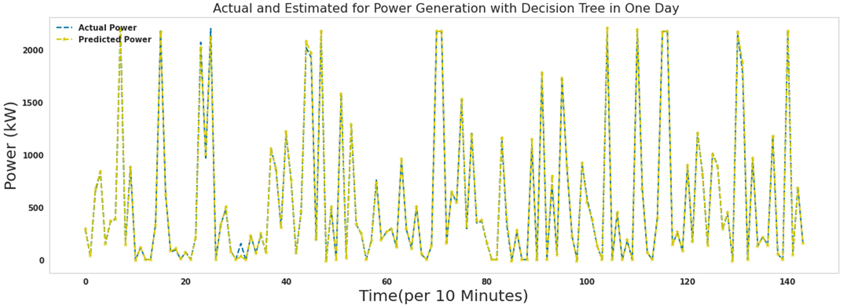
Actual and predicted power for 1 day with decision tree.

Figure 20.

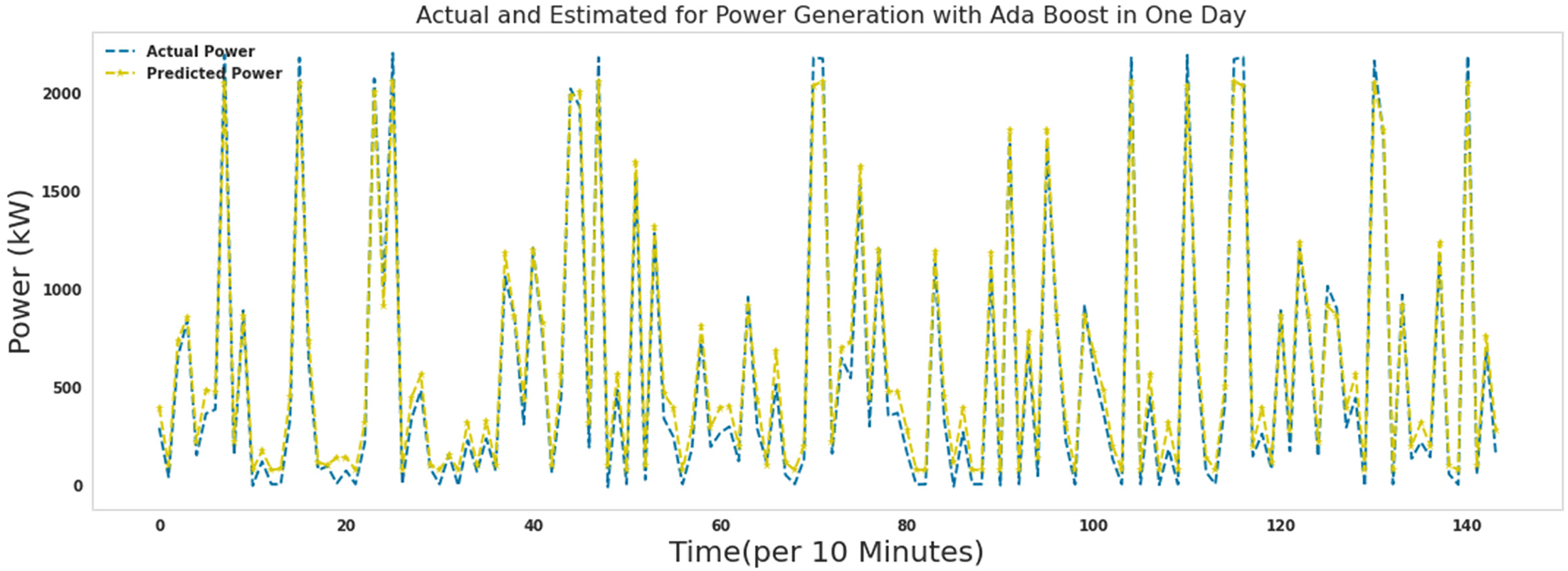
Actual and predicted power for 1 day with Ada Boost.

Figure 21.

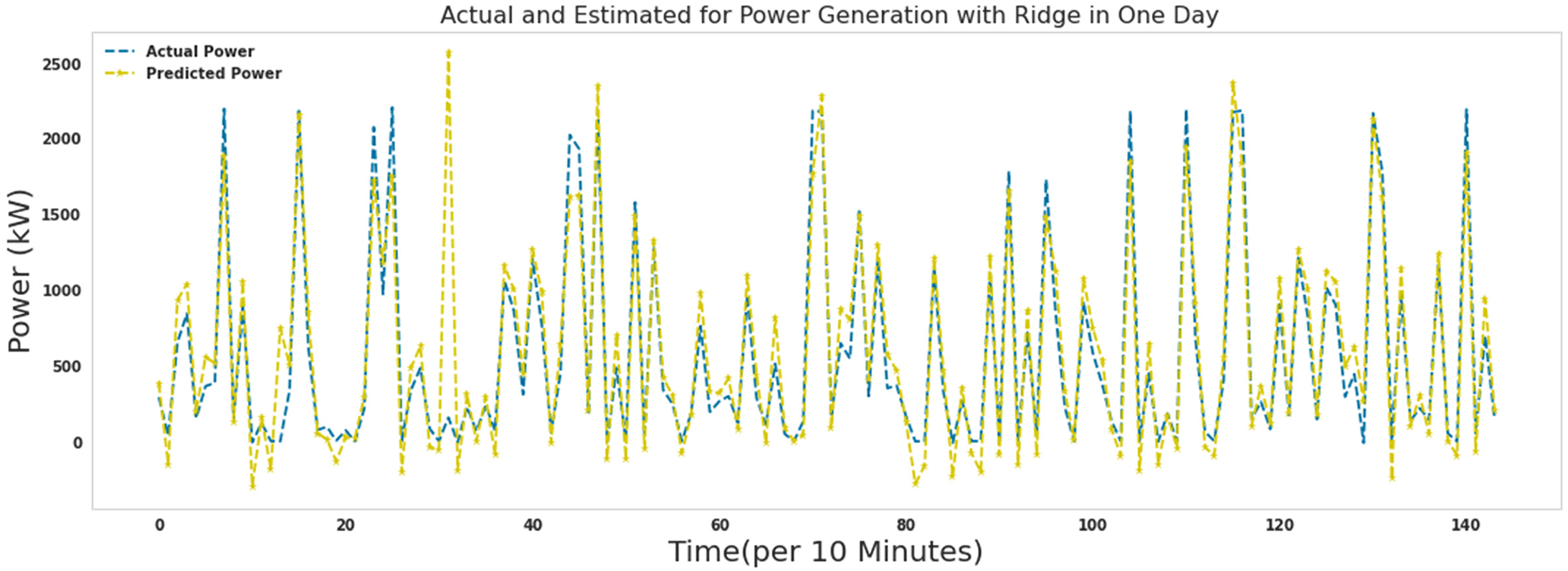
Actual and predicted power for 1 day with ridge.

Figure 22 shows the error between actual and predicted power for 1 day with an extra tree. As it is known, most of the errors assigned by the extra tree algorithm in predicting the production power of the turbine are close to zero. The extra tree algorithm needed 150 s to run.

Figure 22.

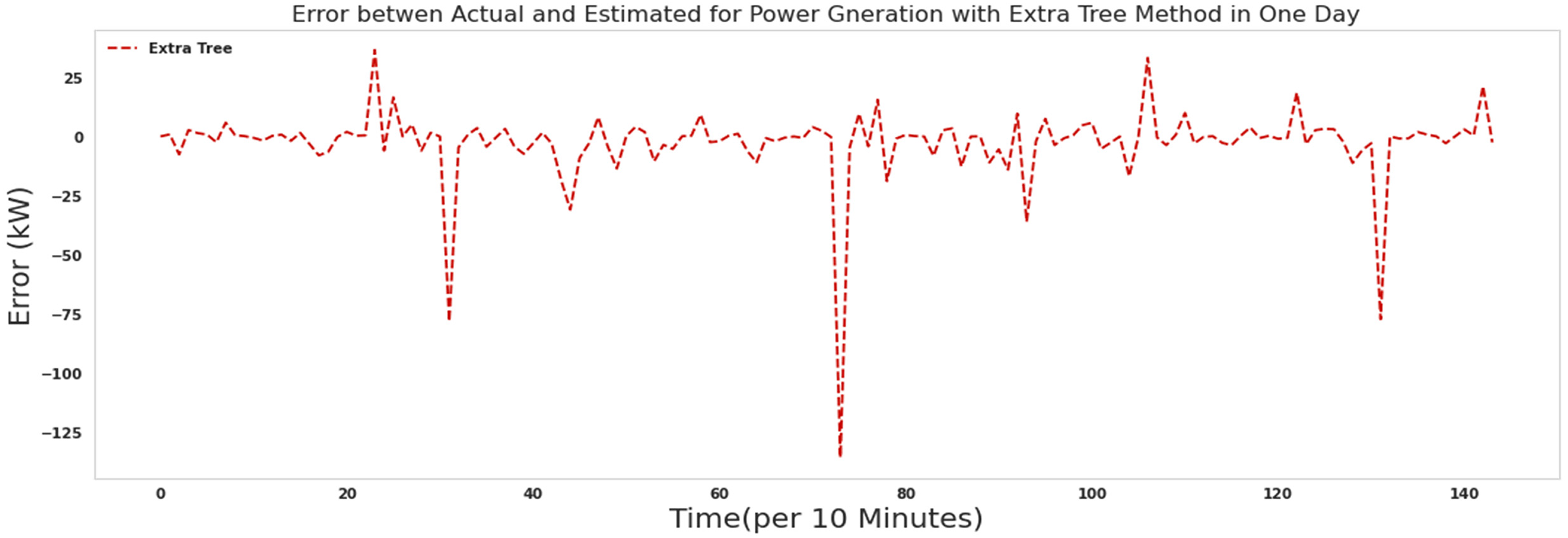
The error between actual and predicted power for 1 day with an extra tree.

As it is known, most of the errors assigned by the Random forest algorithm in predicting the production power of the turbine are close to zero. Comparing the performance of the extra tree algorithm and the random forest algorithm, the errors in the extra tree algorithm were closer to zero. The random forest algorithm needed 340 s to run.

As it is known, most of the errors assigned by the lightgbm algorithm in predicting the production power of the turbine are close to zero. Comparing the performance of the extra tree algorithm and the lightgbm algorithm, the errors in the extra tree algorithm were closer to zero. The lightgbm algorithm took 53 s to run.

As it is known, most of the errors assigned by the decision tree algorithm in predicting the production power of the turbine are close to zero. Comparing the performance of the extra tree algorithm and the decision tree algorithm, the errors in the extra tree algorithm were closer to zero. The decision tree algorithm needed 5.8 s to run.

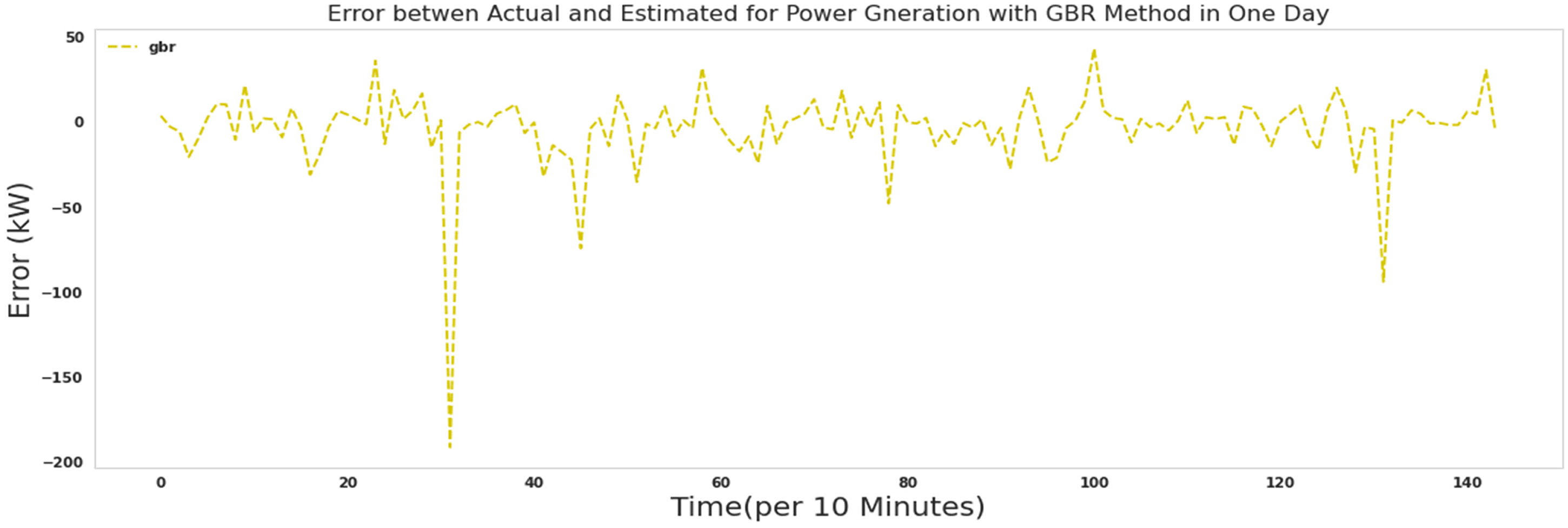
As it is known, most of the errors assigned by the gradient boosting regressor algorithm in predicting the production power of the turbine are close to zero. Comparing the performance of the Extra tree algorithm and the gradient boosting regressor algorithm, the errors in the Extra tree algorithm were closer to zero. The gradient boosting regressor algorithm needed 92 s to run.

As it is known, the errors assigned by the Ada Boost algorithm in predicting the production power of the turbine were assigned more values when comparing the performance of the Extra tree algorithm. The Ada Boost algorithm needed 39 s to run.

As it is known, the ridge algorithm's errors in predicting the turbine's production power were assigned more values when comparing the performance of the Extra tree algorithm. The ridge algorithm needed 35 s to run.

Figures 22 to 28 show the error between the actual and predicted production power in Figures 15 to 21. Figures 22 to 28 show the error between the actual and predicted production power in Figures 15 to 21. Figures 23 to 26 show the similar performance of random forest, lightgbm, decision tree, and gradient boosting regressor algorithms.

Figure 23.

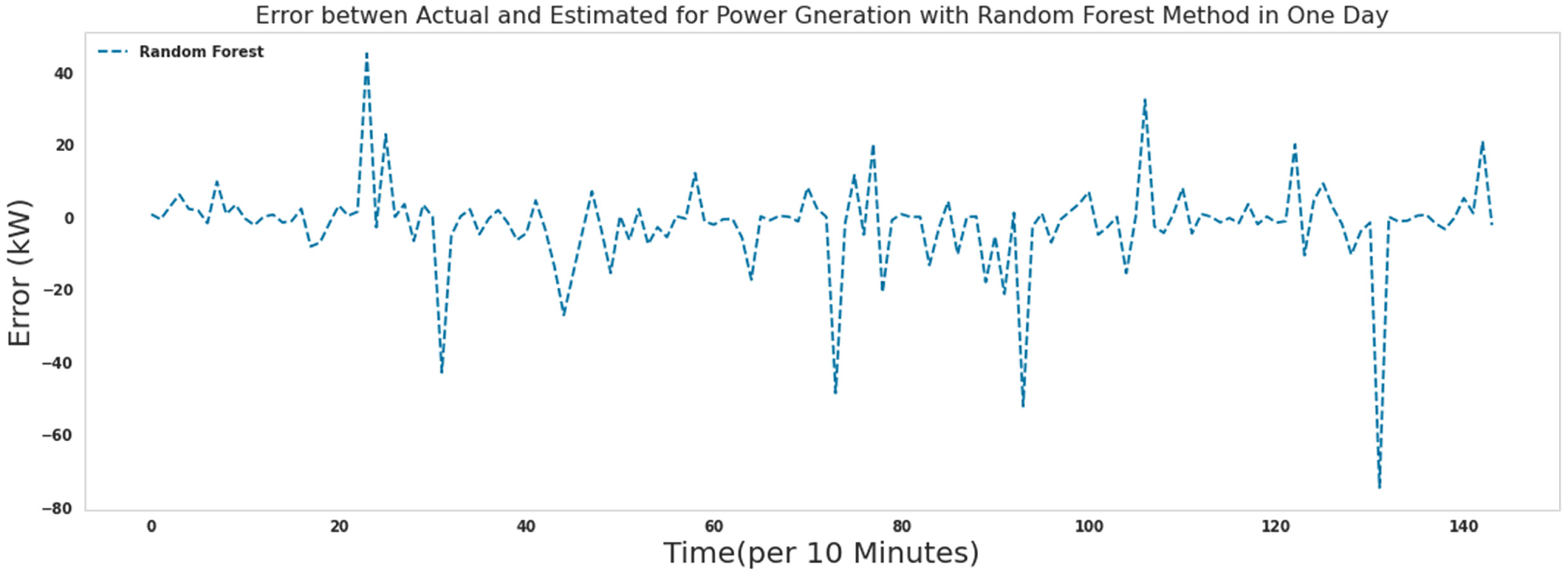
The error between actual and predicted power for 1 day with random forest.

Figure 24.

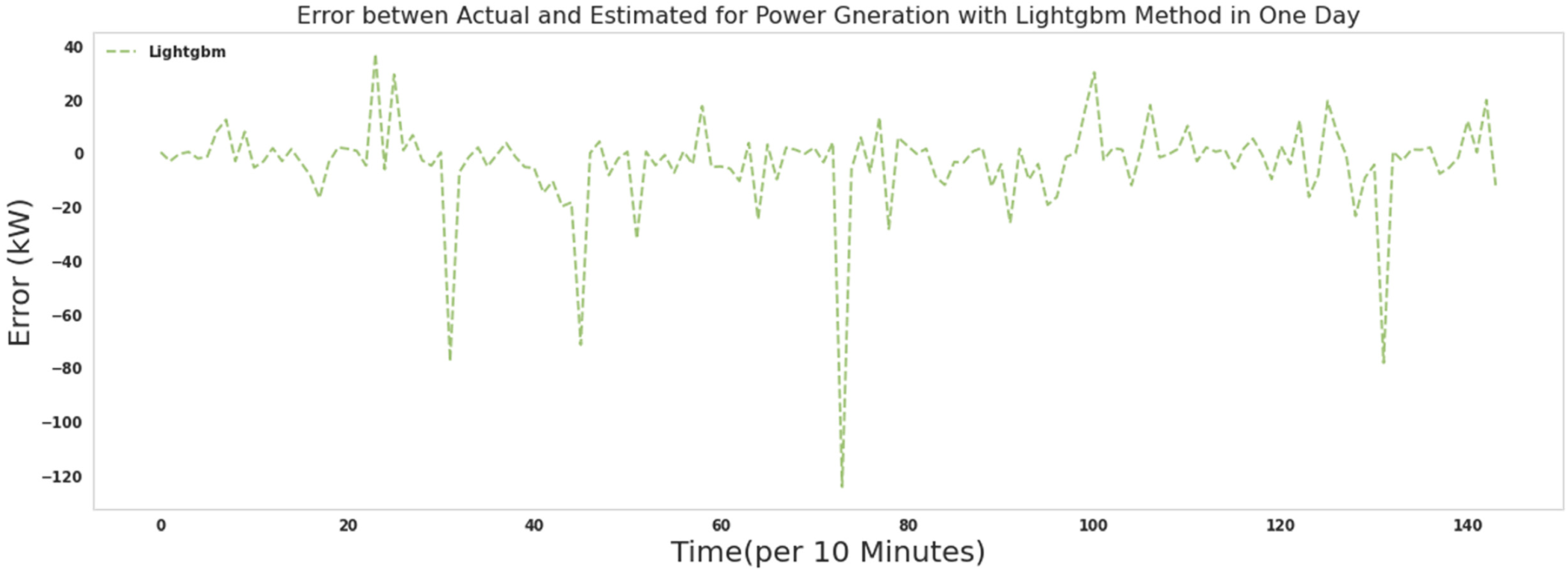
The error between Actual and predicted power for 1 day with lightgbm.

Figure 25.

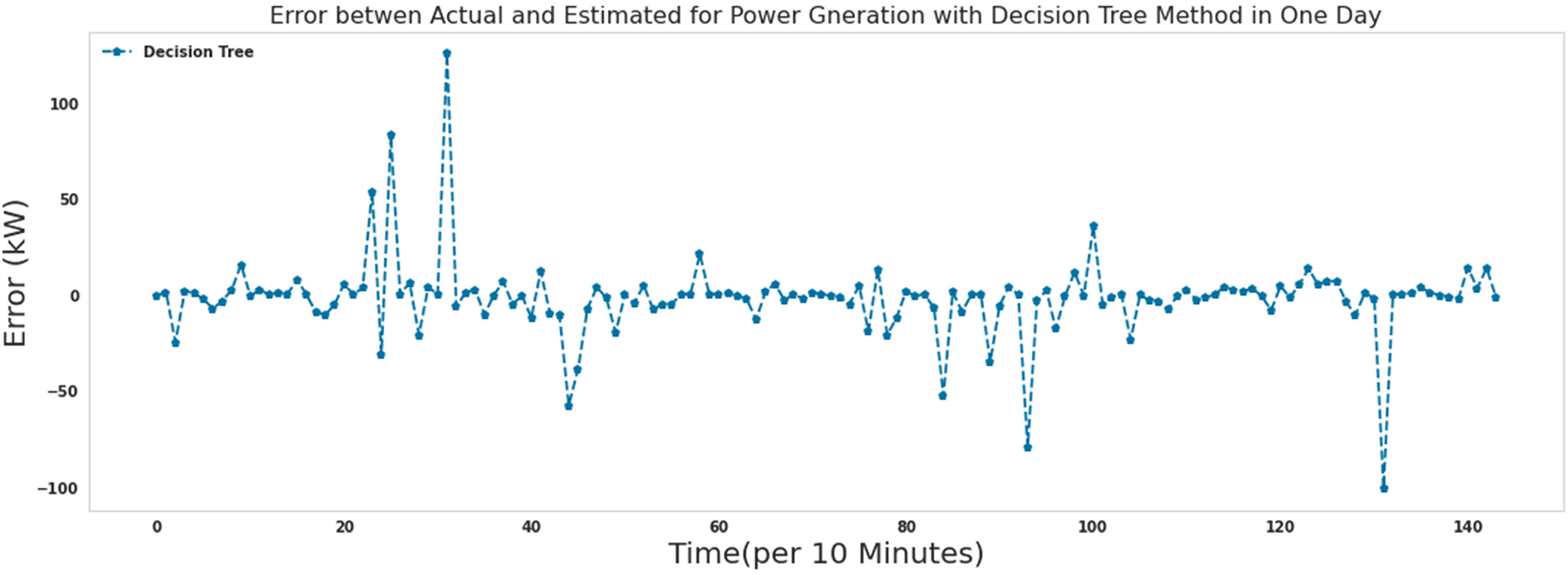
The error between Actual and predicted power for 1 day with the decision tree.

Figure 26.

The error between actual and predicted power for 1 day with gradient boosting regressor.

Figure 27.

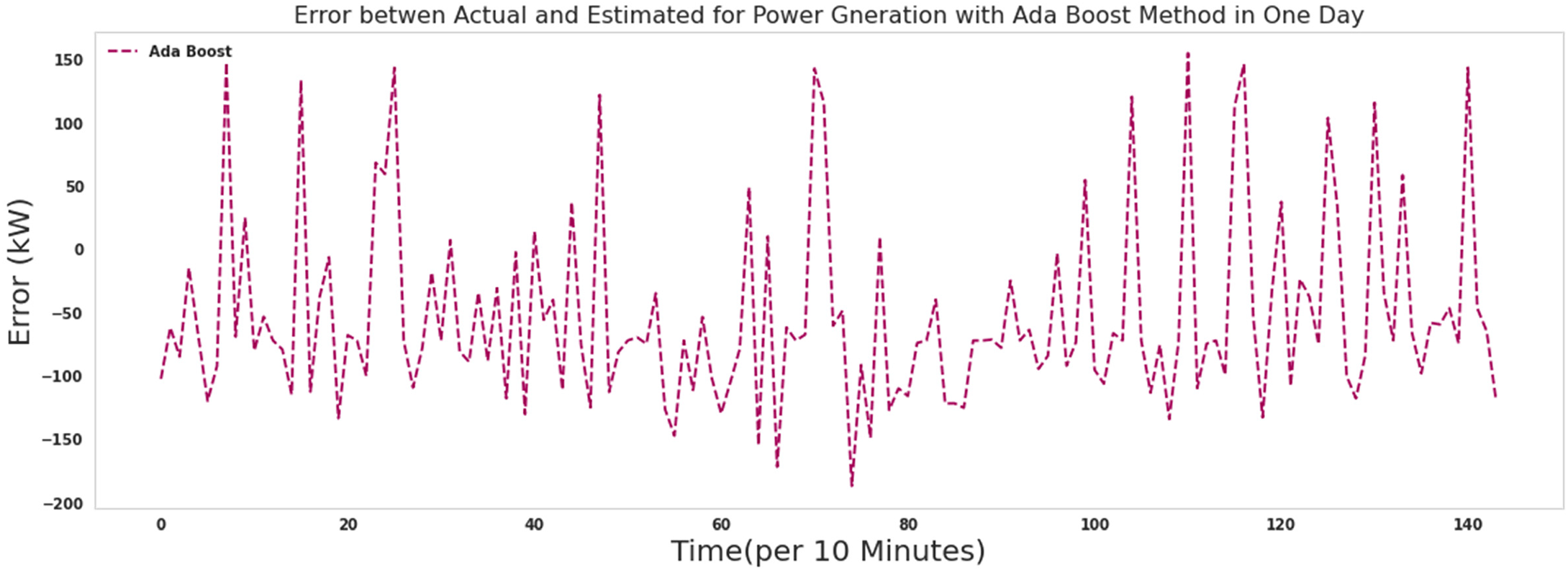
The error between Actual and predicted power for 1 day with Ada Boost.

Figure 28.

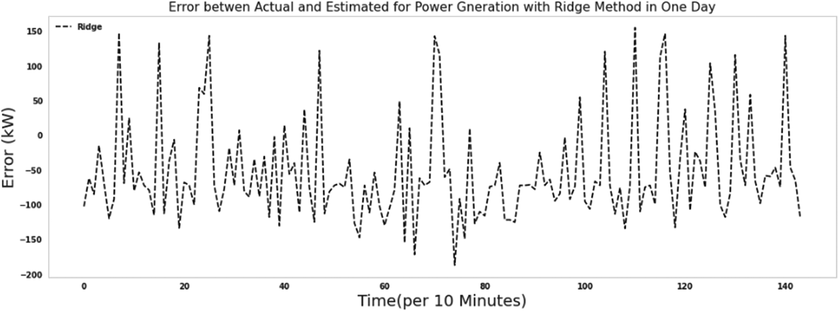
The error between actual and predicted power for 1 day with ridge.

It is possible to measure the performance of algorithms using indices such as MSE, MAE, and the root mean square error (RMSE). The definition of these indexes follows:

\begin{aligned} M S E = \frac{1}{n} \sum_{i = 1}^{n} (W_{i} - {\hat{W}}_{i})^{2} \\ R M S E = \sqrt{\frac{1}{n} \sum_{i = 1}^{n} (W_{i} - {\hat{W}}_{i})^{2}} \\ M A E = \frac{\sum_{i = 1}^{n} | W_{i} - {\hat{W}}_{i} |}{n} \end{aligned}

(14)

Where

W_{i}

is the actual value, and

\hat{W_{i}}

is the predicted value.

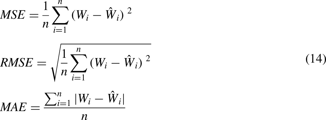
According to Table 1, the criteria for evaluating the production capacity of the wind farm were given. A very acceptable value of 17.22 was obtained for assessing the mean squared error for an extra tree. The evaluation criterion of R2 in regression tasks is the same as the accuracy in classification tasks.

Table 1.

Evaluation criteria R2, mean square error, root mean square error, mean absolute error, and time for test data in power prediction

model	MAE	MSE	RMSE	R ²	Time (s)
Extra tree	7.97	297.53	17.22	1	150
Random forest	8.22	336.53	18.31	0.99	340
Light gradient boosting machine	9.83	364.65	19.07	0.99	53
Gradient boosting regressor	14.79	693.38	26.31	0.99	92
Decision tree	11.48	644.35	25.34	0.99	5.8
Ada Boost	88.96	9639.7	98.13	0.983	39
Ridge	161.68	41275.50	203.15	0.927	35

5. Conclusion

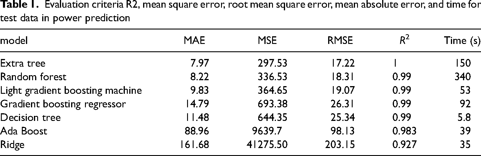
Due to the reduction of fossil fuels and the pollution of fossil fuels to produce power, renewable energy should be replaced by non-renewable energy. Therefore, in the not-too-distant future, we will see the replacement of renewable energy production capacity with the production capacity of fossil fuel power plants. This paper studied a wind farm. With the help of extra tree, light gradient boosting machine, gradient boosting regressor, decision tree, Ada Boost, and ridge power generation was predicted. And in less than a minute, we could predict the wind farm production capacity with a light gradient boosting machine with accurate values. The light gradient boosting machine algorithm was highly accurate with less execution time than other algorithms. Table 1 is proof of this claim. In the final word. The extra tree algorithm had the best results among all algorithms. The extra tree and light gradient boosting machine algorithms obtained the best results compared to other algorithms and the excellent results of these two algorithms. They also had a low execution time. According to this article, we can safely replace the production capacity of wind farms with the production capacity of fossil fuel power plants or use it next to fossil fuel power plants and not be afraid of the nature of wind escape because we can predict it well.

Footnotes

Acknowledgments

I thank my God and my family.

Availability of data and material

https://www.kaggle.com/datasets/alexmoskvin1/windturbinescada

Authors’ contributions

Seyed Matin Malakouti performed all the simulations and wrote the text of the article.

Declaration of conflicting interests

The author(s) declared no potential conflicts of interest with respect to the research, authorship, and/or publication of this article.

Funding

The author(s) received no financial support for the research, authorship, and/or publication of this article.

ORCID iD

Seyed Matin Malakouti

References

Arun Kumar

SVV

Nagababu

Kumar

(2019) Comparative study of offshore winds and wind energy production derived from multiple scatterometers and met buoys. Energy 185: 599e611.

Athari

Wang

(2018) Impacts of wind power uncertainty on grid vulnerability to cascading overload failures. IEEE Transactions on Sustainable Energy 9: 128–137.

Barros

Cerqueira

Soares

(2021) Empirical study on the impact of different sets of parameters of gradient boosting algorithms for time-series forecasting with LightGBM. In: Pacific Rim International Conference on Artificial Intelligence. Cham: Springer, pp. 454–465.

Bhattacharyya

Vyas

(2021) Data-driven model-based rate decline prediction in unconventional eagle ford shale oil wells. Petroleum Science and Technology 1: 401–422.

Bhattacharyya

Vyas

(2022) Machine learning based rate decline prediction in unconventional reservoirs. Upstream Oil and Gas Technology 8: 100064.

Breiman

Friedman

Olshen

, et al. (2017 Oct 19) Classification and regression trees. Routledge.

Caglayan

Ryberg

Heinrichs

, et al. (2019) The techno-economic potential of offshore wind energy with optimized future turbine designs in Europe. Applied Energy 255: 113794.

Castellani

Astolfi

Sdringola

, et al. (2017) Analyzing wind turbine directional behavior: SCADA data mining techniques for efficiency and power assessment. Applied Energy 185: 1076e86.

Chaibi

Benghoulam

ELM

Tarik

, et al. (2021) An interpretable machine learning model for daily global solar radiation prediction. Energies 14(21): 7367.

10.

Chaudhary

Sharma

Kumar

, et al. (2020) Short term wind power forecasting using machine learning techniques. Journal of Statistics and Management Systems 23(1): 145–156.

11.

Chen

Wang

Stelson

(2018) A mathematical approach to minimizing the cost of energy for large utility wind turbines. Applied Energy 228: 1413–1422..

12.

Choi

Hur

(2020) An ensemble learner-based bagging model using past output data for photovoltaic forecasting. Energies 13(6): 1438.

13.

Dai

Tan

Shen

(2019) Investigation of energy output in a mountain wind farm using multiple-units SCADA data. Applied Energy 239: 225–238..

14.

Duan

, et al. (2021) Short-term wind power forecasting using the hybrid model of improved variational mode decomposition and correntropy long short-term memory neural network. Energy 214: 118980.

15.

European Wind Energy Association (2016) Wind in Power 2015 European Statistics. Brussels, Belgium: European Wind Energy Association.

16.

Global Wind Energy Council . GWEC Global Wind Report 2016. Available online: https://gwec.net/ publications/global-wind-report-2/global-wind-report-2016 (accessed on 8 June 2019).

17.

Noh

Kim

, et al. (2019). Machine learning for renewable energy materials. Daejeon, South Korea: Royal Society Chemistry.

18.

Gupta

Kalita

Ghadai

, et al. (2021) Machine learning based predictive modelling of biodiesel production—A comparative perspective. Energies 14: 1122.

19.

Hart

Stork

Duda

(2000) Pattern classification. Wiley Hoboken.

20.

Jong

Kiperstok

Sanchez

, et al. (2016) Integrating large scale wind power into the electricity grid in the Northeast of Brazil. Energy 100: 401–415.

21.

Malakouti

Ghiasi

(2022) Evaluation of the application of computational model machine learning methods to simulate wind speed in predicting the production capacity of the Swiss basel wind farm. 2022 26th International Electrical Power Distribution Conference (EPDC). Iran, Tehran, pp. 31–36. doi: 10.1109/EPDC56235.2022.9817304.

22.

Malakouti

Ghiasi

(2022 May 11) Evaluation of the application of computational model machine learning methods to simulate wind speed in predicting the production capacity of the Swiss basel wind farm. In: 2022 26th International Electrical Power Distribution Conference (EPDC). IEEE. Vol. 1, pp. 31–36.

23.

Manobel

Sehnke

Lazzús

, et al. (2018) Wind turbine power curve modeling based on Gaussian processes and artificial neural networks. Renewable Energy 125: 1015–1020.

24.

Milborrow

(2006) Operation and maintenance costs compared and revealed. Wind Stats Newslett 19: 1–3.

25.

Park

Moon

Jung

, et al. (2020) Multistep-ahead solar radiation forecasting scheme based on the light gradient boosting machine: A case study of Jeju Island. Remote Sensing 12(14): 2271.

26.

Pathak

Wadhwa

Khetarpal

, et al. (2021) Comparative assessment of regression techniques for wind power forecasting. IETE Journal of Research 1: 1–10.

27.

Quinlan

(2014 Jun 28) C4. 5: programs for machine learning. Elsevier.

28.

Shafiee

Brennan

Espinosa

(2016) A parametric whole life cost model for offshore wind farms. The International Journal of Life Cycle Assessment 21: 961–975.

29.

Singh

Rizwan

Alaraj

, et al. (2021) A machine learning-based gradient boosting regression approach for wind power production forecasting: A step towards smart grid environments. Energies 14(16): 5196.

30.

Tomporowski

Flizikowski

Kasner

, et al. (2017) Environmental control of wind power technology. Rocznik Ochrona Srodowiska 19: 694–714.

31.

U.S. Department of Energy (2008) 20% Wind Energy by 2030: Increasing Wind Energy's Contribution to U.S. Electricity Supply. Energy Efficiency and Renewable Energy (EERE). Available online: https://www. energy.gov/eere/wind (accessed on June 8th 2019).

32.

U.S. Department of Energy . Staff Report to the Secretary on Electricity Markets and Reliability, 2017. Available online: https://www.energy.gov/downloads/download-staff-report-secretary-electricity-markets-andreliability (accessed on June 8th 2019).

33.

Wang

Zeng

Yang

, et al. (2018) Feasibility study of offshore wind turbines with hybrid monopile foundation based on centrifuge modeling. Applied Energy 209: 127–139.

34.

Wang

Zeng

Yang

, et al. (2019) Seismic response of offshore wind turbine with hybrid monopile foundation based on centrifuge modeling. Applied Energy 235: 1335–1350.

35.

Wang

Meng

, et al. (2017) Deterministic and probabilistic wind power forecasting using a variational Bayesian-based adaptive robust multi-kernel regression model. Applied Energy 208: 1097e112.

36.

Yang

Shi

Liu

(2021) Day-ahead wind power forecasting based on the clustering of equivalent power curves. Energy 218: 119515.

37.

Yin

Zhao

(2019) Big data driven multi-objective predictions for offshore wind farm based on machine learning algorithms. Energy 186: 115704.

38.

Zameer

Khan

Javed

(2015) Machine learning-based short term wind power prediction using a hybrid learning model. Computers & Electrical Engineering 45: 122–133.

39.

Zhao

, et al. (2016) A novel bidirectional mechanism based on time series model for wind power forecasting. Applied Energy 177: 793–803.

Use machine learning algorithms to predict turbine power generation to replace renewable energy with fossil fuels

Abstract

Keywords

1. Introduction

2. Research algorithm

2.1. Extra tree

2.2. Random forest regression (RFR)

2.7. Ridge

3. Methods

3.1. Data preparation

3.2. Evolution process

4. Results and discussion

Footnotes

Acknowledgments

Availability of data and material

Authors’ contributions

Declaration of conflicting interests

Funding

ORCID iD

References