Spatial Ensemble Anomaly Detection Method for Exhaustive Map-Based Datasets

Abstract

Spatial anomaly detection is an essential part of subsurface data quality control and modeling for resources, e.g., groundwater aquifer, hydrocarbon resources, and mining mineral grades, along with environmental remediation. Efficiently identifying spatial local anomalous regions is important for detecting changes in subsurface population and data acquisition artifacts. Advanced data analytics and machine learning methods may be applied, but often omit essential spatial context with the additional cost of reduced interpretability. Considering the high cost of the risk in subsurface resource exploration, it is essential to maximize the integration of domain expertise. Our proposed method is an ensemble anomaly detection method that calculates the local anomaly probability based on the joint probability density space derived from the semivariogram model. The ensemble approach of our proposed method utilizes multiple local anomaly classifications calculated over a moving search window around each grid of a 2D map or 3D model. The anomalous regions are eventually decided based on the majority rule of the ensemble anomaly classifiers. We demonstrate the proposed method with 3 synthetic exhaustive, map-based, spatial datasets to cover different scenarios for spatial anomaly applications. The proposed ensemble anomaly detection method integrates domain expertise, spatial continuity, and scale of interest. We suggest using the proposed method as an automated tool to effectively identify the spatial local anomalies, based on the rigorous use of spatial continuity and volume variance from geostatistics, to focus professional time.

Introduction

For spatial data, the identification of anomalous values and regions, including measurement errors, data acquisition and processing artifacts, and segmentation of unique populations, are critical parts of spatial data science applications, e.g., subsurface resource recovery and environmental remediation (Agboola et al. 2022; Gyamfi et al. 2022). Spatial data cleaning with anomaly detection and treatment often reduces uncertainty and improves accuracy estimates and forecasts for spatial, subsurface models. For typical big, spatial datasets, it can be time-consuming and infeasible for professionals to check for anomalies manually. Therefore, it is beneficial to utilize automation tools like data-driven methods to conduct anomaly detection.

One common type of data-driven methods is identifying anomalies from a random variable X judging from its probability density function $f_X(x)$ , here referred as univariate anomaly detection to distinguish from other spatial methods. For example, Tukey's method classifies anomalies as values more than 1.5 times the interquartile range on the tails from the quartiles (Tukey 1977). A related approach is the z-score method, where any values beyond 3 standard deviations from the global mean are classified as anomalies. Z-score is defined as:

$$Z={\displaystyle \frac{X-\mu }{\sigma }}$$

(1)

where X is the random variable from a univariate Gaussian distribution with the population mean $\mu$ and standard deviation $\sigma$ . The z-score follows a standard Gaussian distribution after transformation:

$$f_Z(z)={\displaystyle \frac{1}{\sqrt{2\pi }}{e}^{-\frac{1}{2}{z}^2}}$$

(2)

Z-scores between −3 and 3 indicate the observations from random variable X are within 3 standard deviations away from the mean, which takes 99.7% probability according to the distribution. These univariate methods are straightforward to understand, communicate and apply. More advanced univariate anomaly detection methods include an algorithm developed by Tilmann et al. (2020) to remove geophysical measurement errors in Markov chain Monte Carlo (McMC) inversion processing without explicitly defining any threshold, as the likelihood ratios that McMC inversion is based on cannot be calculated if the amount of data changes after the anomaly removal between the iterations of the Markov chain. Machine learning has also been employed as a useful anomaly detection tool for seismic metadata by Zaccarelli et al. (2021), who preprocesses data first to extract features from each waveform segment and then applies isolated forest model (IF) to detect outliers in waveform amplitude. However, all of these univariate methods calculate data anomalies by comparing each data sample to the remainder of the data, while ignoring the spatial context of the subsurface data.

Subsurface data, either exhaustively or sparsely sampled data, are regionalized, spatially correlated and are often nonstationary, requiring specific preprocessing and analysis in data-driven workflows to integrate the spatial context (Pyrcz 2019; Jo and Pyrcz 2021; Liu et al. 2021; Salazar et al. 2022). The spatial context, especially spatial continuity, complicates the anomaly detection as a local data value could be within a univariate confidence interval for global distribution while locally deviating from neighboring data. Examples include geological systems with local architecture changes and seismic discontinuity (McHargue et al. 2011; Di and Gao 2014).

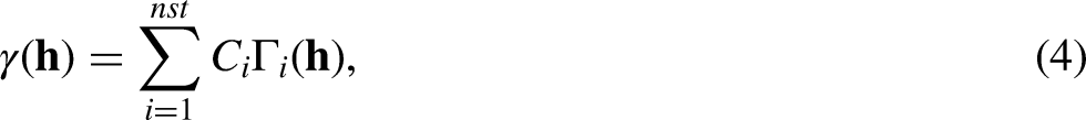
Stochastic modeling methods such as semivariogram-based modeling condition the spatial context of the spatial dataset while integrating domain expertise via the interpretation of spatial, geological concepts such as geometric anisotropy, spatial trend information, spatial continuity, and nugget effect. Assuming stationarity, the experimental semivariogram can be calculated as:

$$\gamma (\mathbf{h})={\displaystyle \frac{1}{2}\mathbb{E}\{{[Z(\mathbf{u}+\mathbf{h})-Z(\mathbf{u})]}^2\},\mathrm{\forall }\mathbf{u},\mathbf{u}+\mathbf{h}\in areaofinterest}$$

(3)

where $\gamma (\mathbf{h})$ is the semivariogram, u is the location vector, h is the lag distance vector connecting all pairs of spatial data locations, $Z(\mathbf{u})$ and $Z(\mathbf{u}+\mathbf{h})$ of Z variable, with the same lag distance and direction (Journel and Huijbregts 1978; Isaaks and Srivastava 1989; Pyrcz and Deutsch 2014). Semivariogram is half of the variogram, $2\gamma (\mathbf{h})$ , but commonly referred to as variogram for short. The variogram model is fitted according to the calculated experimental variogram values and domain knowledge with a permissible, positive definite parametric nested set of variogram structures providing a continuous function that is valid for all lag distances and directions as:

$$\gamma (\mathbf{h})=\sum _{i=1}^{nst}{C}_i{\mathrm{\Gamma }}_i(\mathbf{h}),$$

(4)

where nst is the number of nested variogram structures, $C_i$ is the variance contribution of each nested variogram structure and ${\mathrm{\Gamma }}_i(\mathbf{h})$ is the specific variogram structure for a linear combination of each variance contribution, such as spherical, exponential and Gaussian (Deutsch and Journel 1997). The variogram range a describes the maximum lag distance of correlation to quantify spatial continuity, beyond which there is no correlation between $Z(\mathbf{u})$ and $Z(\mathbf{u}+\mathbf{h})$ . Under the assumption of stationarity, covariance and variogram are equivalent for two-point correlation characterization. The stationary covariance is defined as:

$$C(\mathbf{h})=\mathbb{E}\{Z(\mathbf{u}+\mathbf{h})Z(\mathbf{u})\}-[\mathbb{E}\{Z(\mathbf{u})\}{]}^2,\mathrm{\forall }\mathbf{u},\mathbf{u}+\mathbf{h}\in areaofinterest$$

(5)

where covariance $C(\mathbf{h})$ quantifies the similarity of the random functions, $Z(\mathbf{u})$ and $Z(\mathbf{u}+\mathbf{h})$ , over lag distance $\mathbf{h}$ . Correlogram, $\rho (\mathbf{h})$ , is defined as a normalized covariance:

$$\rho (\mathbf{h})={\displaystyle \frac{C(\mathbf{h})}{C(0)}}$$

(6)

where $C(0)$ is equivalent to the stationary variance, ${\sigma }^2$ . The relation of correlogram, covariance and variogram can be described as:

$$C(\mathbf{h})=\rho (\mathbf{h})\cdot {\sigma }^2={\sigma }^2-\gamma (\mathbf{h})$$

(7)

The correlogram, $\rho (\mathbf{h})$ , is the correlation coefficient of the h-scatter plot at the lag distance h, where the jointly formed random functions $f_{Z(\mathbf{u}),Z(\mathbf{u}+\mathbf{h})}(z(\mathbf{u}),z(\mathbf{u}+\mathbf{h}))$ of the random variables tail, $Z(\mathbf{u}),$ and head, $Z(\mathbf{u}+\mathbf{h})$ , are scatter-plotted.

For variogram-based methods, the impact of scale can be accounted for by adjusting variogram models based on analytical solutions derived from the scaling law indicating how the statistics such as histogram or variogram change with respect to scale (Kupfersberger et al. 1998; Frykman and Deutsch 2002). Denoting a smaller scale of $|v|$ and a larger scale $|V|$ , the variogram model parameters can be updated accordingly assuming the shape of the variogram structure remains the same and the variable scales linearly. For example, the difference in variogram range of a larger scale $a_V$ and a smaller scale $a_v$ is

$$a_V=a_v+(|V|-|v|)$$

(8)

The variance contribution from each nested structure $C_i$ changes by

$$C_{V,i}=C_{v,i}{\displaystyle \frac{1-\overline{\gamma }(V,V)}{1-\overline{\gamma }(v,v)}}$$

(9)

where $\overline{\gamma }$ is the average variogram numerically calculated from the scale where we have the best knowledge of the correlation structure. The variance of the completely random component of the variogram, nugget effect $C^0$ , is inversely related to volume changing ratio, i.e.,

$$C_V^0=C_v^0{\displaystyle \frac{|v|}{|V|}}$$

(10)

Liu and Pyrcz (2021) proposed a spatial anomaly detection method that utilizes correlogram to infer bivariate joint probability distribution for data pairs to calculate the anomaly probability of sparsely sampled spatial data. While Liu and Pyrcz (2021)’s method practically calculates spatial anomaly probability for any pair of sparsely sampled data, it may be redundant and impractical for exhaustively sampled, 2D or 3D regular grid-based datasets, such as satellite images and inverted seismic-derived attributes models. In addition, for an exhaustive dataset, the definition of anomaly can change with respect to the scale of interest, e.g., grid size for a 2D map or cell volume for 3D model, which should be addressed accordingly.

Convolutional neural networks (CNN) integrate spatial neighboring information and are applied to exhaustive gridded data, via training various weighted filters known as kernels that process different features from images (Goodfellow et al. 2016), e.g., auto-encoder, generative adversarial network (GAN, Goodfellow et al. 2014; Schlegl et al. 2017). One example is auto-encoders that consist of the architecture of an encoder and a decoder. The encoder projects the original data into low-dimensional feature space, while the projected low-dimensional space is to be recovered by the decoder. The parameters of the encoder and decoder are learned in the process of optimizing a reconstruction loss function (Hinton and Salakhutdinov 2006; Vincent et al. 2010). Auto-encoders are used for anomaly detection relying on the assumption that non-anomalous observations can be better restructured from the compressed low-dimensional space than anomalies (Pang et al. 2020). However, they are in general treated as a black-box application, with limited interpretability, and can suffer from the limitations of complicated machine learning models requiring a lot of labeled data to train a large amount of model parameters, and the potential for model overfit. To practically identify anomalies in a big, spatial dataset and save professional time, a simple quality control tool with moderate interpretability for domain expertise would be more practical for quick diagnostics.

We propose a novel spatial anomaly detection method for exhaustively mapped data through ensembles of anomaly probabilities within a local neighborhood over the 2D map or 3D model, which is an extension of Liu and Pyrcz (2021) method designed for sparsely sampled spatial data. Our spatial anomaly detection method for exhaustive datasets is simple to calculate and retains flexibility for integrating scale of interest and domain expertise. Ensemble methods are a general meta-approach that uses multiple statistical or machine learning estimators to obtain better predictive performance than could be obtained from any single estimator alone (Opitz and Maclin 1999). The idea of ensemble learning is widely applied in machine learning, such as bagging, stacking, and boosting (James et al. 2013). Some deep learning architectures are also inspired by ensemble learning, e.g., CapsNet (Sabour et al. 2017) which reuses output from a subset of lower level “capsule” structure, i.e., a group of neurons, to form more stable representations against various perturbations for higher-level capsules. The proposed ensemble spatial anomaly detection repeats the pairwise classification locally within a moving search window to formulate an aggregation of classifications (anomaly or not an anomaly) and then identifies spatial anomalies through the majority vote of ensemble anomaly classifiers. The proposed method improves data-driven methods for exhaustive spatial data via the integration of geosciences and engineering expertise with the innovative adaption of variogram-based modeling and finds a robust way accommodating multiple anomaly probabilities for a single location inspired by ensemble learning. In summary, this paper is an extension of the variogram-based spatial anomaly detection method for the case of exhaustive, gridded datasets. We present a novel method that makes it applicable for exhaustive data and with 3 end member cases demonstrate its efficiency in detecting local anomalies as well as transition zone boundaries for different scales.

In the next section, we explain our methodology for anomaly probability calculation, classification and ensemble. In the results section, we show the results and analysis demonstrated with a synthetic acoustic impedance model with the inclusion of data artifacts as well as a mixed spatial population model with transition zones. We show that the proposed method is able to identify spatial population transitions and local artifacts in exhaustive spatial datasets well. Then we conduct a sensitivity analysis on the anomaly detection map with respect to different grid sizes to investigate the impact of scale on the anomaly detection.

Method

Our proposed method for exhaustive mapped data anomaly detection is based on the moving search window of the ensemble of pairwise anomaly probability applied for each grid node, $Z(\mathbf{u})$ , over the adjacent nodes within the moving window, $Z(\mathbf{u}+\mathbf{h})$ . For each pair of neighboring grid nodes, the calculation of anomaly probability is adapted from the spatially-correlated anomaly detection method by Liu and Pyrcz (2021) and is treated as a single classifier in the presence of an anomaly. The anomaly classification is based on a user-pick probability threshold to compare with the measure of probability applied to identify anomalous data pairs. The anomaly state of the current grid node, $Z(\mathbf{u})$ , is decided based on the majority rule of the ensemble anomaly classifiers within the moving search window. Leveraging the idea of ensemble learning, we extend the spatial anomaly detection method for sparse samples to exhaustive datasets.

The flowchart for the proposed spatial ensemble anomaly detection method is demonstrated in Figure 1. The detailed steps are specified as:

Data preprocessing: Model systematic trends of the exhaustively mapped data if present. Conduct a normal score transformation for the exhaustive-mapped data or residuals after trend removal to transform data into standard Gaussian random function Z.

Fit a nested positive-definite variogram model to the directional experimental variograms obtained from the transformed data integrating analog information and domain expertise.

For location ${\mathbf{u}}_i,i=1,2,\dots ,n$ , where n is the number of grid nodes of the mapped data:

For lag distance ${\mathbf{h}}_j,j=1,2,\dots ,m$ where m is the number of neighboring node locations, ${\mathbf{u}}_i+{\mathbf{h}}_j$ , within the moving search window given the current grid node location ${\mathbf{u}}_i$ :

Calculate correlogram $\rho ({\mathbf{h}}_j)$ from variogram value $\gamma ({\mathbf{h}}_j)$ at the given lag distance ${\mathbf{h}}_j$ based on Eq. 7.

Infer the joint bivariate probability density space for the random variable of grid node $Z({\mathbf{u}}_i)$ and the random variable of adjacent node $Z({\mathbf{u}}_i+{\mathbf{h}}_j)$ based on the corresponding stationary correlogram $\rho ({\mathbf{h}}_j)$ assuming a bivariate Gaussian distribution:

$$f_{Z({\mathbf{u}}_i),Z({\mathbf{u}}_i+{\mathbf{h}}_j)}(z({\mathbf{u}}_i),z({\mathbf{u}}_i+{\mathbf{h}}_j))={\displaystyle \frac{1}{2\pi {\sigma }^2{\sqrt{1-\rho ({\mathbf{h}}_j)}}^2}\exp \left[-{\displaystyle \frac{b}{2(1-\rho {({\mathbf{h}}_j)}^2)}}\right]}$$

(11)

where b is expressed as

$$b={\displaystyle \frac{{(z({\mathbf{u}}_{\mathrm{i}})-\mu )}^2-2\rho (z({\mathbf{u}}_{\mathrm{i}})-\mu )(z({\mathbf{u}}_i+{\mathbf{h}}_j)-\mu )+{(z({\mathbf{u}}_i+{\mathbf{h}}_j)-\mu )}^2}{{\sigma }^2}}$$

(12)

$\mu$ , ${\sigma }^2$ is the stationary mean and variance, respectively.

Discretize the joint probability density space into meshed grids made up of $\mathrm{\Delta }Z({\mathbf{u}}_i)$ , $\mathrm{\Delta }Z({\mathbf{u}}_i+{\mathbf{h}}_j)$ . Determine the joint probability density of each grid based on the joint probability density function $f_{Z({\mathbf{u}}_i),Z({\mathbf{u}}_i+{\mathbf{h}}_j)}(z({\mathbf{u}}_i),z({\mathbf{u}}_i+{\mathbf{h}}_j))$ in Eq. 11 given the corresponding correlogram $\rho ({\mathbf{h}}_j)$ between the given pair of grid nodes $z({\mathbf{u}}_i)$ and $z({\mathbf{u}}_i+{\mathbf{h}}_j)$ .

Normalize the joint probability density of each grid to ensure the closure, i.e., probability of each grid sum up to 1, is satisfied over the discretized joint probability density function in Eq. 13.

$$\underset{-\mathrm{\infty }}{\overset{+\mathrm{\infty }}{\int }}\underset{-\mathrm{\infty }}{\overset{+\mathrm{\infty }}{\int }}{f}_{Z({\mathbf{u}}_i),Z({\mathbf{u}}_i+{\mathbf{h}}_j)}(z({\mathbf{u}}_i),z({\mathbf{u}}_i+{\mathbf{h}}_j))dZ({\mathbf{u}}_i)dZ({\mathbf{u}}_i+{\mathbf{h}}_j)=1.0$$

(13)

Calculate joint cumulative probability by summing up the joint probability of each grid in a descending manner until finding the grid where the given pair of grid nodes, $z({\mathbf{u}}_i)$ and $z({\mathbf{u}}_i+{\mathbf{h}}_j)$ locates.

Calculate the complement of joint cumulative probability that is later utilized as anomaly probability for each classifier. The anomaly probability describes the probability of a less likely combination, $z({\mathbf{u}}_i)$ and $z({\mathbf{u}}_i+{\mathbf{h}}_j)$ , in the complete joint probability space quantifying the anomalous degree of the observed grid nodes combination.

Assign the ensemble anomaly classifier of the current pair of nodes based on the anomaly probability and user-pick probability cutoff.

Aggregate all the m anomaly classifiers for the current grid node within the current searching window by majority vote, i.e., the current node is an anomaly if the majority of the classifiers are anomalous.

Figure 1.

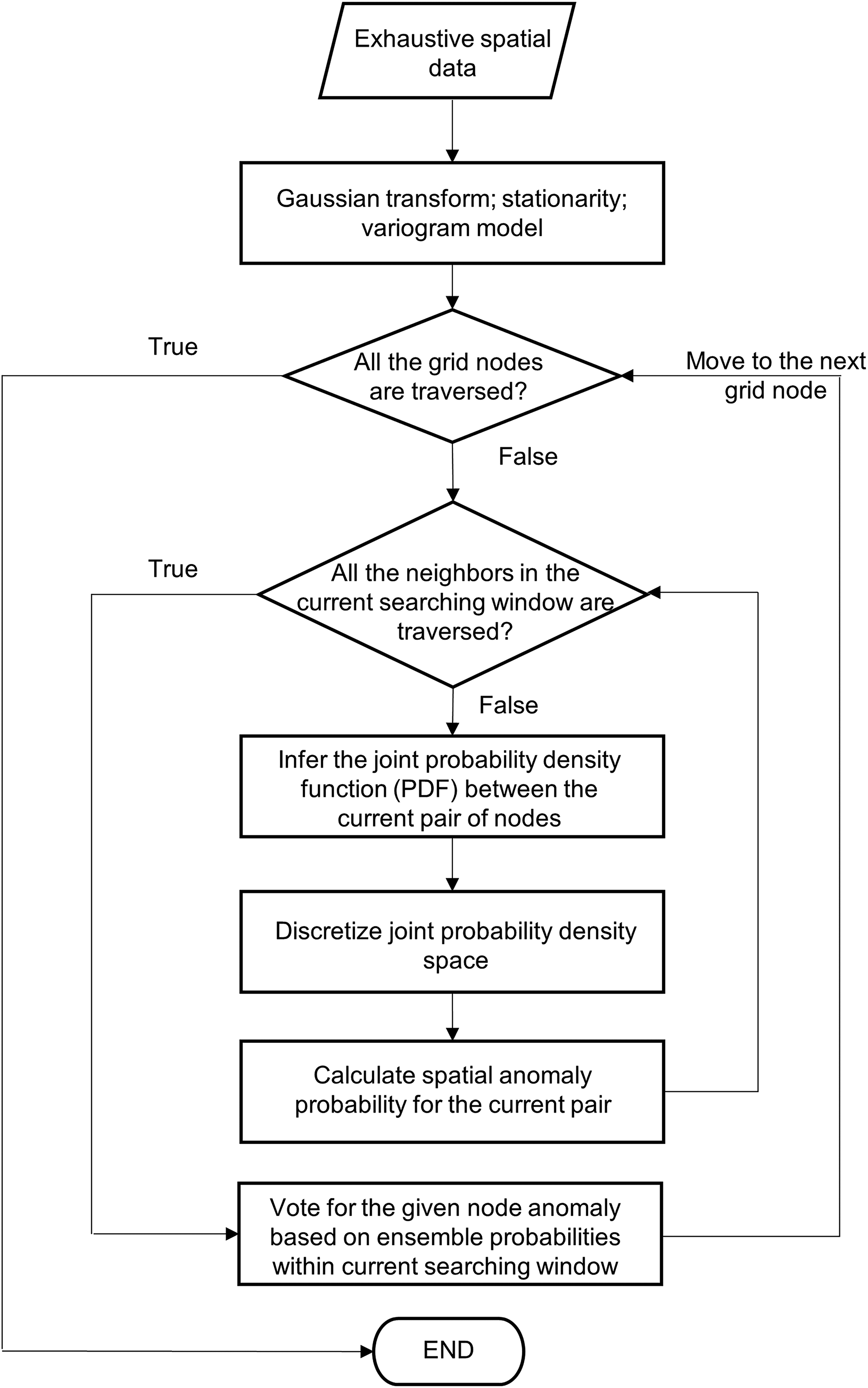
Ensemble spatial anomaly detection method flow chart.

According to the proposed method, there are two potential hyperparameters that may impact the results. One is the anomaly probability cutoff when deciding if a pair is anomalous or not. The other one is the size of the moving search window, i.e., the maximum range for a grid to construct a pair for calculating anomaly probability, as the spatial correlation is getting weaker as the lag distance of a pair gets further. The anomaly probability cutoff is up to the user based on the cost of risk in practice, i.e., the preference for over-estimation or under-estimation. We conduct a sensitivity analysis to evaluate the impact of the size of the moving window and discuss the impact in the results section.

Results

We demonstrate the proposed method with several synthetic datasets that mimic the possible spatial use cases and data issues. First, we construct a synthetic 2D acoustic impedance model from sequential Gaussian simulation (SGSim) and a non-linear affine transformation (Pyrcz et al. 2021). Secondly, we add data artifacts as hot pixel in case 1 and compare the spatial anomalies detected by the proposed method with univariate anomalies identified based on global distribution. Then, we construct a two facies porosity model to represent a mixed population model in case 2 and find the proposed method can effectively identify the transition zone boundary. Lastly, for the facies model in case 2, we inspect the anomaly detection results adjusted for different scales. We find that, as the scale goes from fine-scale to coarse-scale, the anomalies detected evolve from boundaries to clusters.

The visualization of the acoustic impedance model and the corresponding histogram is shown in Figure 2 and the variogram model parameters are given in Table 1. A sensitivity analysis for the hyperparameter, the size of the moving window, is demonstrated with the acoustic impedance model. When the window size is significantly larger than the spatial continuity range, pairs with no spatial correlation dominate the votes and anomalies identified by the spatial method may converge to the results from the univariate method. Therefore, an appropriate window size is constrained by the range of spatial continuity and the scale of the area of interest In this demonstration, the spatial continuity range is much larger than the window size as shown in the parameters in Table 1, which justifies the use of our spatial anomaly detection method. We conduct the sensitivity analysis where the moving window size varies from 1 unit lag distance to 18 unit lag distance and the results are shown in Figure 3. We employ the proportion of anomalies identified by the detection method with respect to the total number of pixels as a simple metric to evaluate the sensitivity. We choose anomaly probability cutoff as 5% by default as it is a commonly chosen cutoff for univariate anomaly detection, i.e., we expect to cut off 5% of the total number of pixels as anomalies. So the window size that yields 5% spatial anomalies with respect to the total number of pixels is the appropriate size for the case, namely, 7 unit lag distance, and we will use the results from this window size for the rest of the analysis in this section.

Figure 2.

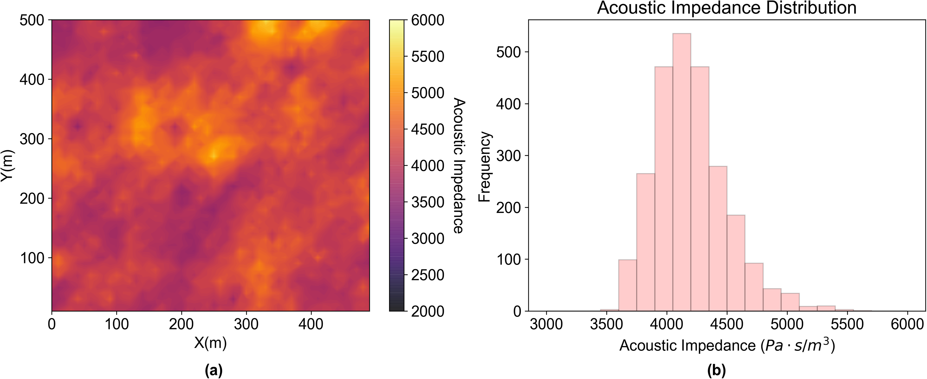
(a) Acoustic impedance model (b) the histogram of acoustic impedance model.

Figure 3.

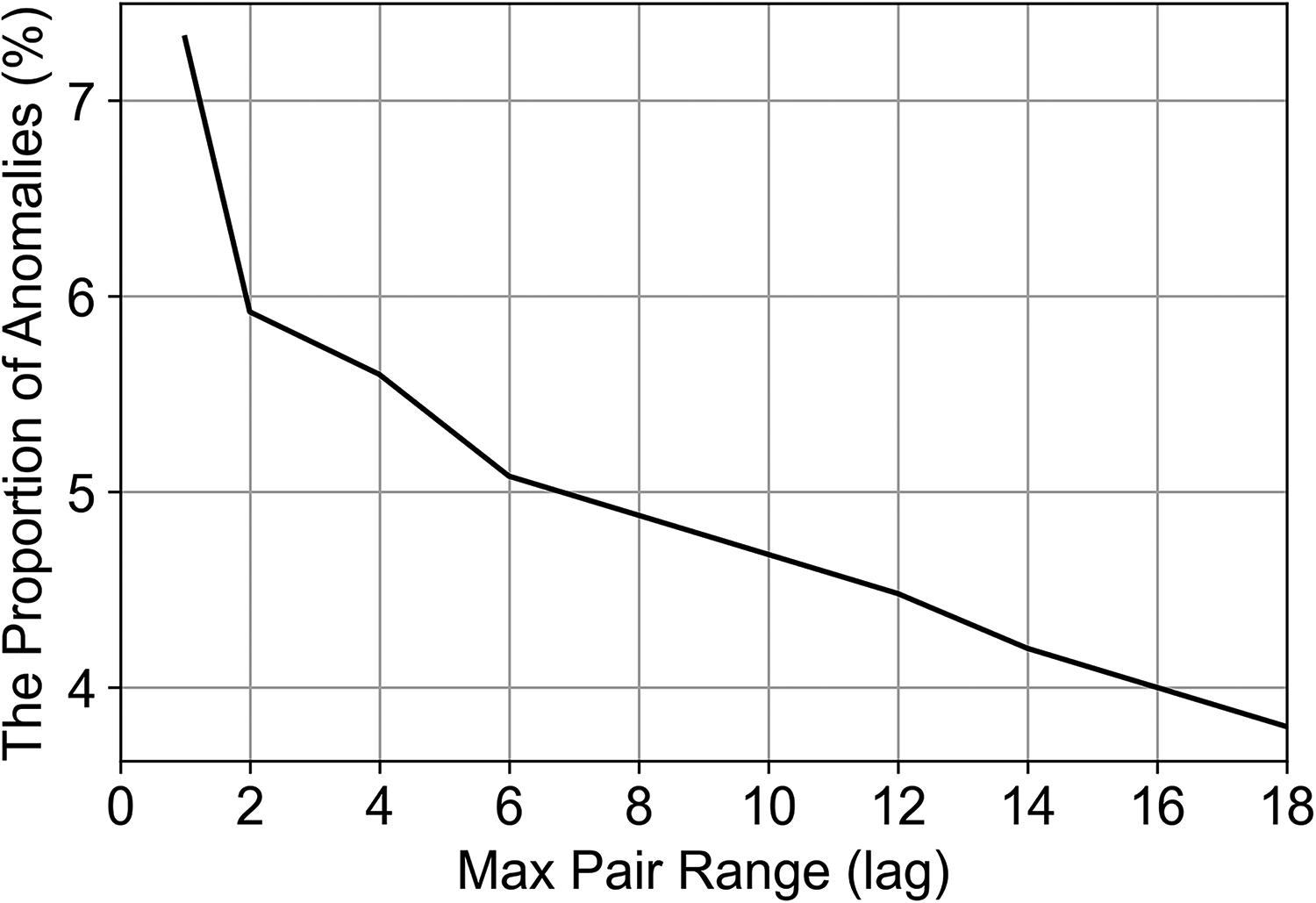
Proportion of anomalies with respect to the total number of pixels with majority vote for each grid node vs. moving window size (lag) for a grid to construct a pair for calculating anomaly probability.

Table 1.

Variogram model parameters.

Nugget Effect = 0	Azimuth = 30	Grid (lag) size = 10 (m)
Variogram structure type	Major direction range (m)	Minor direction range (m)
Spherical	500	300

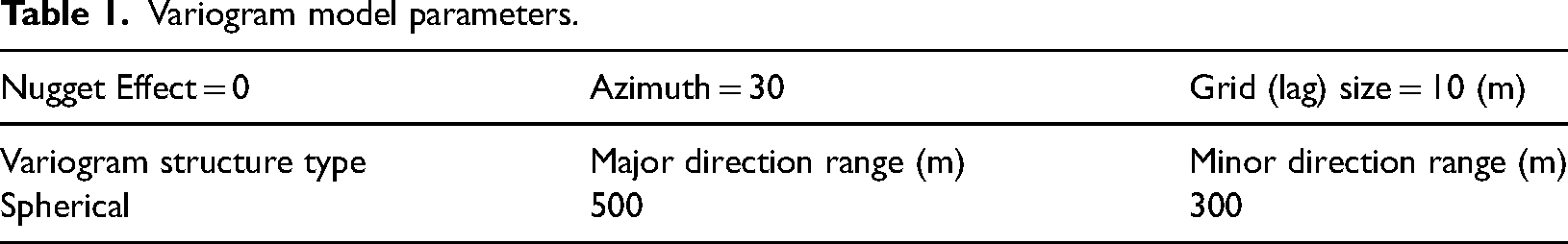
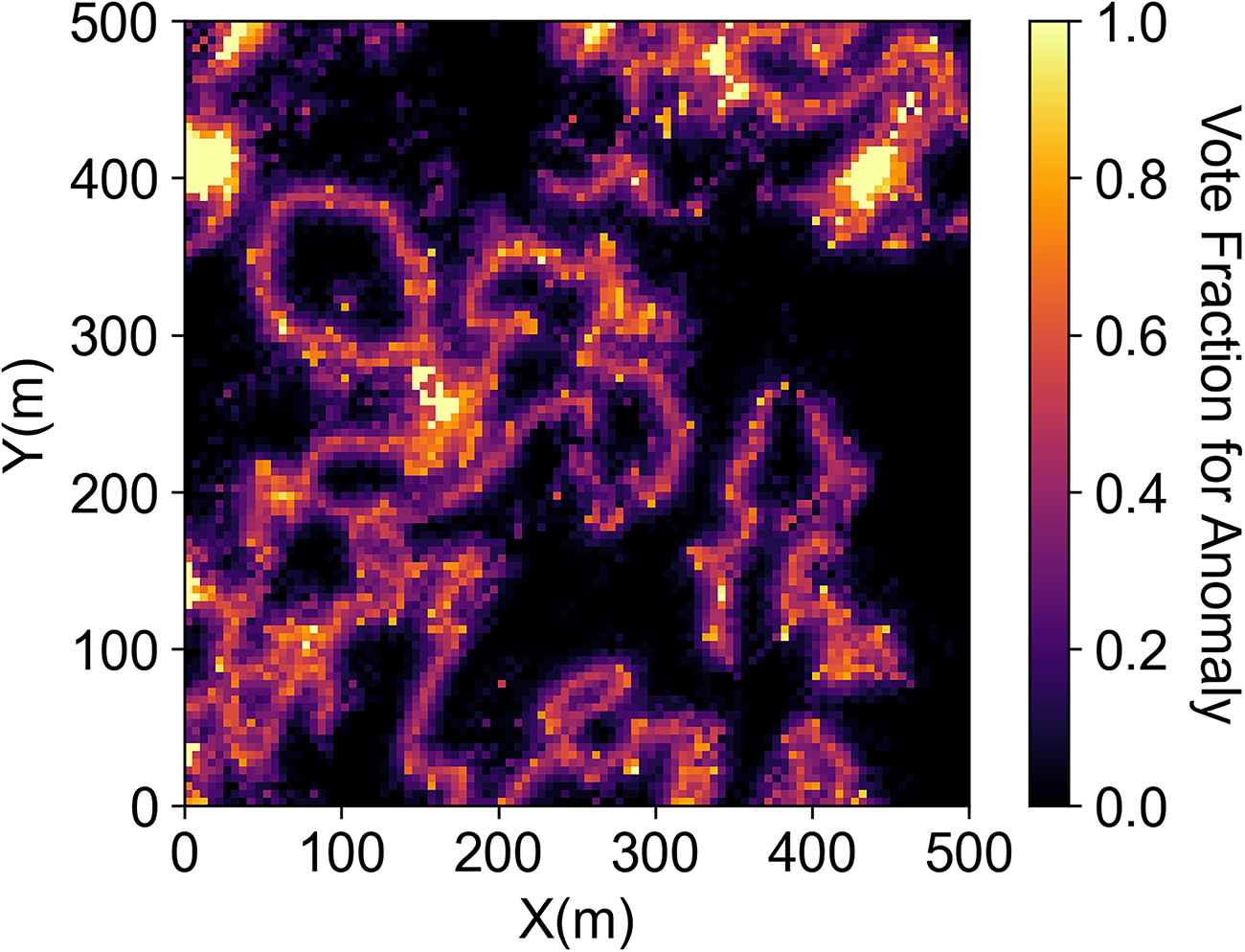
 Figure 4 shows the ensemble proportion map of votes for anomaly of each grid node, a measure of anomaly uncertainty. Figure 5 shows the location of the anomalous regions based on the majority rule of the vote from the ensemble spatial anomaly detection when moving window size is tuned to provide 5% anomalies of the total number of pixels compared with the univariate anomalies based on the 5% two-tail of the global distribution. For the same proportion of spatial anomalies, univariate anomaly detection only finds the global extreme values while the spatial anomaly detection identifies some global anomalous regions as well as local anomalies due to the random sampling and random path of sequential Gaussian simulation.

Figure 4.

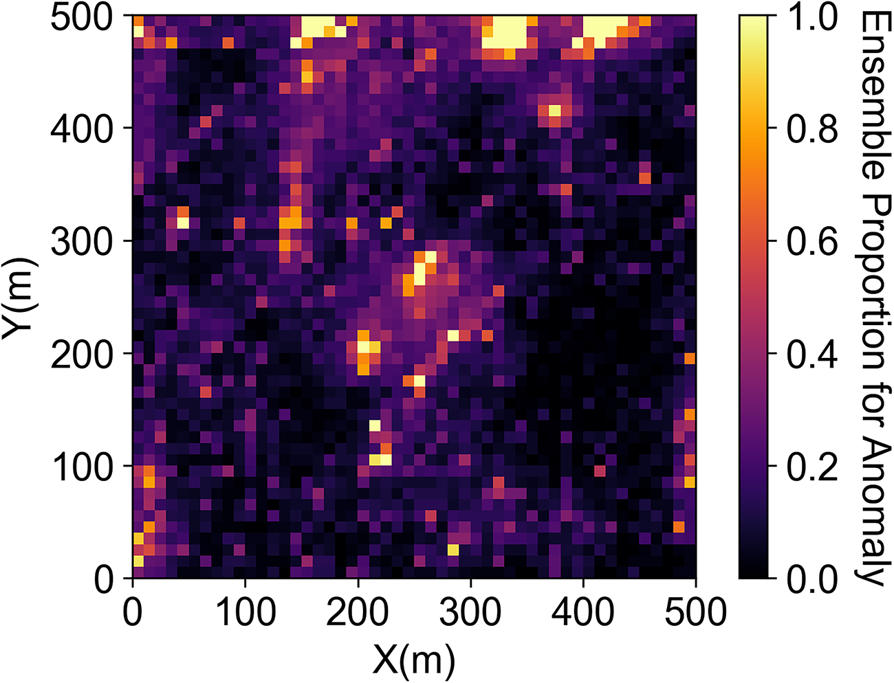
Ensemble proportion classification map of anomaly.

Figure 5.

(a) Anomaly map based on spatial anomalies (orange) and univariate anomalies (purple) and their overlap (ivory) for 5% anomalies (b) anomalies (5%, white scatter) identified by spatial anomaly detection method (c) anomalies (5%, white scatter) identified by univariate anomaly detection.

Case 1: hot pixel

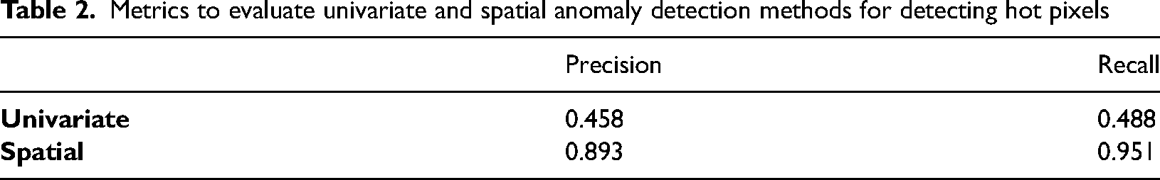
For case 1, we swap grid nodes to introduce 5% hot pixel artifacts to the original acoustic impedance model, while not changing the global distribution, to mimic the hot pixels that commonly happen in exhaustive mapped data. The visualization of the dataset and the corresponding histogram are shown in Figure 6. Figure 7 shows the ensemble proportion for each pixel being an anomaly. We find the hot pixels are categorized as anomalies with an ensemble proportion close to 1, which indicates the proposed method can identify data artifacts with high confidence. We assess the difference between the spatial anomalies detected by our proposed method and the extreme values at the tail of the global distribution, i.e., univariate anomalies, in Figure 8. Given the constraint of the same proportion of anomalies in Figure 8(b) and (c), the proposed method can detect the hot pixel locations with better precision and recall than the univariate anomalies according to the metrics in Table 2 as well as visual inspection. Due to the data imbalance, i.e., there are a lot more normal data than anomalies, accuracy is not a good metric for evaluation.

Figure 6.

(a) Acoustic impedance model with 5% hot pixels (b) the histogram of acoustic impedance with hot pixels.

Figure 7.

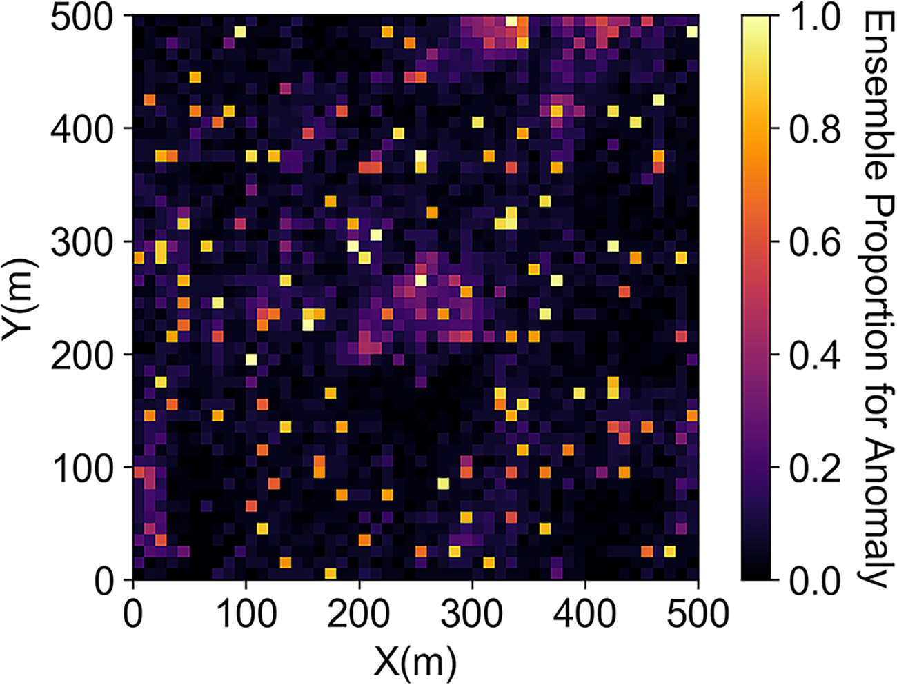
Ensemble proportion classification map for acoustic impedance model with hot pixels.

Figure 8.

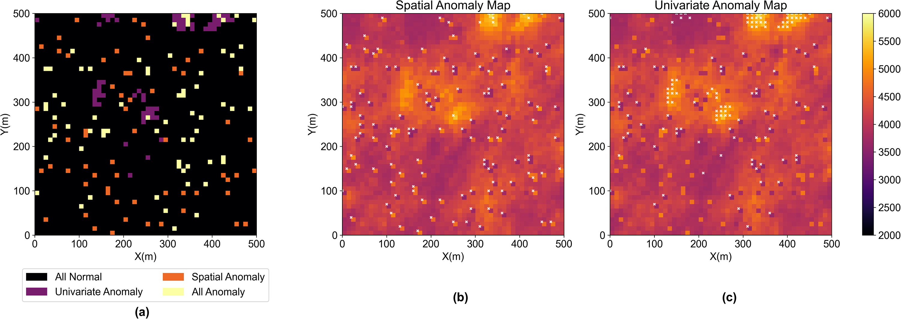
(a) Anomaly map based on spatial anomalies (orange) and univariate anomalies (purple) and their overlap (ivory) for identifying hot pixels (b) anomalies (white scatter) identified by spatial anomaly detection method (c) anomalies (white scatter) identified by univariate anomaly detection.

Table 2.

Metrics to evaluate univariate and spatial anomaly detection methods for detecting hot pixels

	Precision	Recall
Univariate	0.458	0.488
Spatial	0.893	0.951

Case 2: facies boundary

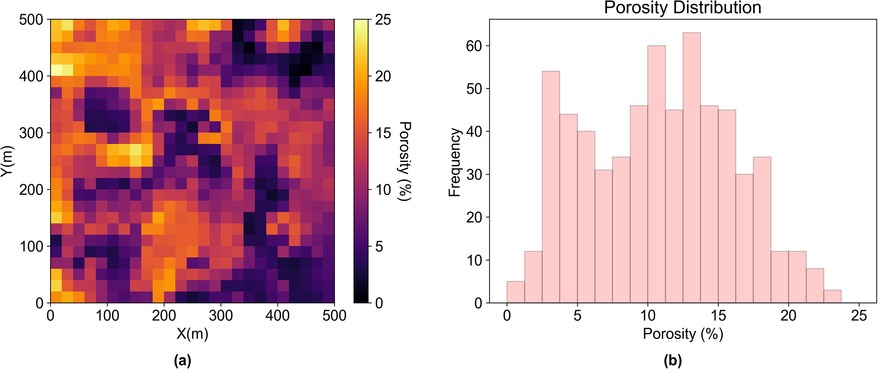
For case 2, we build a two-facies porosity model with bimodal global distribution. The distinct facies boundaries and the bimodal histogram are visualized in Figure 9. The grid nodes on the map in Figure 10 with high ensemble proportion clearly indicate the transition zone boundary. There are some clusters on the map with an ensemble proportion close to 1. We compare the results from the proposed method and univariate anomaly in Figure 11. We find the clusters with high ensemble proportion in Figure 11 are the overlapping regions between the proposed method and univariate anomaly, which are only the global extreme values.

Figure 9.

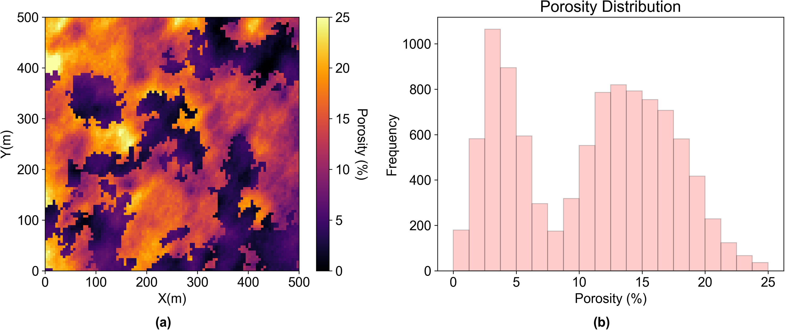
(a) Porosity model with two facies (b) the histogram of the bimodal porosity model.

Figure 10.

Ensemble proportion classification map for transition zone boundary uncertainty.

Figure 11.

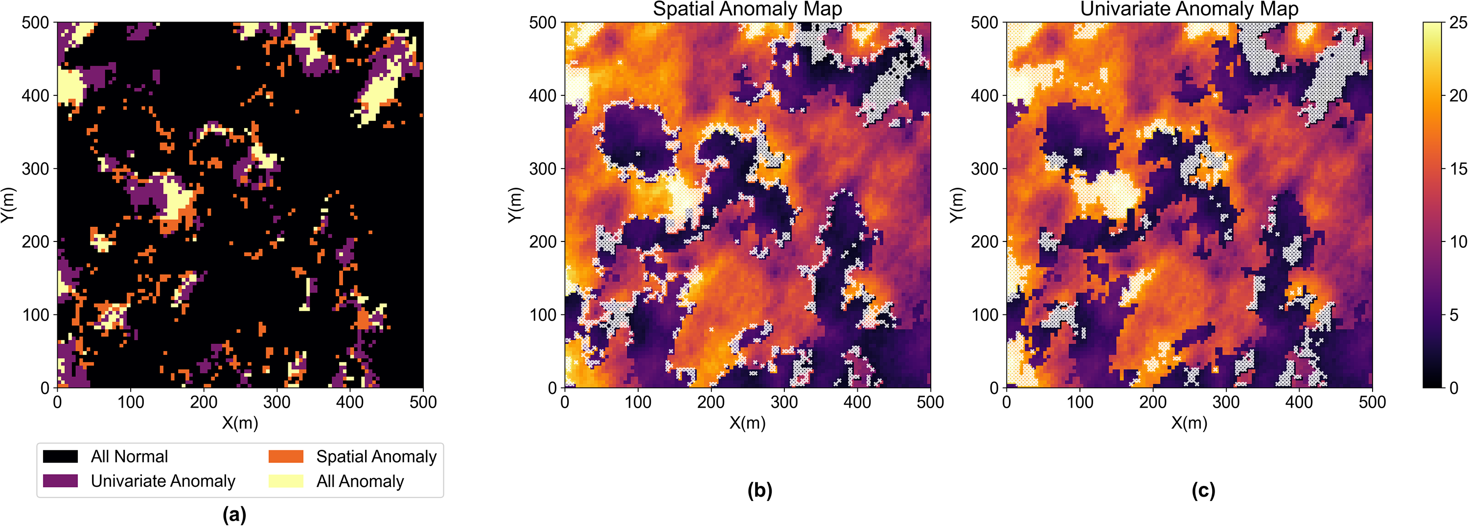
(a) Anomaly map based on spatial anomalies (orange) and univariate anomalies (purple) and their overlap (ivory) for transition zone boundary (b) anomalies (white scatter) identified by spatial anomaly detection method (c) anomalies (white scatter) identified by univariate anomaly detection.

Case 3: sensitivity analysis of scale

The area of interest in case 2 is modeled by 100 $\times$ 100 grids with cell size 5 m in both X and Y directions. For the sensitivity analysis of scale, we rescale the model for the same area of interest from a fine-scale 100 $\times$ 100 model to a coarser scale 50 $\times$ 50 and 25 $\times$ 25 with corresponding grid size, 10 m and 20 m with the assumption of linear averaging The rescaled models are shown in Figure 12 and Figure 13. After rescaling, the distinct facies boundaries are smoothed out and variability decreases. Our spatial anomaly detection method robustly applies the volume variance scaling law to correct the variogram and histogram for the change in scale. The spatial anomalies from fine and coarse scales are superimposed in Figure 14. Since the transition zone boundary is smoother as cell size increases, the spatial anomaly detection method picks up larger scale transitions and average boundaries.

Figure 12.

(a) Rescaled 50 $\times$ 50 porosity model (b) the histogram of the corresponding rescaled model.

Figure 13.

(a) Rescaled 25 $\times$ 25 porosity model (b) the histogram of the corresponding rescaled model.

Figure 14.

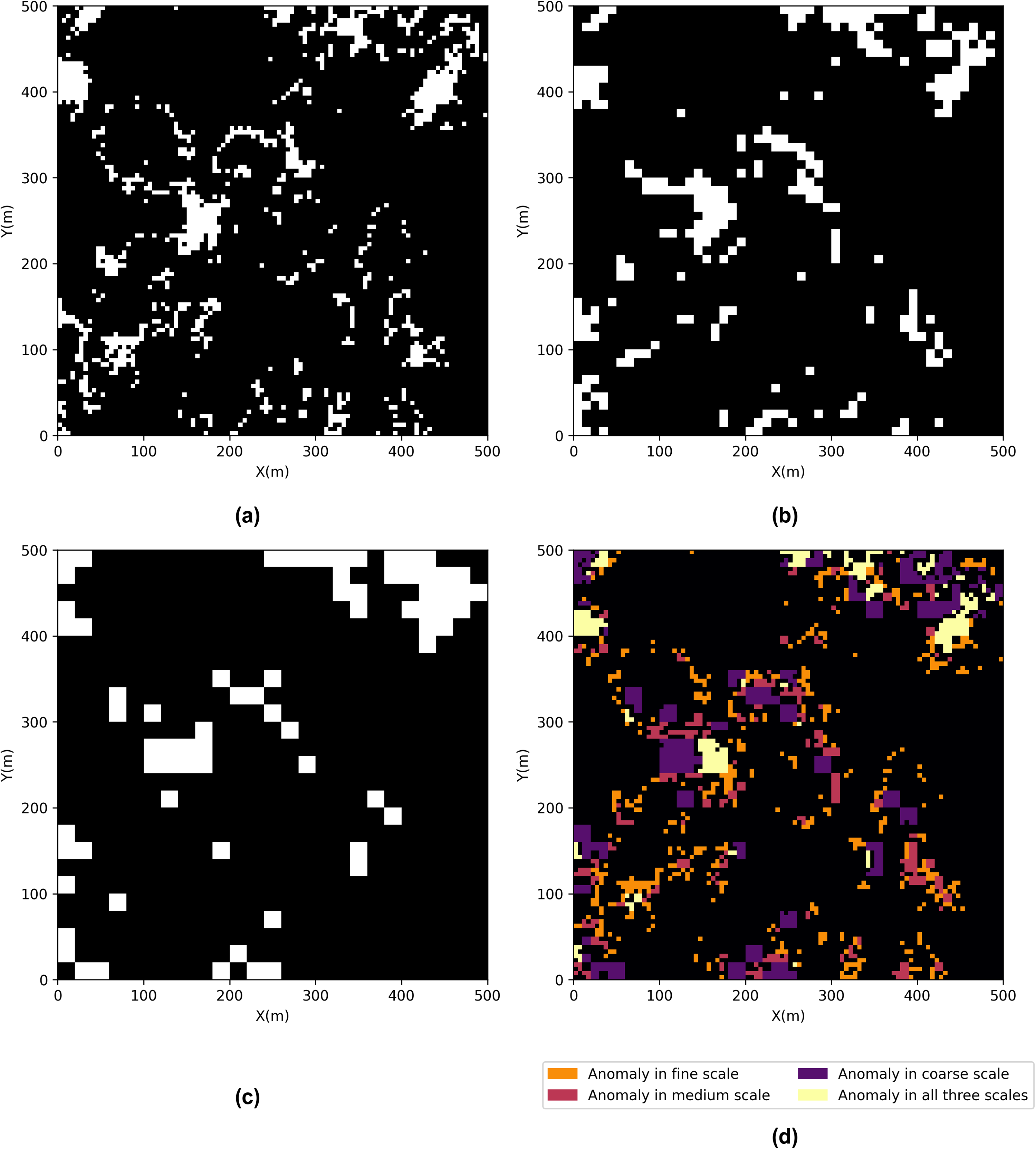
(a) Spatial anomalies of fine-scale (100 $\times$ 100) (b) spatial anomalies of medium-scale (50 $\times$ 50) (c) spatial anomalies of coarse-scale (25 $\times$ 25) (d) spatial anomalies superimposition of fine-scale, medium scale, and coarse-scale.

Conclusion

We propose an ensemble spatial anomaly detection method for exhaustively sampled data, e.g., 2D geological maps and seismic sections or 3D subsurface models and seismic attributes, to help identify spatially anomalous regions and transition zone boundaries for the different scales while remaining interpretable for domain knowledge through variogram modeling and trend modeling. Due to the spatial correlation among spatial data, the moving window size can be treated as a hyperparameter for the proposed method to tune to obtain a reasonable number of anomalies or a clear boundary line. We demonstrate the proposed method can effectively identify hot pixels in the image as well as mixed population transition zone boundaries. The proposed method is responsive to the spatial local anomaly and distinct boundary transition while the univariate anomalies extracted from global distribution ignore spatial context. We suggest utilizing the proposed spatially aware detection method to automate the local anomaly and boundary identification process.