Sage Journals: Discover world-class research

Abstract

Manual evaluation of military target camouflage often fails to fully capture human visual characteristics. This paper introduces a method for intelligent camouflage feature extraction and effect evaluation using deep neural networks. Firstly, military target and background datasets are constructed, with annotation methods optimized through perceptual experiments. A GANomaly model for background anomaly detection and a transfer learning feature model are developed. These models evaluate data similarity to background and target features to categorize camouflage into three levels. PCA dimensionality reduction and RFE screening identify final features. Two logistic regression models are then combined to create a grading model. In experiments, the GANomaly model was trained and optimized, achieving 86.8% accuracy in distinguishing level 1 from non-level 1 camouflage using 28-dimensional features. Among three transfer models, the MobileNetV2 model identified 33-dimensional features with 85.1% accuracy in distinguishing level 3 from non-level 3 camouflage. Combined, the models reached an 84.3% grading accuracy on the test set, with Micro and Macro average AUC values of 0.939 and 0.945, respectively. This performance surpasses that of BP network models and linear models based on manual features, as well as metrics like SSIM, UIQI, MSE, and PSNR. The results indicate that the models effectively align with human annotations and can reliably assess military target camouflage levels.

Keywords

Camouflage evaluation visual features deep learning anomaly detection

Introduction

Camouflage effect evaluation of military targets plays a very important role in combat training applications.¹ At present, most of the camouflage materials in military equipment are composed of textiles. Good camouflage effect evaluation can promote the optimization and upgrading of military textile equipment pattern design. Camouflage effect evaluation and modeling is mainly aimed to simulate the process in which human observers discover and understand a target, and then conclude the significance of a target in the background where it is located.^2,3 However, when human observe a target, many factors are involved, including target factors, and the differences between individual features.^4,5 The target factor refers to different targets having different perspectives, different forms of target factors, and different features and textures presented by different targets. Individual characteristics refer to the varying levels of mastery of military knowledge among individuals, as well as the different scales of target grasping, resulting in different judgments. These factors influence the complexity and difficulty of the evaluation and modeling of camouflage effect.⁶

Currently, the main mode of the existing theoretical model is as follows. Evaluation results were formed by constructing the feature index system of a target and its combination algorithm, and the results were mostly expressed by discovery probability or feature similarity. Many scholars^7–9 have done a lot of research from the two aspects of “indicator system” and “feature combination”. In terms of feature extraction, Ajoy Mondal et al.¹⁰ divided the existing camouflage effect evaluation models into four types, including (I) salience models, (II) global cluster metric, (III) local cluster metric, and (IV) other technologies. They affirmed the important role of military target benchmark data set, and proposed that deep learning model is the future development trend of camouflage design evaluation. At the same time, they also discussed the advantages and feasibility of semi-supervised learning and unsupervised learning under a small number of marked military target samples. Timothy et al.¹¹ modeled low-level visual processing (log Gabors), and evaluated the significance of military helmets in different countries by estimating the parameters of multivariate gaussian mixture distribution. By extracting a gray-level co-occurrence matrix of local binary pattern (LBP) images, Jian Chaochao et al.¹² obtained five features describing the texture features of images to achieve the illumination invariance of them. Bai et al.¹³ proposed the Image Color Similarity Index (ICSI) and Gradient Similarity Difference (GMSD) to analyze the color and texture differences of background and camouflage images, respectively. Gan et al.¹⁴ proposed the evaluation model of motion camouflage effect based on brightness (L), hue (C), texture (T), shape (S), and patch (D) image features. Yogi et al.¹⁵ evaluated Chinese military camouflage pattern based on the Camouflage Similarity Index (CSI). In terms of feature combination, Yu Songlin et al.¹⁶ established an optical image similarity evaluation method based on multi-feature statistics by combining with grayscale, chromaticity and texture features. Ying Jiaju et al.¹⁷ adopted an algorithm in which feature weight was allocated on the basis of the information entropy of the camouflage images’ feature sequence data to establish a model for comprehensive evaluation. Li Jiakun et al.¹⁸ used the Schmidt orthogonal Martin system to calculate the weights of indicators, and then established an evaluation model based on set pair analysis. Yu Jin et al.¹⁹ established a camouflage effect evaluation model by inputting different features into a BP neural network.

A lot of work has been done so far, there are still some limitations. First, the traditional evaluation method only takes feature differences between the target and background as a criterion, but interpreters apply a large amount of prior knowledge in the interpretation of real targets, which will cause that the judgment results of some objects with visual camouflage effect and also with feature differences from the background by the evaluation model is inconsistent with the reality. Second, only the low-level visual features, such as texture, color, brightness, etc., are considered in the extraction of target features. Feature extraction during object interpretation is from the low-level to the high-level.²⁰ However, it is difficult to directly obtain advanced visual features through analytical methods, like extracting the features such as the metallic gloss of targets, and gun barrel contours. Third, brain nerves process the relationship between lots of features at different levels based on complex nonlinear relationship instead of the simple linear combination found in most of existing models.^3,21

Deep neural network models can automatically extract high-dimensional deep visual features and fit complex functions.²² This study proposes a model for evaluating the camouflage effect of images. Firstly, a camouflage target dataset was constructed based on perception experiments, and a method for manually dividing camouflage levels was proposed. Secondly, based on this dataset, a camouflage effect evaluation architecture model Gan Tran is constructed. The model uses the Ganormaly model to detect the similarity between data and background images, and uses the MobileNetV2 model to determine whether the detected features are similar to the target data features, thereby determining the camouflage level. Finally, the final features are determined through PCA dimensionality reduction and RFE screening, and the final classification results are obtained based on a logistic regression model. The experimental results show that the effectiveness evaluation model proposed in this paper has good reliability and stability. This model can be applied to the evaluation and grading of optical camouflage effects for national defense engineering and various textile camouflage patterns.

Construction of camouflage evaluation datasets

Collection of datasets

In the construction of background and target datasets, the background data was acquired by aerial imaging of unmanned aerial vehicles. The drone model is “DJI MAVIC 2 ENTERPRISE”. The ground resolution of control images was about 10 cm, and their pixel size was 112 × 112. The dataset covers forest, grassland, and desert backgrounds from different time periods and regions, with a total of over 28,000 sets of image data. Figure 1 shows the different types of background data in the dataset.

Figure 1.

Three types of background samples in the background dataset.

The construction of models by deep learning methods requires a large number of target datasets as support, but it is difficult to obtain target sets able to fully reflect data distribution due to the confidentiality and particularity of military targets. In this paper, a dataset of military targets with different camouflage measures was collected, covering screen camouflage, equipment coating camouflage, vegetation camouflage, and convenient camouflage.^23,24 The backgrounds in which the targets were located covers all types in the above background set. Since static targets were only highly corrected with the surrounding background, the data of background images 9 times larger than the target size was selected, with the target in the center.²⁵ The sizes of all images were set to 112 $\times$ 112 to facilitate training. The target set contains ground and aerial images from various angles, with over 600 datasets. Moreover, in the process of model training, random horizontal and vertical flips and small-scale affine transformations were carried out the images in the target dataset to compensate for the problem that the dataset was small. Gaussian noise²⁶ was applied to the brightness of the images to simulate all kinds of weather and lighting conditions during imaging.

Rating of the camouflage effects of manually annotated targets

The indicator of discovery probability used in the past has big shortcomings in practice.^27,28 First, an experiment has a high cost. It takes a large amount of manpower and time to arrange a target experiment on discovery probability for one scenario, but a target dataset in general needs to cover multiple scenarios.^29,30 Second, the accuracy of the experiment is greatly influenced by environmental factors. In the same scenario, small differences in experimental setup (such as direction, weather, viewing angle, etc.) may lead to large differences in the evaluation results. Third, parameters have narrow effective windows. Since the discovery probability based on most data settings is 100% or 0, it takes more time to search for effective parameters before setting experimental parameters. Therefore, the following rating method is adopted in this paper.

The first thing drawing an observer’s attention during the observation of targets is the differences between the targets and background, and the prior knowledge of the observer is not necessary at this time.³¹ However, the features extracted are not limited to low-level human visual features such as colors, texture and shapes. For positions with large differences in features, the observer will identify the features of the targets again according to prior knowledge, and then judge the target types. If it is found that the target features are highly matched with the prior knowledge, whether the area contains military targets shall be determined according to the sensory intensities. The following three basic criteria for camouflage evaluation were established in accordance with the above process (Figure 2). One target with small difference from the background can be determined as the level 1 camouflage, otherwise it is necessary to judge its matching degree with the target features in the prior knowledge base. The camouflage effect is deemed as poor if the match is good, so the target is determined as the level 3 camouflage, otherwise it is determined as the level 2 camouflage.

Figure 2.

Flowchart of the evaluation architecture.

A perceptual grouping experiment method was used, which means that an observer observes all the data at once. The observer should understand the above-mentioned grading ideas and task requirements before observation, and then give the classification results according to intuitive feelings. The experiment has no time and environment limits, so the observer can zoom in or out images arbitrarily and observe them repeatedly. This method has advantages of simple experimental setting, simple procedure and easy understanding, and researchers can observe all the data at one time, which greatly reduces the time for observing large-scale datasets. In addition, datasets can be expanded quickly. The disadvantage is that the final results of the probability indicator are found to be continuous interval values, while only discrete camouflage levels can be obtained by the perceptual grouping method.

The experimental process is as follows: there are a total of 50 participants with military objectives and basic knowledge of camouflage design, aged from 28 to 50 years old. By covering participants of different age groups and experiences, the effectiveness of camouflage level classification can be more accurately reflected. Among them, there are 15 soldiers of various grades aged 18 to 24, 20 soldiers aged 24 to 31, and 15 experienced officers and cadres aged 31 to 50. All them had normal or corrected-to-normal vision. The experimental task told to the participants was to classify images into three camouflage levels according to camouflage effect they presented. The experimental data were all placed in a computer folder. The participants copied and pasted them into the folders for the images of the three levels after viewing their content. The observers can freely zoom in or out the images in the process, so as to ensure that the images can actually reach resolution limit that they can distinguish. In addition, the time was not limited in the experiment process, so that the observers can freely change the classified data until they are fully satisfied.

Based on the conclusion of the classification results, a level confirmed by more than half of the participants is determined as the final camouflage level of a target. The camouflage level would not be set up for the dataset with deep divide and without more than half of the target data of the same level. After the experiment, 40.5% of the dataset was classified as the level 1 camouflage, 34.7% as the level 2 camouflage and 24.8% as the level 3 camouflage.

Modeling of camouflage evaluation based on deep visual features

A deep learning model was used to implement the above evaluation criteria. Two groups of models were constructed to distinguish the camouflages of levels 1 and 2 as well as levels 2 and 3. In Model 1, the GANomaly³² deep adversarial network was used to learn the feature distribution of the background dataset, thereby forming anomalous features to distinguish the level 1 camouflage. In Model 2, target transfer features were extracted by the ILSVRC³³ (ImageNet Large-Scale Visual Recognition Challenge) pre-trained model to distinguish the level 3 camouflages. On this basis, a Gan-Trans model was established according to the logistic regression algorithm, and finally the consistency with the evaluation results in the target datasets was achieved through training.

Extract of background differential features

The GANomaly is used to discriminate non-background sample data after learning a large number of background sample features. The architecture consists of two encoder networks, one decoder network, and one discriminator network (Figure 3). The encoder $G_{E 1}$ transforms the input image $x$ to the latent variable feature $z$ , and the decoder $G_{D}$ transforms the latent variable $z$ to the data distribution x′. The $G_{E 1}$ and $G_{D}$ networks constitute the traditional autoencoder network model. The discriminator network $D$ discriminates between the real data $x$ and the generated data x′ to optimize the feature extraction and original distribution restoration ability of the encoder-decoder’s structure. Unlike the traditional adversarial autoencoder network, this model adds an encoder $G_{E 2}$ after the decoder $D$ . After overall training, this structure can reduce the structural stability of the autoencoder network on the one hand and transfer the reasoning process to the latent variable layer on the other, thus reducing the influence of noise.

Figure 3.

Overall structure of the GANomaly model.

The network structure is designed mainly by the convolution layer/deconvolution layer, batch normalization layer, and rectified linear unit layer (LeakyRELU). The convolutional layer/deconvolutional layer is used for feature extraction layer-by-layer; the rectified linear unit layer offers nonlinear activation, so that the function cluster provided by the model structure approximates the real distribution function of the data; the batch normalization layer is used to speed up model convergence. The convolutional/deconvolutional layer, batch normalization layer and activation layer were simply stacked to form a basic structural unit (Figure 4(a)). The encoder and decoder were constructed with the unit respectively (Figure 4(b)), in which the decoder was composed of four layers of basic units. The number of convolution kernels in the latter layer was set to be twice that of the first two layers, and the number in the first layer was set to 32. The size of the kernel was 4 × 4.0 was padded to keep the size after convolution the same as before or 0.5 times the original. LeakyRELU was adopted as the activation function. The encoder finally output 128-dimensional features. The decoder and encoder are almost completely axisymmetric in structure and convolution kernel settings, and the only difference was that the step value of the deconvolution layer (ConvT) was set as two to expand the feature size. The last layer generates images by setting the tanh activation function. The same structure was adopted in the encoders E1 and E2. The above parameter settings were the best product of multiple experimental tests and optimizations.

Figure 4.

GANomaly network structure model and basic parameter settings.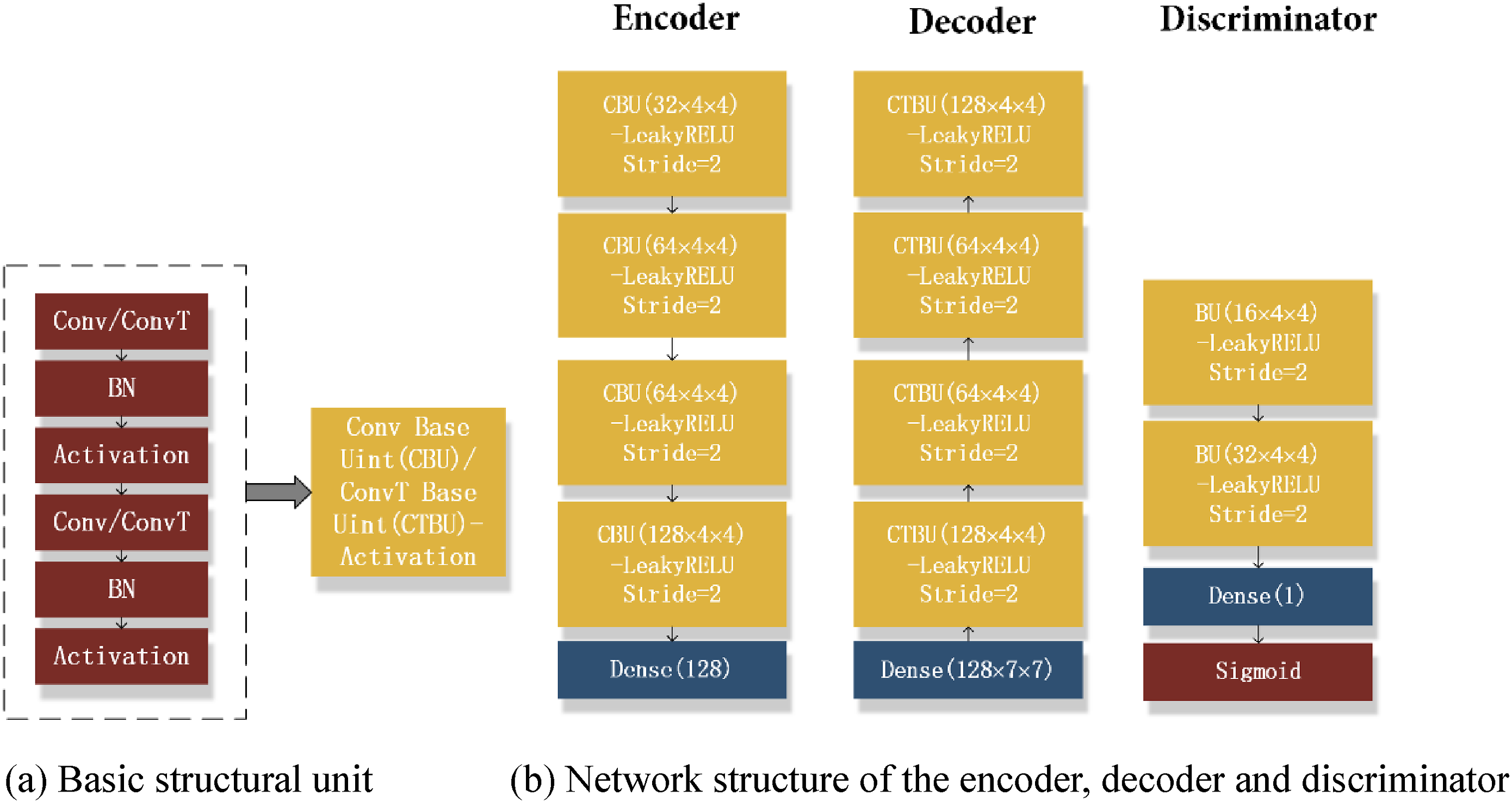

The discriminator network was used to make up the defects of the loss function and improve the sharpness of the generated images. The sigmoid activation function was used to determine whether the images come from real data after the stacking of two basic structural units. The convolution kernel of the discriminator was the same as the encoder in terms of parameter setting principles, and the difference was that the step values of all convolutional layers in the discriminator were set as 2.

The optimization objective consists of three parts. The first part is the data reconstruction loss of the autoencoder module, with the use of the L1 loss function. The second part is the restoration loss of latent space generation features, with the use of the L2 loss function. The third part is the adversarial loss of the discriminator, which is trained by an optimized feature matching method. The three loss functions work together. In summary, the overall loss $L$ of the generator model is:

\begin{array}{l} L = α E_{x \sim p (x)} {‖ x - G (x) ‖}_{1} + {β E}_{x \sim p (x)} {‖ G_{E 1} (x) - G_{E 12} (x) ‖}_{2} + \\ γ E_{x \sim p (x)} {‖ f (x) - E_{x \sim p (x)} f (G (x)) ‖}_{2} \end{array}

(1)

Where,

p (x)

is the real distribution function of the data;

G

is the autoencoder network;

G_{E 12}

represents the generation result from

G_{E 1}

G_{E 2}

; The coefficients

α, β

and

γ

are used respectively to balance the strength of the loss function to ensure the training stability of the model. The test data

x

will be given after training. The anomalous feature

\hat{s}

can be obtained according to the restoration loss of the latent space features

G_{E 1} (\hat{x}) - G_{E 12} (\hat{x})

Extraction of target similarity features

In 1963, Hubel and Wiesel’s research³⁴ showed that the process of cat’s visual information processing presents a hierarchical structure, that is, the front neurons extract simple information and the rear extract complex information. In simulating this process, the deep neural network model is able to extract features layer by layer from simple to complex. The results of visualization research by Matthew et al.³⁵ on the deep convolution model indicate that the features learnt by the layers ranking first mainly include color or edge, while those learnt by the layers ranking behind are texture and more abstract complex ones. Based on the model in the ILSVRC competition, the deep visual features of targets were extracted by the transfer method. This Competition was aimed at testing the object recognition and classification ability of the model by judging the categories of the objects in the images in the 1000 categories in the ImageNet subset. Most of the better models rated in the competitions over the years are deep neural network models.

The Imagenet dataset contains a large number of common target categories, so it can be basically considered the model trained by this dataset and human vision have similar feature extraction capabilities, so that it can be applied to the detection and analysis of military targets. On the other hand, human observers will combine both low-level features and high-level abstract features when detecting targets, so the results extracted from all layers in the network model were sorted from top to bottom and then from left to right to form transfer features. The high-dimensional features after convolution were expressed by calculating the norm (shown in Figure 5).

Figure 5.

Diagram of target similarity feature integration.

Evaluator construction

Supposing the data $x$ was trained by the above two sets of models to form the feature $z_{t r a n}$ , the $z_{t r a n}$ had a large dimension, containing many invalid features. A model was constructed to filter and transform it. First, low variance features were removed to reduce the complexity of the model’s subsequent computation. The threshold was set to 0.1, and the filtered features were denoted as $z_{s}$ . Then, high-rank features were extracted by principal component analysis (PCA). In the feature set $Z_{s} = {z_{s 1}, z_{s 2}, \dots, z_{s n}}_{p \times n}$ formed with all sample sets, $p$ is the feature dimension and $n$ is the number of samples. The $Z_{s}$ was centralized before calculating the covariance matrix of $Σ = \frac{1}{p} Z_{s} {Z_{s}}^{T}$ . The eigenvalues of $Σ$ were decomposed and sorted to obtain the sequence $λ_{1} > λ_{2} > \dots > λ_{p}$ and the eigenvectors corresponding to its eigenvalues. The feature compression degree $ρ_{k}$ was determined according to equation (2).

ρ_{k} = \frac{\sum_{i = 1}^{k} λ_{i}}{\sum_{i = 1}^{p} λ_{i}}

(2)

Where

ρ_{k}

is the degree of feature compression, and

λ

is the eigenvalue. The minimum number of eigenvalues k was determined to be the number of converted features when

ρ_{k} \geq 0.99

. The eigenvectors corresponding

λ_{1}, λ_{2}, \dots, λ_{k}

were combined to be

W = {ν_{1}, ν_{2}, \dots, ν_{k}}^{T}

. The compressed feature

Z_{p c a}

was obtained by equation (3).

Z_{p c a} = W \cdot Z_{s}

(3)

Among them, $Z_{p c a}$ is the compressed feature, $W$ is the feature vector combination, and $Z_{s}$ is the sample feature set. Finally, the method of recursive feature elimination (RFE) was adopted to screen important features. Based on the classification algorithm, this method calculates the importance coefficient of each feature and discards the feature with the smallest coefficient. Non-important features were removed recursively to the set minimum number of features to keep. After the calculation training, the average accuracy rate was calculated through cross-validation, and the model with the highest average rate is finally determined as the final model. The flow chat of the method is shown in Figure 6.

Figure 6.

Flowchart of the RFE algorithm.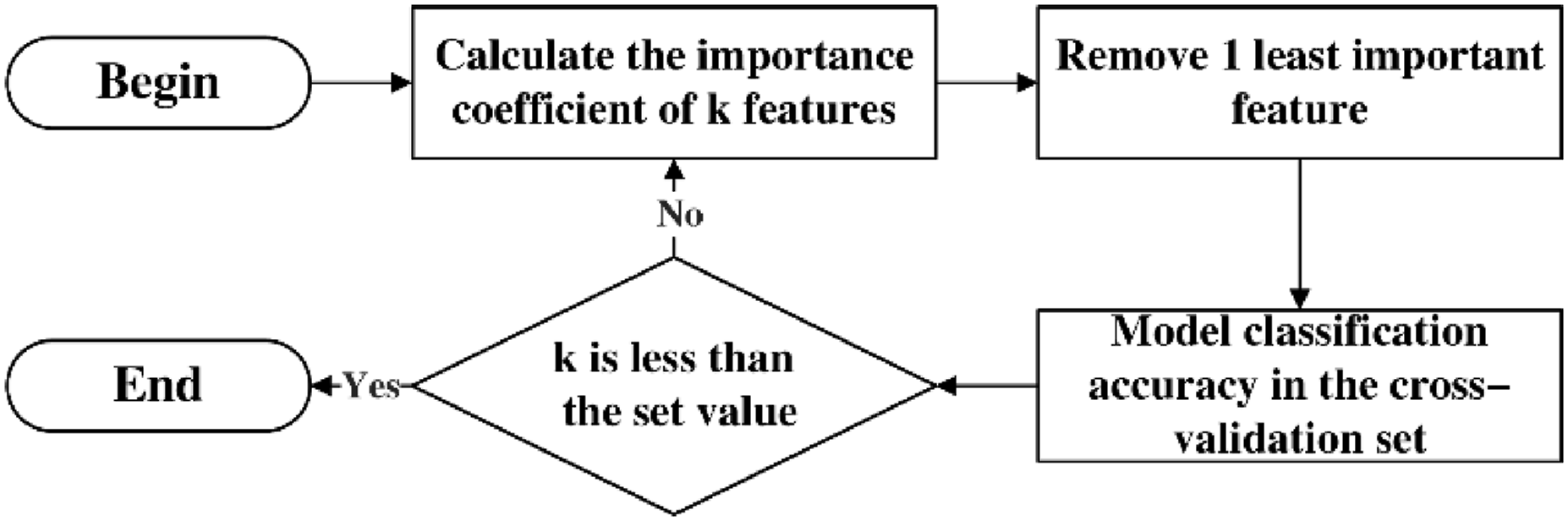

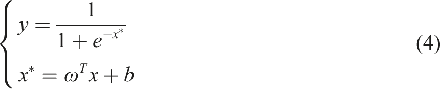
The Logistic Regression³⁶ mode was adopted as a classification mode. The function family adopted in this model is shown in equation (4), in which a nonlinear sigmoid function is added to the result of the linear model.

{\begin{cases} y = \frac{1}{1 + e^{- x^{*}}} \\ x^{*} = ω^{T} x + b \end{cases}

(4)

\min l = \sum - (\hat{y} \log y + (1 - \hat{y}) \log (1 - y))

(5)

Among them,

l

is the cross entropy loss,

y

is the prediction result, with the value of

(0, 1)

;

x

is the input feature;

x^{*}

is the output feature;

ω

and

b

are the parameters to be trained;

\hat{y}

is the true class of the sample, with the value of 0 or 1.

Experiment and result analysis

The target datasets were divided into a training set and a test set at a ratio of 9:1. A 3:1 cross-validation method was applied to the training set for model optimization. The two groups of models were trained separately and then combined for performance test.

Model training and performance optimization

Background differential feature model

Due to the large scale, the model is difficult to complete at once, so the training included two steps. First, the encoder $G$ and the discriminator $D$ were pre-trained separately, and then the learning rate was reduced to 0.1 time for the subsequent joint training with the Adam algorithm. During pre-training, the first-order momentum was set to 0.0001, and the second was set to 0.5. The generation model and the discrimination model were trained alternately after their association. Figure 7 shows the original background data (top column) and the images generated by the encoder $G$ (bottom column). Figure 7(a) shows the images generated in the pre-training. Figure 7(b) shows the images generated after the association with the encoder $D$ . The intuitive results reveal that that the clarity of the images generated by the model was improved to a certain extent after the association with the encoder, which means that the generation ability of the model is further optimized.

Figure 7.

Background images (top row) and model-generated images (below).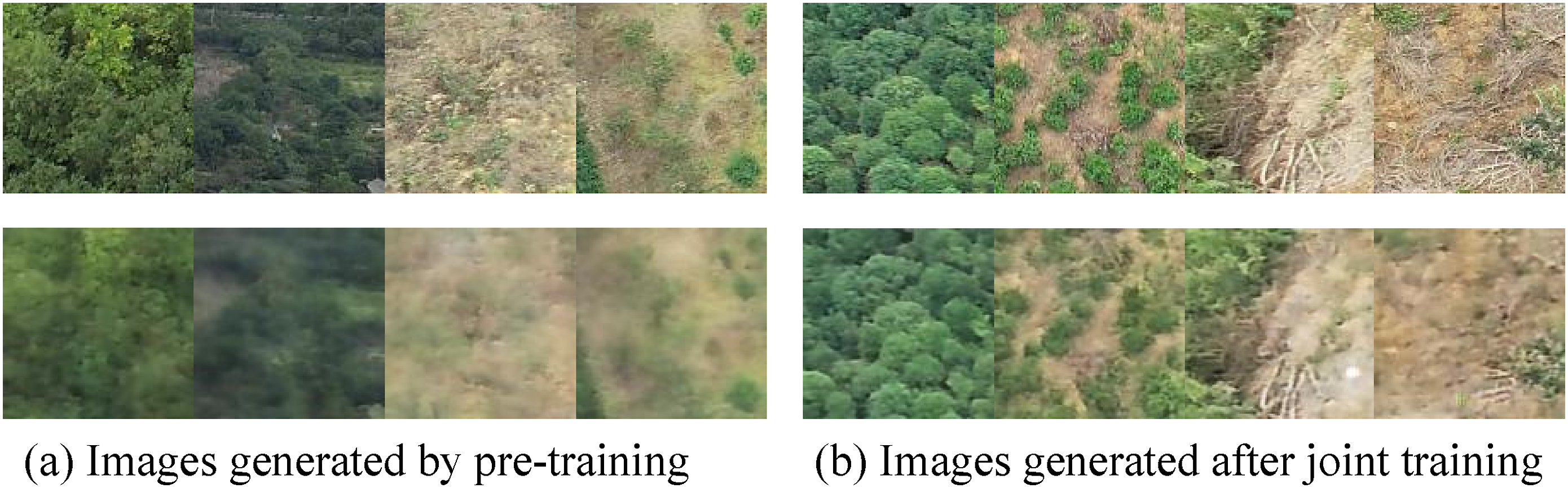

After the training, the target training set was input into the model to obtain and the results shown in Figure 8. Figure 8(a) shows the target images at the level 1 camouflage, and Figure 8(b) shows the target images at levels 2 and 3 camouflages. The upper row shows the original target data; the middle row shows the results reconstructed by the generator; the lower row shows the difference-highlighted grayscale images formed by normalization based on the obtained Euclidean distance color differences in the RGB space between the original and reconstructed images. The intuitive results after reconstruction shows that the reconstruction effect of the levels 2 and 3 camouflage images is obviously poorer than that of the level 1 camouflage images, and the target area cannot be reconstructed well. The target contours can be clearly distinguished in some of the levels 2 and 3 camouflage datasets in the difference-highlighted images, indicating that there are large reconstruction differences in the target areas.

Figure 8.

Target datasets (upper row), reconstruction results (middle row) and difference-highlighted images (lower row).

The Euclidean distance metric between the feature $\hat{z}$ generated by the model and the reconstructed feature $\hat{z}$ ′ was acquired to form the outlier $v_{a b}$ of the sample (see Equation (6)). After the normalization of the obtained outliers $v_{a b}$ of all target datasets, they were divided into two groups to plot the histogram of $v_{a b}$ , and to fit its probability density function. The first group includes the level 1 camouflage sample set, and the second group includes the levels 2 and 3 camouflage sample sets. The kernel density estimation algorithm was adopted for the probability density function, and the Gaussian function was adopted for the kernel function, with the bandwidth set to 0.03. The results demonstrate that the model trained by the background data can discriminate the target data of different camouflage levels to a certain extent. However, it is necessary to construct a classifier on the basis of target datasets since the model can only train background but cannot understand camouflage patterns (Figure 9).

v_{a b} = {‖ \hat{z} - \hat{z}^{'} ‖}_{2}^{2}

(6)

Figure 9.

Statistical histogram and density function of feature outliers in the training set.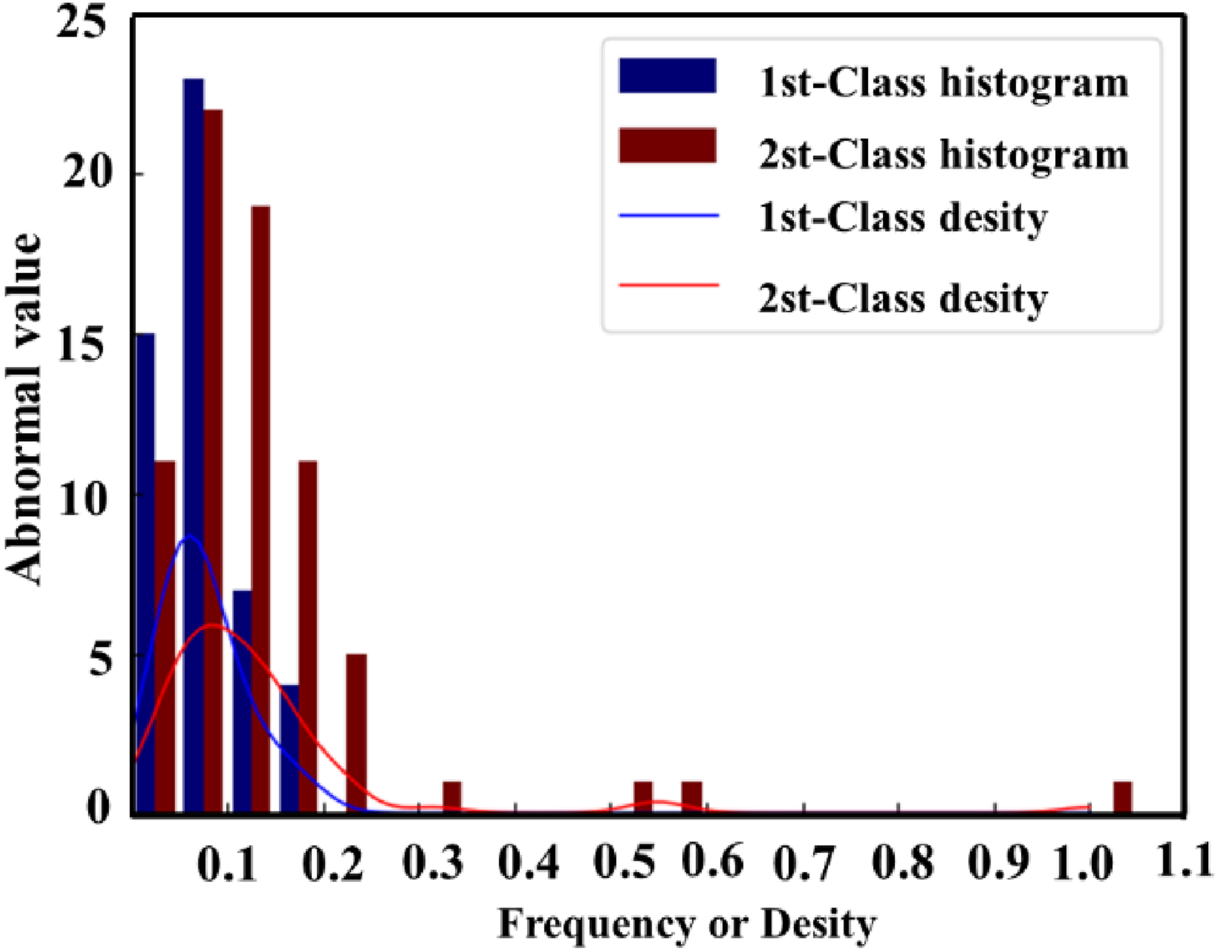

Among them, the outlier of the sample is $v_{a b}$ , $\hat{z}$ is the model generated feature, and $\hat{z}$ ′ is the model reconstructed feature.

The extracted features were first analyzed by PCA, and then the eigenvalues of the covariance matrix were solved and sorted in a descending order, as shown in Figure 10. The eigenvalues before the 80th dimension met the requirements set by equation (2), so the 128-dimensional features were reduced to the 80-dimensional ones through PCA transformation. The model was trained in the cross-validation set to obtain the results shown in Figure 11. The classification accuracy rate (Accuracy), namely the ratio of the number of the camouflage levels predicted accurately to all targets, was used to judge the model. The highest classification accuracy researched 86.8% when 28 features were selected.

Figure 10.

PCA feature values of the training set feature.

Figure 11.

Average accuracy of RFE.

Target difference feature model

The results generated by the three architectures of the VGG16,³⁷ InceptionV3³⁸ and MobileNetV2³⁹ were tested and compared in the experiment on the evaluation model of target feature similarity. Figure 12 shows the variance results of the features at each dimension in the sample training set after the migration of the three models, in which the horizontal coordinate represents the basic feature of each model. Let the feature variance be $v a r$ and the ordinate be $\log (1 + v a r)$ . The reason for this treatment is that the variance values between the various features cannot be limitedly displayed in the figure due to the large differences. It can be seen from the results that the high variance features of the VGG16 model are concentrated in the front; the high variance features of the InceptionV3 model are concentrated in the rear; the feature variance distribution of the MobileNetV2 model is relatively uniform. However, in general, the feature data of the three models are characterized by large interval differences, high dimensions and existence of many invalid features or zero-value features. Therefore, PCA was used for further optimization.

Figure 12.

Feature variance scatter plots of the three models on the training set.

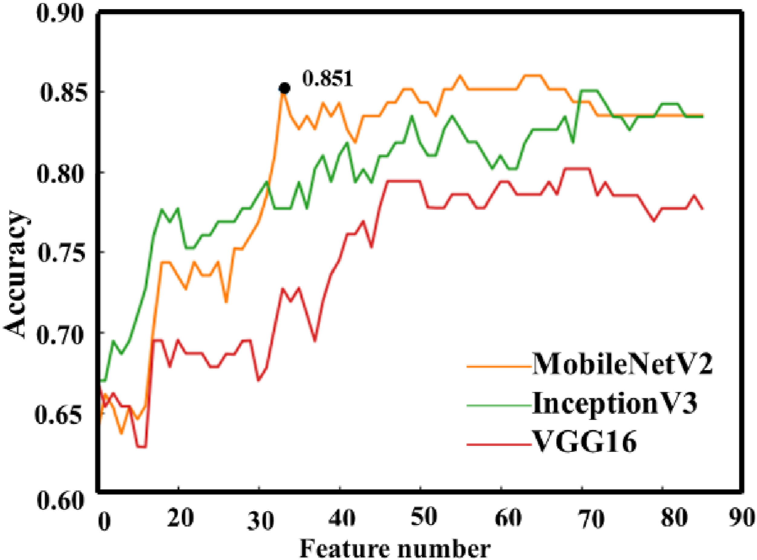
Similarly, the features extracted from the three models were first analyzed by PCA, and the eigenvalues of their covariance matrices were solved and sorted in a descending order, as shown in shown in Figure 13. The eigenvalues before the 85^th dimension met the requirements set by equation (2), so the features are reduced to 85-dimensional ones through PCA transformation. The model was trained in the cross-validation set to obtain the result in the Figure 14. The classification accuracy rate (Accuracy), namely the ratio of the number of the camouflage levels predicted accurately to all targets, was used to judge the model. Overall, the MobileNetV2 in the three models maintains high accuracy for the different numbers of features (see Figure 14). In the average accuracy curve graph, there are two points with high accuracy: the number of features is 33 with an accuracy of 0.851, and the number of features is 57 with an accuracy of 0.859. The accuracy was only improved by 0.8% when the features increase by 73%, and overfitting is prone to happening when there are too many features, so the feature number was set to 33 finally, with the highest cross-validation classification accuracy of 85.1%.

Figure 13.

PCA feature values of the three model output features on the training set.

Figure 14.

RFE average accuracy of the three models.

Comparison of camouflage effect evaluation

The two groups of models were combined to test their final rating performance. Let the output of the background difference model be $f_{b} = G_{b} (x)$ , the output of the target similarity model be $f_{t} = G_{t} (x)$ , the value range of $f_{b}$ and $f_{t}$ be [0, 1]. The result of $f_{b}$ close to one indicated that x was level 1 camouflage, while $f_{t}$ close to one indicated that x was level 3 camouflage. When $P_{p r o b}$ was set as the probability value of the final prediction, $P_{p r o b}$ was a 3-dimensional vector. Each element was associated with the probability value of the corresponding level. Their results can be calculated according to equation (7). 0.5 was taken as a threshold value to discuss in three case: if $f_{b} > 0.5$ , the model $G_{b}$ played a major role, so let the level 1 probability be $f_{b}$ , and distribute the probability values generated by $G_{t}$ to the levels 1 and 2 equally and ensure that all probabilities summed to 1; when $f_{t} > 0.5$ , the model $G_{t}$ played a major role, so let the level 1 probability be $f_{t}$ , and distribute the probability values generated by $G_{b}$ to the levels 1 and 2 equally and ensure that all probabilities sum to 1. When both $f_{b}$ and $f_{t}$ were less than 0.5, so let the level 2 probability be the average value $1 - (f_{t} + f_{b}) / 2$ of the two models, and the levels 1 and 3 probabilities be $f_{b} / 2$ and $f_{t} / 2$ respectively. Thereby, the probability matrix $P_{p r o b}$ of all samples can be completely generated.

P_{p r o b} = {\begin{cases} [f_{b}, (1 - f_{b}) \cdot (1 - f_{t}), (1 - f_{b}) \cdot f_{t}], i f f_{b} > 0.5 \\ [\frac{f_{b}}{2}, \frac{2 - f_{t} - f_{b}}{2}, \frac{f_{t}}{2}], i f f_{b} < 0.5 a n d f_{t} < 0.5 \\ [(1 - f_{t}) \cdot f_{b}, (1 - f_{b}) \cdot (1 - f_{t}), f_{t}], o t h e r s \end{cases}

(7)

The probability matrix of the sample is $P_{p r o b}$ , $f_{b}$ is the background difference model, and $f_{t}$ is the target similarity model.

The receiver operating characteristic (ROC) curve was used to describe the rating performance of the model. The horizontal coordinates of the curve represent the sensitivity and the vertical ordinates represent the specificity. The closer the curve is to the upper left corner, the better the classifier. The predicted probability of each class target data and their true classes were combined to form a curve graph. Moreover, the overall “micro average” (micro) ROC curve can be obtained by averaging the ROC curves of all classes. After the class labels were converted into a one-hot label matrix $L$ , a ROC curve was formed by unfolding $L$ and the probability matrix $P_{p r o b}$ in rows simultaneously, called the “macro average” (macro) ROC curve. The results of the five curve graphs are shown in Figure 15. According to the results, the model had the best accuracy for classifying level 1 camouflages, and worst best accuracy for classifying level 2 camouflages. The curves generated by the two averaging methods were closer to the upper left, indicating that the classifier performed well.

Figure 15.

ROC curves of the three levels and the two averaged methods.

The accuracy of the classifier was further checked by the confusion matrix (shown in Figure 16), in which the vertical ordinate represented the true class and the horizontal ordinate represented the predicted class. The results indicated that the accuracy of the level 1 classification was the highest, and part of the real level 2 targets were classified into the level 3 ones by mistake. Objectively, the voting rate for part of the level 2 camouflage targets is low in performing camouflage rating. Thus, it can be verified that the classification result of the model is somewhat consistent with that of human observers, which is because of the small size of the target datasets.

Figure 16.

Confusion matrix generated by rating results.

Four types of feature extraction methods such as statistical features, color features, shape features and texture features were selected for comparison with the methods for manually extracting features to build models. For feature statistics, the image entropy $e$ (see Equation (8)) was adopted to describe the richness of image details. In the equation, $p (z)$ is the statistical histogram, and $L$ is the maximum gray scale. The Euclidean distance between two colors in the RGB color space was calculated for color features; Canny operators⁴⁰ were used to extract edge features for shape features; a LBP⁴¹ rotation invariant feature was adopted for texture features; the difference between the target and background could be directly calculated for statistical features. Two-dimensional correlation coefficients were used to calculate the feature similarity $r$ (Equation (9)) for the extracted images of color, shape and texture features (Equation (9)). The 8-connected domain method²⁵ was used to divide the target and the backgrounds, that is, surrounding images of the same size as the target is selected as the backgrounds to calculate the average of the feature similarity between the target and the eight backgrounds, so that four average feature results were obtained.

e = - \sum_{z = 0}^{L - 1} p (z) \log_{2} (p (z))

(8)

r_{x, y} = \frac{\sum_{i} \sum_{i} (x_{i j} - \bar{x}) (y_{i j} - \bar{y})}{{(\sum_{i} \sum_{i} {(x_{i j} - \bar{x})}^{2} \cdot \sum_{i} \sum_{i} {(y_{i j} - \bar{y})}^{2})}^{1 / 2}}

(9)

The image entropy is $e$ , the feature similarity is $r_{x, y}$ , $p (z)$ is the statistical histogram, and $L$ is the maximum grayscale. $x_{i j}$ is the feature map of the target, $\bar{x}$ is the average feature map of the target, $y_{i j}$ is the feature map of the background, and $\bar{y}$ is the average feature map of the background.

The BP network model and linear model were used for fitting respectively. Finally, the Area under the Curve of ROC (AUC) and accuracy indicators were used to compare the performance of the models, and the results are shown in Table 1. The final AUC of the model proposed in this paper was 0.939 for Micro and 0.945 for Macro, and the accuracy of camouflage classification was 84.3%, indicating that the model performed better than the two artificial feature models.

Table 1.

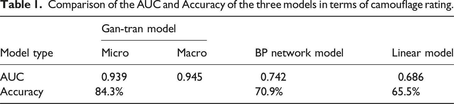
Comparison of the AUC and Accuracy of the three models in terms of camouflage rating.

Model type	Gan-tran model		BP network model	Linear model
Model type	Micro	Macro	BP network model	Linear model
AUC	0.939	0.945	0.742	0.686
Accuracy	84.3%		70.9%	65.5%

The performance of the Gan-Tran method and SSIM, UIQI,⁴² MSE and PSNR similarity evaluation indexes was further investigated. Based on equation (10), the three levels predicted by the target datasets were respectively mapped to [0, 1/3], [1/3, 2/3] and [2/3, 1] to form a continuous numerical result $S_{G - T}$ . In equation (10), $i$ was assigned with values of 1, two and three respectively, corresponding to the three levels of camouflage effect. Furthermore, the similarity between the central target area and the background of the surrounding eight connected domains was calculated and averaged to obtain the final results of the other four indicators. The similarity results of all sample sets were divided into three categories and different levels to form boxplots, as shown in Figure 17.

S_{G - T} = \frac{1}{3} (\arg \max_{i} P_{p r o b} (i) - 1) + \frac{1}{3} \max_{i} P_{p r o b} (i)

(10)

Figure 17.

Similarity boxplots formed by five similarity evaluation methods in the sample sets.

Among them, $S_{G - T}$ is the numerical result, and $P_{p r o b} (i)$ is the probability matrix.

Figure 17 illustrates that that the method proposed in this paper performs the best to distinguish different camouflage levels of targets according to the upper and lower limits, followed by the MSE and PSNR indicators, which can basically reflect the camouflage levels according to the median trends, but with poor distinguishing ability, they cannot distinguish different camouflage levels by taking the upper and lower limits or quartiles as thresholds. The third is the SSIM indicator, which can only distinguish the level 1 camouflage well, since it is only available for the structural similarity between the target and background, but unable to distinguish whether a central area contains target features. The UIQI indicator cannot distinguish camouflage levels. As a result, the method proposed in this paper has better performance than the four evaluation indicators.

Conclusion

Based on the perception experiment method, a manual annotation method for camouflage rating was proposed, thereby constructing target datasets. The target datasets and collected background data were used to construct a deep neural network to extract camouflage features and establish a camouflage effect evaluation architecture model Gan-Tran, which is composed of two sub-models. The GANomaly model that obtains abnormal features by training on the background datasets is used to detect whether the data to be detected is similar to the background image data, so as to define the level 1 camouflage. The MobileNetV2 model features are transferred on the target datasets to check whether the data to be detected is similar to the target data features, so as to define the level 3 camouflage. PCA dimensionality reduction and RFE screening are used to determine the final features, and the logistic regression model was used to obtain final rating results. In the experiment, the accuracy of the GANomaly model was tested separately after the model optimization. The GANomaly model had an accuracy of 86.8% after selecting 28-dimensional features, and the migration model had an accuracy of 85.1% after selecting 33-dimensional features. The final classification accuracy of the two models associated was 84.3% on the test sets, and the Micro and Macro AUC values reached 0.939 and 0.945, respectively, indicating that they better classification performance than the BP network model and the linear model constructed by the artificial feature model. In addition, according to the calculated results of the four indicators of SSIM, UIQI, MSE and PSNR, Gan-Tran can classify camouflage levels better. The method can be applied to the evaluation and rating of optical camouflage effects of national defense projects and combat targets. The next study is to optimize the dataset to further improve the reliability and stability of the model. This method can provide optimization solutions for color and pattern printing of military combat textiles such as camouflage work clothes and camouflage nets.

Footnotes

Declaration of conflicting interests

The author(s) declared no potential conflicts of interest with respect to the research, authorship, and/or publication of this article.

Funding

The author(s) disclosed receipt of the following financial support for the research, authorship, and/or publication of this article: This work was supported by the key Project on Battlefield Visibility Control and Unidirectional Transmission technology (KYGYJKQTZQ23007).

ORCID iD

Bentian Hao

References

Aurdal

Lokken

Klausen

, et al. Adversarial camouflage for naval vessels. Artificial intelligence and machine learning in defense applications. 2019; 11169: 163–174. SPIE. DOI: 10.1117/12.2532756.

Cheng

X-p.

Shu

B-w.

Chang

Y-j.

, et al. Evaluation of infrared camouflage effectiveness via a multi-fractal method. Defence Technology 2021; 17(3): 748–754. DOI: 10.1016/j.dt.2020.05.006.

Cuthill

. Camouflage. J Zool 2019; 308(2): 75–92. DOI: 10.1111/jzo.12682.

Hogan

Cuthill

Scott-Samuel

. Dazzle camouflage, target tracking, and the confusion effect. Behav Ecol 2016; 27(5): 1547–1551. DOI: 10.1093/beheco/arw081.

Font

. Mimicry, camouflage and perceptual exploitation: the evolution of deception in nature. Biosemiotics 2019; 12(1): 7–24. DOI: 10.1007/s12304-018-9339-6.

Neider

Sarno

Lewis

, et al. Training detection of camouflaged targets in natural scenes: backgrounds and targets both matter. Acta Psychol 2021; 219: 103394. DOI: 10.1016/j.actpsy.2021.103394.

Jun

Haoyang

Yunhui

, et al. An evaluation method of optical camouflage effect based on contour deformation degree. Acta Photonica Sin 2021; 50(6): 196–204.

Feng

Guoying

Richang

, et al. Camouflage texture evaluation using a saliency map. Multimed Syst 2015; 21(2): 169–175. DOI: 10.1007/s00530-014-0368-y.

Wei

Wang

. A novel method for automatic camouflage pattern synthesize. IEEE Access 2021; 9: 67559–67568. DOI: 10.1109/ACCESS.2021.3077258.

10.

Mondal

. Camouflage design, assessment and breaking techniques: a survey. Multimed Syst 2022; 28(1): 141–160. DOI: 10.1007/s00530-021-00813-6.

11.

Volonakis

Matthews

Liggins

, et al. Camouflage assessment: machine and human. Comput Ind 2018; 99: 173–182.

12.

Chao-chao

Jiang-hua

Guang-zhen

. Texture feature extraction method of camouflage effect evaluation model. Command Control & Simulation 2017; 39(3): 4.

13.

Bai

Liao

. Assessment of camouflage effectiveness based on perceived color difference and gradient magnitude. Sensors 2020; 20(17): 20174672. DOI: 10.3390/s20174672.

14.

Gan

Liu

, et al. An evaluation method of dynamic camouflage effect based on multifeature constraints. IEEE Access 2020; 8: 193845–193855. DOI: 10.1109/ACCESS.2020.3025801.

15.

Prasetyo

YT.

Evaluating existing China military camouflage designs using camouflage similarity index (CSI). In: 5th International Conference on Industrial and Business Engineering (ICIBE), 27–29 September 2019, Hong Kong,, pp. 321–325.

16.

Songlin

Yuhua

Jijun

, et al. Research on optical image similarity evaluation based on multi-feature statistics. Protective Engineering 2020; 42(195): 62–67.

17.

Jiaju

Yongqiang

Yudan

, et al. Evaluatiuon of infrared dynamic camouflage effect based on feature synthesis. Semicond Optoelectron 2019; 3: 5.

18.

Jia-Kun

Yan-Bin

Hai-Rui

, et al. Set pair evaluation model for optical camouflage effect of air defense missile equipment. Laser & Infrared 2019; 49(5): 6.

19.

Jin

Li-Fan

Hai-Lu

. Evaluation model of optical camouflage effect based on BP neural network. Shipboard Electronic Countermeas Ure 2009; 32(6): 3.

20.

Florencio

Zhao

, et al. Foreground detection in camouflaged scenes. In: 2017 24th IEEE international conference on image processing (ICIP), 17–20 September 2017, Beijing, 2017, pp. 4247–4251.

21.

Stuart

Yip

Hogendoorn

. The role of hue in visual search for texture differences: implications for camouflage design. Vis Res 2020; 176: 16–26. DOI: 10.1016/j.visres.2020.07.008.

22.

Yan

T-N

Nguyen

K-D

, et al. MirrorNet: bio-inspired camouflaged object segmentation. IEEE Access 2021; 9: 43290–43300. DOI: 10.1109/ACCESS.2021.3064443.

23.

Richter

Goncalves

Gomes

NAS

. Effect of combat textile cloth on human radar cross section for microwave camouflage applications. Journal of Defense Modeling Simulation 2023; 20: 415–422. DOI: 10.1177/15485129221077432.

24.

Jia

, et al. Design and evaluation of digital camouflage pattern by spot combination. Multimed Tool Appl 2020; 79(29-30): 22047–22064. DOI: 10.1007/s11042-020-09002-5.

25.

Yang

Jia

, et al. MF-CFI: a fused evaluation index for camouflage patterns based on human visual perception. Defence Technology 2021; 17(5): 1602–1608.

26.

Yan

. Restoration of images corrupted by impulse noise and mixed Gaussian impulse noise using blind inpainting. SIAM J Imag Sci 2013; 6(3): 1227–1245.

27.

Yang

W-D

Liu

, et al. Simulation evaluation method for fusion characteristics of the optical camouflage pattern. Fibres Text East Eur 2021; 29(3): 103–110. DOI: 10.5604/01.3001.0014.7795.

28.

Xiaofeng

Yebin

, et al. An infrared stealth camouflage evaluation method basedon improved gradient similarity. Electron Opt Control 2022; 29(02): 7–11.

29.

Jiao

, et al. Research status and development trend of image camouflage effect evaluation. Multimed Tool Appl 2022; 81: 29939–29953. DOI: 10.1007/s11042-022-12287-3.

30.

Hall

Matthews

Volonakis

, et al. A platform for initial testing of multiple camouflage patterns. Defence Technology 2021; 17(6): 1833–1839. DOI: 10.1016/j.dt.2020.11.0042214-9147.

31.

Toet

Hogervorst

. Review of camouflage assessment techniques. Target and background signatures VI. 2020; 11536: 1153604. DOI: 10.1117/12.2566183.

32.

Akcay

Atapour-Abarghouei

Breckon

. GANomaly: semi-supervised anomaly detection via adversarial training. Computer Vision - ACCV 2018; 2019: 622–637.

33.

Szegedy

Ioffe

Vanhoucke

, et al. Inception-v4, inception-ResNet and the impact of residual connections on learning. In: AAAI conference on artificial intelligence, 4–9 February 2017, San Francisco, 2016.

34.

Hubel

Wiesel

. Receptive fields, binocular interaction and functional architecture in the cat's visual cortex. J Physiol 1962; 160(1): 106–154.

35.

Zeiler

Fergus

. Visualizing and understanding convolutional networks. Computer Vision - ECCV 2014; 2014: 818–833.

36.

Hosmer

, et al. A comparison of goodness-of-fit tests for the logistic regression model. Stat Med 2015; 16(9): 965–980.

37.

Srivastava

Kumar

Chaudhry

, et al. Detection of ovarian cyst in ultrasound images using fine-tuned VGG-16 deep learning network. SN Computer Science 2020; 1(2): 81. DOI: 10.1007/s42979-020-0109-6.

38.

Joshi

Tripathi

Bose

, et al. Robust sports image classification using InceptionV3 and neural networks. Procedia Comput Sci 2020; 167: 2374–2381.

39.

Sandler

Howard

Zhu

, et al. MobileNetV2: inverted residuals and linear bottlenecks. In: 2018 IEEE/CVF conference on computer vision and pattern recognition (CVPR), June 2018, Salt Lake, 2018, pp. 4510–4520.

40.

Yan

, et al. Self-adaptive Canny operator edge detection technique. Journal of Harbin Engineering University 2008; 29(9): 1002–1007.

41.

Lis

Black

Korn

, et al. Association between sitting and occupational LBP. Eur Spine J 2007; 16(2): 283–298.

42.

Lin