A field development strategy for the joint optimization of flow allocations,well placements and well trajectories

Abstract

One of the major goals that field planning engineers and decision makers have to achieve in terms of reservoir management and hydrocarbon recovery optimization is the maximization of return on financial investments. This task yet very challenging due to high number of decision variables and some uncertainties, pushes the engineers and technical advisors to seek for robust optimization methods in order to optimally place wells in the most profitable locations with a focus on increasing the net-present value over a project life-cycle. The quest to deliver a good quality advice is also dependent on how some uncertainties – geologic, economic and flow patterns – have been handled and formulated all along the optimization process. With the enhancement of computer power and the advent of remarkable optimization techniques, the oil and gas industry has at hand a wide range of tools to get an overview on value maximization from petroleum assets. Amongst these tools, genetic algorithms which belong to stochastic optimization methods have become well known in the industry as one the best alternatives to apply when trying to solve well placement and production allocation problems, though computationally demanding. The aim of this work is to present a novel approach in the area of hydrocarbon production optimization where control settings and well placement are to be determined based on a single objective function, in addition to the optimization of wells’ trajectories. Starting from a reservoir dynamic model of a synthetic offshore oil field assisted by water injection, the work consisted in building a data-driven model that was generated using artificial neural networks. Then, we used Matlab’s genetic algorithm toolbox to perform all the needed optimizations; from which, we were able to establish a drilling schedule for the set of wells to be realized, and we made it possible to simultaneously get the well location and configuration (vertical or horizontal), well type (producer or injector), well length, well orientation – in the horizontal plane –, as well as well controls (flow rates) and near wellbore pressure with respect to a set of linear and nonlinear-constraints. These constraints were formulated so as to reproduce real field development considerations, and with the aid of a genetic algorithm procedure written upon Matlab, we were able to satisfy those constraints such as, maximum production and injection rates, optimal wellbore pressures, maximum allowable liquid processing capacity, optimal well locations, wells’ drilling and completion maximum duration, in addition to other considerations. We have investigated some scenarios with the intention of proving the benefits of development strategy that we have chosen to study. It was found the chosen scenario could improve NPV by 3 folds in comparison to a base case scenario. The positioning of the wells was successful as all producers were placed in zones having initial water saturation less than 0.4., and all injectors were placed high water saturation zones. Moreover, we established a procedure regarding well trajectory design and optimization by taking into account, minimum dogleg severity and maximum duration for a well to be drilled and completed with respect to a time threshold. The findings as well as the workflow that will be presented hereafter could be considered as a guideline for subsequent tasks pertaining to the process of decision making, especially when it has to do with the development of green oil and gas fields and will certainly help in the placement of wells in less risky and cost-effective locations.

Introduction

Following the multiple achievements carried out in the area of field development planning (FDP), there is still much to do in terms of the optimization of well placement, drilling schedule and flowrate allocation (production/injection), in order to deliver to managers and decision-makers a detailed reservoir management strategy aiming to the maximization of oil production and return on investment throughout the entire lifecycle of an oil or gas field. This process is usually very challenging depending on the level of complexity of hydrocarbon reservoirs (heterogeneous, fractured, multi-layered) and necessitates some experience, good judgment and lessons learnt for the optimal placement of new wells, and is traditionally performed through time-consuming simulation runs for a number of scenarios under a large set of constraints and uncertainties.

A lot of researchers and petroleum practitioners have published numerous works on the joint optimization problem of well placement and flow allocation using evolutionary algorithms, mainly genetic algorithms (GA), and other promising method. Most of the papers that are going to be cited used a dynamic reservoir simulation while only few dealt with the use of proxy models or surrogate models – such as machine learning (ML) models – to estimate oil production from hydrocarbon reservoirs.

Concerning field development optimization using reservoir simulation, Awotunde (2014b) used a differential evolution algorithm for the joint optimization problem. A well control zonation was combined with four reduction models to determine well types and configurations according to different problem size dimensions. This work was further developed by Awotunde (2014c, 2014d) using the CMA-ES optimization algorithm (Covariance-Matrix Adaptation Evolutionary Strategy) with the integration of minimum well spacing constraint, well schedule and project life in the net-present value formulae. Alghareeb et al. (2014) applied an original evolutionary algorithm called “Modified Cuckoo Search (MCS)” on two cases involving synthetic reservoir models. The results indicated that applying the MCS algorithm performs better than GA in finding optimal solutions and that the integration of a filtering technique to that algorithm enables to find feasible solutions fastly. The MCS algorithm was also compared to PSO, CMA-ES and GPS (Global Pattern Search) and the same findings were reported by Wang et al. (2016). Awotunde et al. (2018) proposed to incorporate regional pressure balance constraint in order to have a homogeneous pressure-balanced region inside a reservoir. A differential evolution algorithm was used to evaluate several field development cases. Their findings indicated that having a pressure-balanced region will yield a lower net-present value (NPV) than a non-balanced region. The same conclusion was reported by Awotunde (2014a). Hutahaean (2014) and Hutahaean et al. (2014) investigated the effect of sulphate scale deposition on well placement optimization in an oil reservoir assisted by waterflooding using particle swarm optimization (PSO). They showed that this approach allows to easily spot location with low-risk scale deposition and high oil recovery. Jesmani et al. (2014) used the PSO algorithm on two different reservoirs in order to investigate the effect of inter-well distance, well length, well orientation and reservoir bounds. These constraints were handled using a decoder constraint-handling method. It was found that adding a decoder will lead to lower computational costs in comparison to filtering methods. Lu and Reynolds (2019) applied GA for the joint optimization problem of well positioning, well type, drilling order and control settings in two different reservoirs. It was found that the GA produces different optimal solutions at each run with a small relative change in the NPV. Morales et al. (2011) proposed a modified GA for the optimization of well placement under geologic uncertainty. Their approach consisted in introducing a risk-level criterion for well positioning in order to spot zones with low risk level, i.e., zones with high economic value. Also, they highlighted that the modified GA proved to be a robust tool when dealing with geologic uncertainties. Khoshneshin and Sadeghnejad (2018) investigated two optimizers, PSO and Artificial Bee Colony (ABC), to find the best drilling location of a new well. These two optimizers were applied on two successive development scenarios (exploration phase and infill drilling phase). It was found that ABC is more likely to yield a higher NPV than PSO. Li and Jafarpour (2012) solved the joint optimization problem by finding simultaneously feasible solutions for the control setting and well positioning joint problem. A well distance constraint was introduced to the NPV function as a penalty function and the objective function was reformulated to a series of non-linear functions.

The joint optimization problem was also investigated by means of machine learning-based proxy models. Leeuwenburgh et al. (2010) investigated several “Ensemble Methods” for well placement and production optimization of two synthetic fields – a homogeneous sealed reservoir and a heterogeneous reservoir - assisted by water alternating gas (WAG). Their approach took into consideration geologic uncertainty and the results indicated that simultaneous optimization performs better than a sequential approach yet computational costs were nearly the same. Jang et al. (2017) used sequential artificial neural network (ANN) to optimize the placement of a horizontal well in a coalbed methane reservoir. Their findings indicated that this approach required fewer runs to achieve a global solution in comparison to the PSO algorithm. Memon et al. (2014) investigated a surrogate reservoir model based on radial basis neural network (RBNN) in order to predict dynamic bottom-hole pressure in a multilayer reservoir under a set of production and injection constraints. The results reported that RBNN are powerful in replicating the same results as obtained by a dynamic reservoir simulation. Nwachukwu et al. (2018a, 2018b) proposed a reservoir proxy model based on a gradient boosting method for solving well positioning and control settings challenge using an optimization algorithm called “Mesh Adaptive Direct Search (MADS)”. It was proved that the simultaneous optimization of flow allocation and well placement is very efficient and no computational costs were noticed in comparison to the sequential approach. A good correlation was also found between their proxy model and reservoir simulation. Considering analytical solution-based proxy model, Alrashdi and Stephen (2020) used a proxy model, based on some analytical solutions to a 2D flow problem, for the optimization of well placement and rate controls. Formulas derived from the buckly-Leverett (BL) equation and declined curve analysis (DCA) were compared the ouput of a reservoir simulator. The focus of this paper was to show how an analytical-based approach is likely to mimic results given by conventional simulator. It was also pointed out that an engineering-based well positioning approach could improve the NPV in comparison to a manual approach.

The aim of this study is to seek for optimal flow settings and well locations in order to set a strategy for the development of a virtual offshore oil field. The joint optimization problem of well placement and flow allocation, in contrast to Forouzanfar and Reynolds (2014), will be solved all together in one stage. Hence, differently to what was found in the literature and to what was carried out by Forouzanfar and Reynolds (2013), the aim of our simplified approach was achieved by generating a unique function that combines and allows getting simultaneously and at each time-step:

Drilling schedule.

Well location.

Well type and geometry.

Well length and orientation in space.

Flow allocation and the corresponding wellbore pressure to operate each well at that flowrate.

The optimization process was carried out based on a mixed integer formulation including numerical and categorical variables. The approach consists in building a RBNN function using Matlab’s ANN toolbox in order to get a correlation - from a statistical standpoint - between the aforementioned variables and the target of interest, in our case, near-wellbore pressure. In order to achieve this, the whole optimization process will be carried out using Matlab’s GA toolbox with respect to a set of linear and non-linear constraints, such as:

Geometric limits.

Minimum well distance.

Initial water saturation.

Maximum duration for drilling and completion activities.

The proposed strategy will be compared to some scenarios in order to see which option is going to theoretically yield maximum revenues. In addition to this, a well trajectory optimization methodology will be presented, where we will show how to get optimal well path and well length under a critical dogleg severity, as well as the duration required for drilling and completing a well. This task will be performed sequentially along with the joint optimization of flow allocation and well placement.

Methodology

Presentation

The proposed ANN approach was made possible by collecting some soft data obtained through the simulation of a synthetic water flooded oil reservoir located offshore. The neural network illustrated by Figure 1, which is a representation of a well model, was trained using 3024 observations then validated over 1296 observations. The set of predictors that were chosen allows determine a complete drilling schedule with time “t” for a well to be drilled, in addition well location (x, y, z), well type (producer/injector), geometry (vertical/horizontal), length of well segment that is in contact with the reservoir, well orientation in XY plane (only for horizontal wells), the flow allocated to it and finally, the near-wellbore pressure. The ANN model sketched in Figure 1, which is a simplistic representation of a neural net, was modelled using radial based neural networks (RBNN) on Matlab to predict bottom-hole pressure on each well at each time based on the aforementioned inputs.

Figure 1.

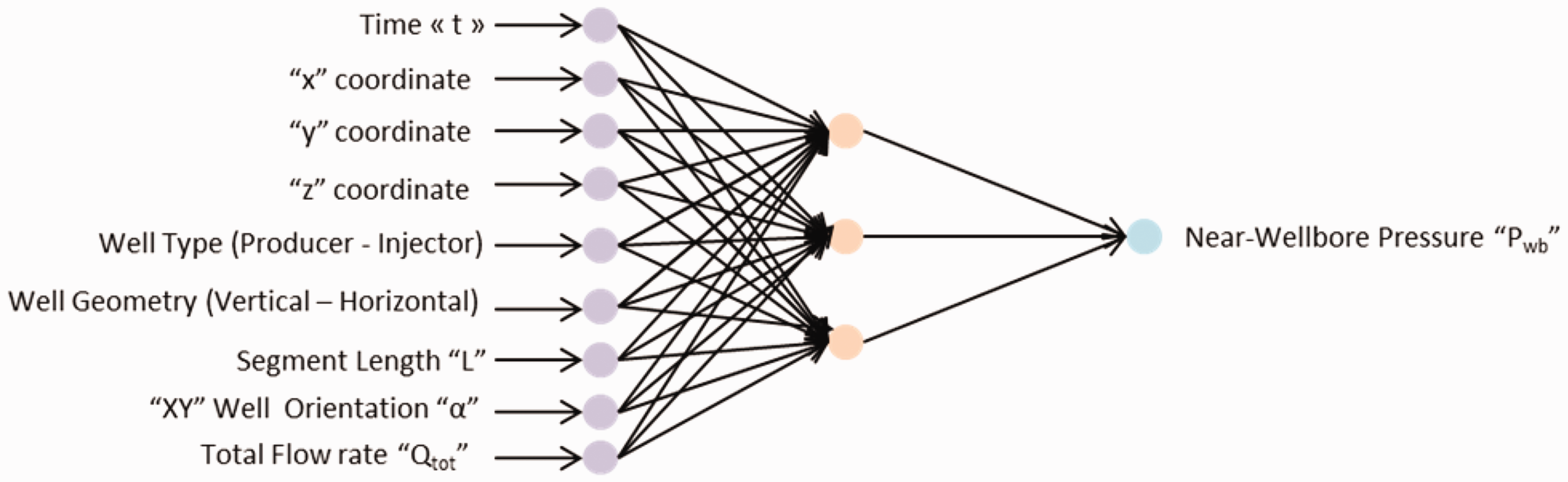
ANN representation of a well model.

Similar to conventional feed forward networks, RBNN consists of an input layer, a hidden layer and an output layer. The hidden layer uses a non-linear radial basis function as an activation function. As sketched in Figure 1, we started by three hidden layers, but the RBNN is designed so that when fitting this neural net to the data, the total number of hidden layers will be increased till achieving a predefined mean square error threshold. The final number of hidden neurons will be shown later in this paper.

Genetic algorithm – A brief description

Genetic algorithms are well developed and robust optimization methods used widely in several areas of research to solve problems. GA are based on natural selection where an optimal solution, - an optimal population of offspring - is obtained or derived from an initial population (i.e., parents) through a stochastic optimisation process of natural selection.

GA evolves the initial population of decision variables via a genetic transformation process, by means of selection, mutation and crossover; and the final offspring population is achieved when we get the highest fitness which is in our case, the net-present value. Hence, the final offspring will be considered as the solution to the optimization problem.

Figure 2 shows a general flowchart of GA. After evolving several generations, the population having individuals with highest fitness value will be considered as the optimal values of the decision variable. These optimal values (final offspring population) will be met when the average relative change in the best fitness function value is less than a function tolerance or the maximum number of generation is achieved.

Figure 2.

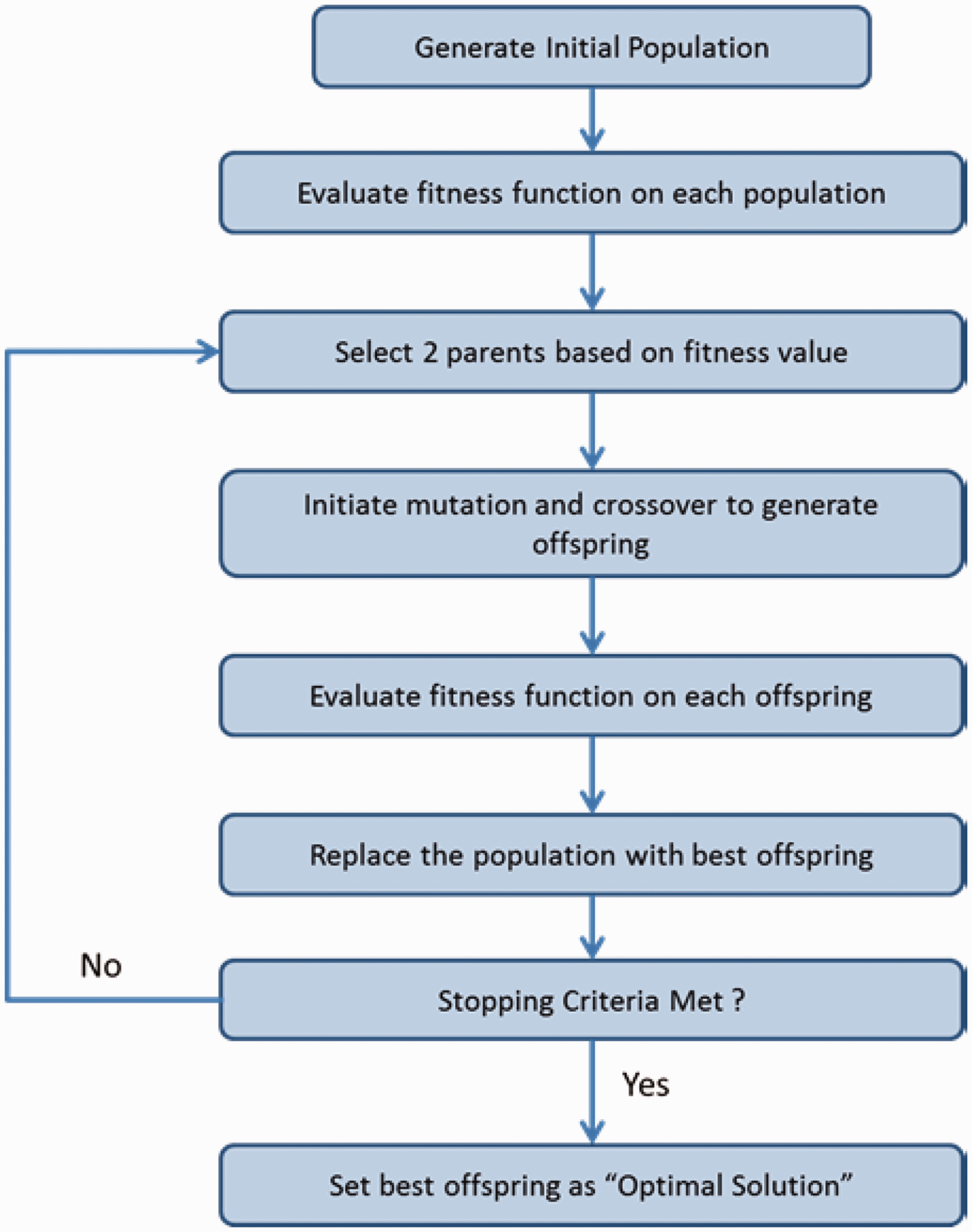
Genetic Algorithms flowchart.

Algorithmic procedure

The main purpose of this study is to seek for optimal locations to place producers and injectors in an oil reservoir with the aim of having at the end of the life-cycle of a field, as significant NPV as possible. Basically, a well consists of 2 segments (Figure 3): a first segment – the dashed line – that is in contact with the reservoir and where fluids will flow through, and a second segment – the continuous line – that goes from the point where the reservoir has been targeted, up to surface.

Figure 3.

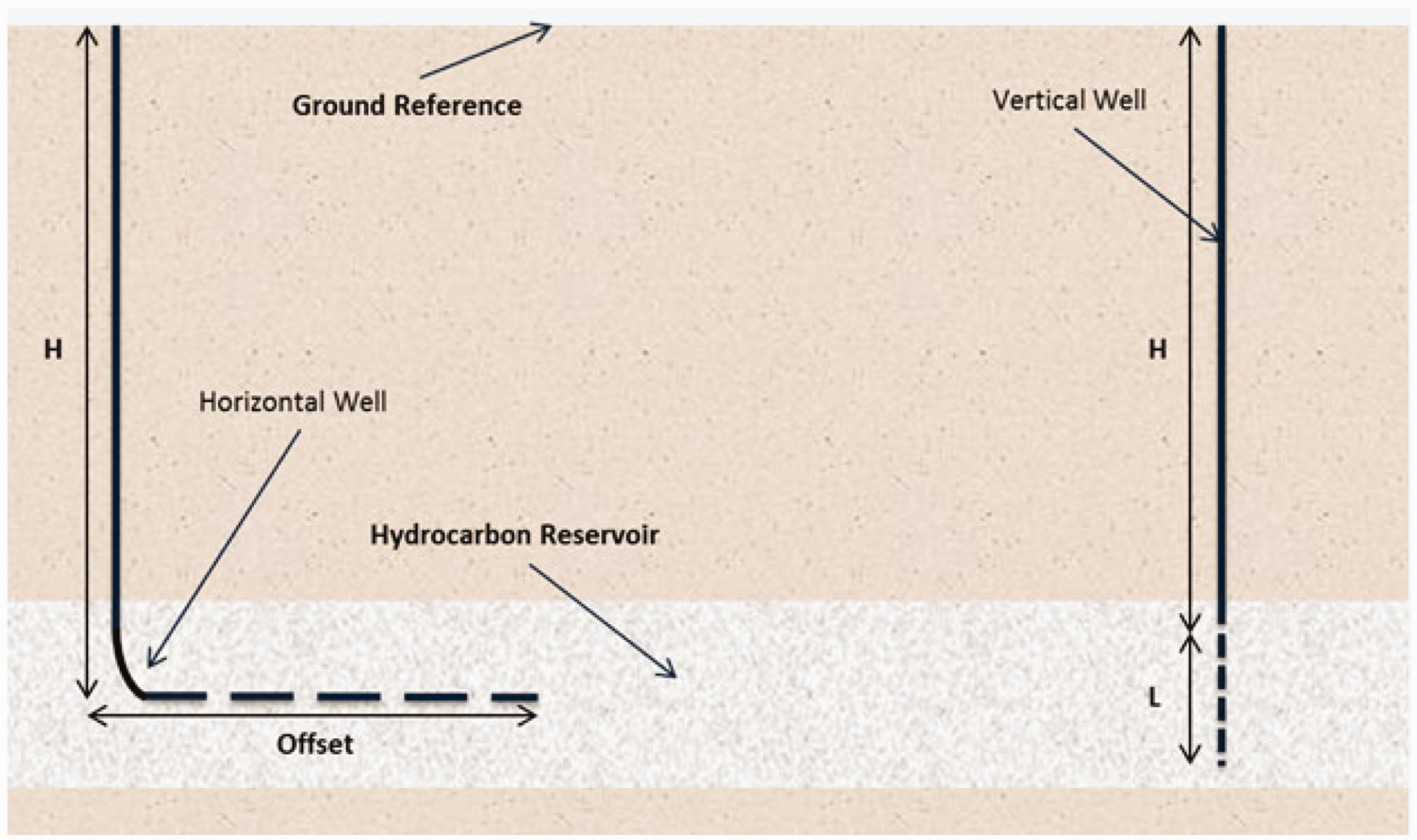
Horizontal well (left) and vertical (right) well penetrating a hydrocarbon reservoir.

By writing a Matlab code, the first step will be to determine the 10 variables (9 inputs and 1 output) characterising any well as indicated in Figure 1 with respect to a set of constraints that will be introduced in the following section. For this, the ANN will be added to the optimization process, and with respect to a maximum number of wells to drill, the algorithm will start to seek for places with higher oil saturation “S_o” to drill producers and places having a minor “S_o” to drill injectors. Hence, the simulation will generate at each iteration “t”, a well with all its relevant parameters (x, y, z, type, geometry, length or offset “L”, orientation angle “α” and total flow “Q_tot”) till the maximum specified number of wells is reached; then, things will be ready to estimate for each well, water-cut, near-wellbore pressure, near-wellbore water saturation; in addition to total liquid recovered from and injected into the reservoir.

After that, the second part of the job – carried out right after the first step in the same loop – will be dedicated to the determination and optimization of the trajectory of each well. What is meant by trajectory optimization is to get at small well length as possible which in turn will lead to low drillings costs. This task is achieved using a 3^rd order Bézier curves and will be shown later in detail. At the end of this process, the main outputs will consist of a complete deviation survey (North/South and East/West local coordinates, Vertical coordinates, measured depth (MD), inclination and azimuth), in addition the total well length and maximum dogleg severity.

Optimization problem formulation

Net-present value optimization

Objective function

The joint optimization of well placement and flow controls is a very challenging problem that put into play linear and non-linear constraints describing some considerations to satisfy with regards to well location, well trajectory (length and curvature as well), in addition to some production constraints and fluid handling capacity; all those for the sake of maximizing oil production with minimum water injection. Hence, selection of the best well location configuration is usually critical as it has a large consequence on investment and future reservoir performance. The optimization problem is going to be solved using a mixed-integer approach and the categorical variables (Well type and well geometry) were categorized using the “One-Hot Encoding” in order to turn them into numerical feature, as it is largely used when dealing with nominal variables.

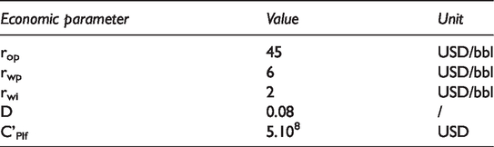
The widely used metric to assess the profitability from developing petroleum assets is termed as NPV which stands for net-present value. NPV is also useful when comparing different scenarios that involve different well configuration or different flow controls. The main goal in each time-step is to achieve a maximum NPV and the economic parameters that will be applied so are summarized in Table 1.

Table 1.

Inputs for the optimization of NPV.

Economic parameter	Value	Unit
rop	45	USD/bbl
rwp	6	USD/bbl
rwi	2	USD/bbl
D	0.08	/
C’Plf	5.108	USD

The joint optimization of flow control setting and well placement, given a set of linear and non-linear constraints, is commonly formulated for the sake of maximizing the net-present value of a hydrocarbon-bearing asset by the following equations objective functions:

$$\mathrm{NPV}=\sum _{\mathrm{j}=1}^{{\mathrm{N}}_{\mathrm{t}}}\left\{\frac{\left[\left({\sum }_{\mathrm{k}=1}^{{\mathrm{N}}_{\mathrm{p}}}{{\mathrm{r}}_{\mathrm{op}}\mathrm{Q}}_{\mathrm{op},\mathrm{k}}\left(\mathrm{t}\right)-{\sum }_{\mathrm{k}=1}^{{\mathrm{N}}_{\mathrm{p}}}{{\mathrm{r}}_{\mathrm{wp}}\mathrm{Q}}_{\mathrm{wp},\mathrm{k}}\left(\mathrm{t}\right)-{\sum }_{\mathrm{k}=1}^{{\mathrm{N}}_{\mathrm{i}}}{{\mathrm{r}}_{\mathrm{wi}}\mathrm{Q}}_{\mathrm{wi},\mathrm{k}}\left(\mathrm{t}\right)\right)-{{\mathrm{C}}^{\mathrm{\prime }}}_{\mathit{Plf}}-{{\mathrm{C}}^{\mathrm{\prime }}}_{DC,i}\left(\mathrm{t}\right)\right]*{\Delta \mathrm{t}}_{\mathrm{j}}}{{\left(1+\mathrm{D}\right)}^{\frac{{\mathrm{t}}_{\mathrm{j}}}{\mathrm{\tau }}}}\right\}$$

(1)

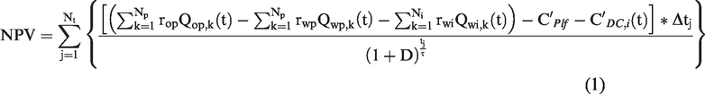
Where:

Q_op,_k: Oil production rate of well “k”.

Q_wp,_k: Water production rate of well “k”.

N_p: Total number of producers.

Q_wi,_k: Water injection rate of well “k”.

N_i: Total number of injectors.

C′_plf: Costs of mobilizing the drilling platform.

C′_DC: Costs of drilling and completing a Well “i”.

The costs of drilling and completing a well, denoted by “C′_DC”, were calculated based on vertical and horizontal offset of a well to its end point, respectively “Δz” and “Δxy”, using the following formula:

$${\mathrm{C}\mathrm{\prime }}_{\mathrm{DC},\mathrm{i}}=5000*\Delta \mathrm{z}+10000\left||\Delta xy\right|$$

(2)

Remark

Costs inherent to mobilize the drilling platform will be accounted at the 1st time-step only.

Drilling and completion costs will be considered only once each time a well is added to the drilling schedule.

Maximum duration to drill a well was set to three month.

The field is to be produced for 20 years and the flow settings are to be updated quarterly, thus the total number of time-step intervals (iteration) to carry out the whole simulation will be 80 time-steps.

A producer will be shut in if its water cut goes beyond 90%.

Constraints formulation

In order to have a comprehensive field development strategy and a detailed drilling schedule, it is fundamental to formulate any optimization problem by stating some hypotheses and taking into consideration technical constraints with respect to acceptable well engineering practices.

Firstly, we chose to operate each well quarterly, hence each 3 month we will have an updated flow allocation for any injector or producer in addition to the other well parameters location indicated in Figure 1.

Since the reservoir is located offshore, all the wells will have the same starting point and only monobore configuration will be considered for each well (neither fishbone nor multilateral configuration was taken into account).

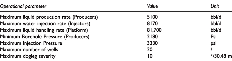
From an operational standpoint, any well should be operated within some limits initially set based on well, flowlines and surface facilities technical design and limitations. Table 2 summarizes the operational constraints that were retained for this exercise.

Table 2.

Summary of operational constraints.

Operational parameter	Value	Unit
Maximum liquid production rate (Producers)	5100	bbl/d
Maximum water injection rate (Injectors)	8170	bbl/d
Maximum liquid handling rate (Platform)	81,700	bbl/d
Minimum Borehole Pressure (Producers)	2180	Psi
Maximum Injection Pressure	3330	psi
Maximum number of wells	20	/
Maximum dogleg severity	10	°/30.48 m

Moreover, well implantation problem is usually formulated by different linear and non-linear constraints. Below is a summary of all constraints that were applied during the sequential optimization of well placement and well total length.

Geometric limits

This is to ensure that the algorithm will set the segment in contact with the reservoir, at a location comprised between the top and the bottom of the reservoir, and also to ensure that the start point “S” and end point “E” of that segment will be set within the contours of the reservoir.

- Vertical well

$${\mathrm{Z}}_{\mathrm{top}}\le {\mathrm{z}}_S\le {\mathrm{Z}}_{\mathrm{bot}}$$

(3)

$${\mathrm{Z}}_{\mathrm{top}}\le {\mathrm{z}}_E\le {\mathrm{Z}}_{\mathrm{bot}}$$

(4)

- Horizontal well

$${\mathrm{x}}_{\min }\le \left\{x_S,x_E\right\}\le {\mathrm{x}}_{\max }$$

(5)

$${\mathrm{y}}_{\min }\le \left\{y_S,y_E\right\}\le {\mathrm{y}}_{\max }$$

(6)

In equations (5) and (6), “x_E” and “y_E” will be expressed as function of “x_S” and “y_s” respectively, and also as function of the length of the segment “L” – penetrating the reservoir – and well orientation “α” (Figure 4), as follows:

$${\mathrm{x}}_{\mathrm{E}}={\mathrm{x}}_{\mathrm{S}}+\mathrm{L}\times \cos \left(\mathrm{\alpha }\right)$$

(7)

$${\mathrm{y}}_{\mathrm{E}}={\mathrm{y}}_{\mathrm{S}}+\mathrm{L}\times \sin \left(\mathrm{\alpha }\right)$$

(8)

Figure 4.

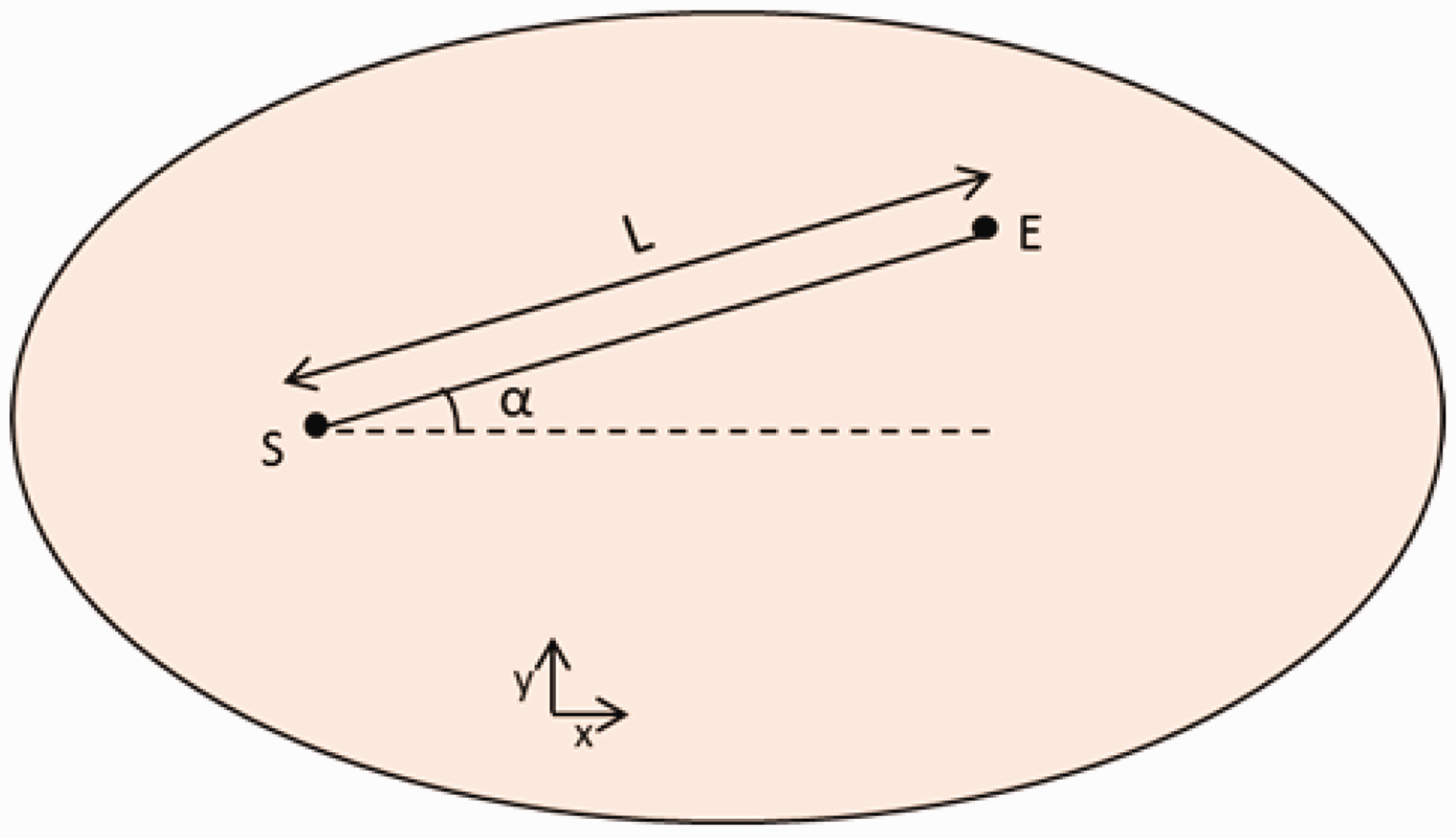
Planar view of a horizontal well penetrating a reservoir.

Minimum well distance

A minimum well distance criterion was considered based on different values found in the literature. For any new well to be positioned in the reservoir, the minimum distance should not exceed 800 m. This constraint was formulated to take into account the segment penetrating the reservoir. Each segment is represented by two points and the minimum distance between two segments is defined by the shortest distance between these segments. A lot of theories can be found in the literature to get the shortest distance between two segments. In this work, the calculation of the minimum distance was carried out using a built-in function available in the Matlab environment.

Drilling and completion duration “T_DC”

Each well should be drilled and completed in a duration that does not exceed 90 days.

$${\mathrm{T}}_{\mathrm{DC}}=0.015\times \Delta \mathrm{z}+0.02\times \left|\Delta xy\right|<90\hspace{0.17em}\mathrm{days}$$

(9)

Initial water saturation “s_wi”

From an economic point of view, a producer has to be placed in a location wherein the initial water saturation “S_wi” is less than 0.4 (or initial oil saturation “S_oi” up to 0.4). This is to have as maximum oil volumes in place as possible. For an injector, it was decided to implant potential wells in places where smaller oil volumes exist, with the intention of sweeping those volumes to locations where producers are already operational.

Producer well:

$${\mathrm{S}}_{\mathrm{w},\mathrm{init}}<0.4$$

(10)

Injector well:

$${\mathrm{S}}_{\mathrm{w},\mathrm{init}}>0.7$$

(11)

Constraints handling

For the purpose of constraints handling, three feasibility rules methodology will be used to solve the flow allocation and well placement problem. These rules were implemented in the GA optimizer by considering a liner ranking criterion for the estimation of the objective function. The feasibility rules methodology can be described according to the following set of priorities:

Feasible solutions will be prioritized over non-feasible ones.

For the case feasible solutions, the ones that yield higher values of objective function will be favored over the ones yielding lower values.

In the case of non-feasible solutions, the ones that violate the constraints less will be prioritized.

Concerning nonlinear constraints,

Well trajectory optimization

Well trajectory optimization is generally formulated such that for any well planned for a future drilling, well length and curvature will be optimized. While reducing the length will have a significant impact on reducing drilling costs, minimizing dogleg severity will help getting smooth wells trajectories, hence allowing steerable deviation tools to operate at favourable conditions and avoid an unwanted downturn in drilling activities or sudden downhole accidents.

Therefore, wells trajectories will be optimized with respect to a maximum dogleg using 3rd order Bézier curves method. This method is fairly easy to apply especially when it has to do with designing three-dimensional complex well trajectories. In addition, the flexibility of using 3rd order Bézier curves in comparison to some other methods (cubic functions, double arc, constant curvature, etc.) is that they allow the determination of a well path with the aid of a one single equation that handles the three spatial coordinates all at once. The next subsection is an illustration of how to determine well trajectories using the 3rd order Bézier curves.

Well path design using 3rd order Bézier curves

3rd order Bézier curves, as illustrated by Figure 5, are parametric curves defined according to the following general expression that is applied for the case of a “Set-End” trajectory, i.e., the case in which the azimuth and inclination are set and have to be met:

$$\text{B}\left(\text{u}\right)\text{ = }{\left(\text{1-u}\right)}^{\text{3}}\text{S+3}{\left(\text{1-u}\right)}^{\text{2}}\text{u}{\text{C}}_{\text{Sp}}\text{+3}\left(\text{1-u}\right){\text{u}}^{\text{2}}{\text{C}}_{\text{Ep}}\text{+}{\text{u}}^{\text{3}}\text{E}$$

(12)

Figure 5.

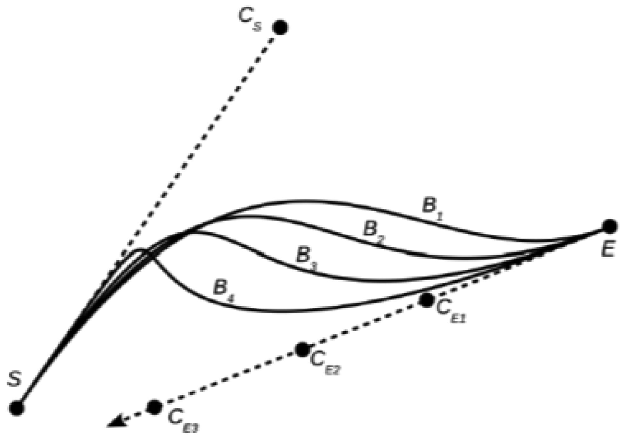
Illustration of a 3rd order Bézier curve.

The position of attractor “C_Sp” – located at some distance ahead of the starting point “S”– and the other attractor “C_Ep” – located at some certain distance behind of the ending point “E”– are respectively calculated as function of a unit tangent vector Tt”, and a scalar parameter “d” that controls the shape of well path:

$${\text{C}}_{\text{Sp}}\text{ = S + }{\text{d}}_{\text{Sp}}{\text{T}}_{\text{Sp}}$$

(13)

$${\text{C}}_{\text{Ep}}\text{ = E + }{\text{d}}_{\text{Ep}}{\text{T}}_{\text{Ep}}$$

(14)

Here again, the unit tangent vectors “T_Sp” and “T_Ep” are function of inclination “θ” and azimuth “φ”, and usually defined based on three components as follows:

$${\text{T}}_{\text{Sp}}\text{ = (}\text{cos}{\text{θ}}_{\text{S}}\text{, sin}{\text{θ}}_{\text{S}}\text{cos}{\text{φ}}_{\text{S}}\text{, sin}{\text{θ}}_{\text{S}}\text{sin}{\text{φ}}_{\text{S}}\text{)}$$

(15)

$${\text{T}}_{\text{Ep}}\text{ = (}\text{cos}{\text{θ}}_{\text{E}}\text{, sin}{\text{θ}}_{\text{E}}\text{cos}{\text{φ}}_{\text{E}}\text{, sin}{\text{θ}}_{\text{E}}\text{sin}{\text{φ}}_{\text{E}}\text{)}$$

(16)

Now that all the critical parameters of the Bézier equations are known, it is possible now to proceed to the determination of the trajectory length, i.e., total well length.

Length of a well trajectory

Several expressions were proposed in order to determine the trajectory length, but for practical reasons, the following approximation will be used:

$$\mathrm{L}\left({\mathrm{u}}_{\mathrm{i}}\right)=\sum _1^{\mathrm{i}}\frac{{\mathrm{\gamma }}_{\mathrm{i}}}{\sin {(\mathrm{\gamma }}_{\mathrm{i}})}{\mathrm{\Delta }\mathrm{L}}_{\mathrm{i}}$$

(17)

Where:

$${\text{ΔL}}_{\text{i }}\text{= }\sum _{\text{1}}^{\text{i}}\left[\sqrt{{\left(\mathrm{\Delta }{\mathrm{v}}_{\mathrm{i}}\right)}^2+{\left(\mathrm{\Delta }{\mathrm{n}}_{\mathrm{i}}\right)}^2+{\left(\mathrm{\Delta }{\mathrm{e}}_{\mathrm{i}}\right)}^2}\right]$$

(18)

$${\text{γ}}_{\text{i}}\text{ = arcos}\left[\mathrm{t}\left({\mathrm{u}}_{\mathrm{i}}\right)*\mathrm{t}\left({\mathrm{u}}_{\mathrm{i}-1}\right)\right]$$

(19)

Dogleg severity “DLS”

$$\overrightarrow{\mathrm{k}}=\frac{\ddot{\mathrm{B}}}{\dot{\mathrm{B}}*\dot{\mathrm{B}}}-\frac{\dot{\mathrm{B}}*\ddot{\mathrm{B}}}{{\left(\dot{\mathrm{B}}*\dot{\mathrm{B}}\right)}^2}*\dot{\mathrm{B}}$$

(20)

The first and second derivatives of function “B” with respect to the variable “u” are as follows:

$$\dot{\mathrm{B}}\left(\text{u}\right)\text{ = }{-3\left(\text{1-u}\right)}^{\text{2}}\text{S+3}\left(\text{1-u}\right)\left(\text{1-3u}\right){\text{C}}_{\text{Sp}}\text{\hspace{0.17em}+\hspace{0.17em}3}\left(\text{2-3u}\right)\text{u}{\text{C}}_{\text{Ep}}+{\text{3u}}^{\text{2}}\text{E}$$

(21)

$$\ddot{\mathrm{B}}\left(\text{u}\right)=\text{6}\left(\text{1-u}\right)\text{S\hspace{0.17em}-\hspace{0.17em}6}\left(\text{2-3u}\right){\text{C}}_{\text{Sp}}+\text{6}\left(\text{1-3u}\right){\text{C}}_{\text{Ep}}+\text{6uE}$$

(22)

From the above equation, the dogleg severity “DLS” is simply the module of the vector “k” expressed in “°/30.48 m”.

$$\mathrm{DLS}=30.48*‖\overrightarrow{\mathrm{k}}‖$$

(23)

In conclusion of this subsection, a full procedure along with some examples was addressed by Sampaio (2017) to determine all the aforementioned parameters.

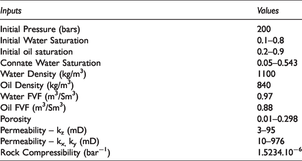
Reservoir model description

The model that we aim to investigate throughout this paper is a virtual single layer dynamic reservoir model representing an offshore oil field originally built upon data gathered from 7 exploration wells. The dynamic model – as per initial development plan – was generated based on 16 wells (i.e., 10 producers and 6 injectors), it was decided to study the option and investigate the economic viability of having 20 wells (14 producers and 6 injectors) under operation with a focus on water injection as a means of oil recovery enhancement, and to pinpoint the outcomes of this strategy in comparison to the initial plan built upon 16 wells.

The reservoir in question is a single layer sandstone reservoir with a lot of thin shale layers. The porosity and the different permeabilities of this reservoir were generated following a normal distribution. The vertical permeability is set as tenth of the horizontal permeability. The top of the reservoir is situated at 2100 m depth, and the primary evaluations reported 330 million oil barrels in place. Initial logging measurements indicated that the initial pressure is nearly 200 bars and the initial water saturation is the range of 0.1–0.8. The dynamic model was defined over a 150 × 150 × 16 simulation grid, each of which has a 200 m × 200 m × 10 m spatial dimensions. Some of the data that were used during the optimizations are summarized in Table 3.

Table 3.

Reservoir parameters used during the optimization process.

Inputs	Values
Initial Pressure (bars)	200
Initial Water Saturation	0.1–0.8
Initial oil saturation	0.2–0.9
Connate Water Saturation	0.05–0.543
Water Density (kg/m3)	1100
Oil Density (kg/m3)	840
Water FVF (m3/Sm3)	0.97
Oil FVF (m3/Sm3)	0.88
Porosity	0.01–0.298
Permeability – kz (mD)	3–95
Permeability – kx, ky (mD)	10–976
Rock Compressibility (bar−1)	1.5234.10−6

Results summary

Proxy model performance

As stated earlier, a spatiotemporal dataset comprised of all the variables presented in Figure 1, was generated from a set of data taken out from reservoir simulation results.

After encoding the categorical features using the “One-Hot Encoding” method, we proceeded to the elimination of outliers using the “Quartiles” rule. Then, the dataset was split into training and validation data using the 70/30 percent rule, then a deep learning process was applied to those data using a very promising type of neural network called Radial basis Neural Networks (RBNN) because of their easy design, good generalization and smaller extrapolation errors.

Table 4 show the some parameters that were used during the neural network learning process along with some metrics. A regularization process was also applied to improve generalization and avoid overfitting. This generally involves modifying the performance function, i.e. the mean sum of squares error (MSE), generally used during the training process.

Table 4.

RBNN modelling – parameters and metrics.

Parameter	Value
Regularization
Epoch	300
Goal	1e-5
Regularization	0.5
RBNN
MSE (Goal)	2
Spread	5
Prediction Model – Metrics
MSE (Achieved)	1.845
R2	0.99987
Total Neurons	750

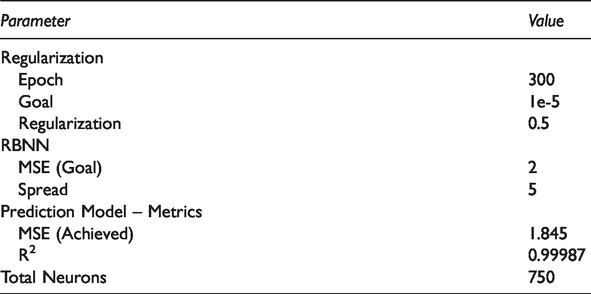
From Table 4, we can conclude that the RBNN approach used to set the reservoir proxy model is able to yield good responses to the target variable, i.e. bottom-hole pressures, with high accuracy (R² = 0.99987). This fact can be checked from Figure 6 (left). The boxplot illustrated by Figure 6 (right) summarises some statistics expressed as error fractions of BHP raw data. Despite the presence of some outliers, it is noteworthy to mention that the maximum error observed through the learning process is about 0.003505 (nearly 0.35%), while the median of those error fractions is 0.00051413 (0.052%). The same findings were reported by Nwachukwu et al. (2018a, 2018b) concerning the presence of outliers in the error fractions histogram, and this does not seem to interfere with overall prediction performance of proxy model.

Figure 6.

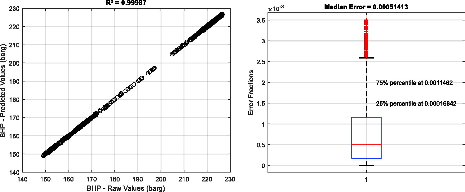
Predicted BHP vs Raw BHP (left). Boxplot of error fractions (right).

Production performance

In this section, the different results that were obtained after carrying out several runs on the optimization strategy will be presented. Firstly, a comparison will be made in terms of NPV, field total oil production “FTOP”, field total water production “FTWP” and field total water total injection “FTWI” between different scenarios over a 20-year period.

Table 4 shows the main results regarding 4 scenarios that we have taken into consideration. These scenarios represent several development strategies which are defined as follows:

Scenario “1” (Base case): 10 producers and 6 injectors operated at their maximum operational limits.

Scenario “2”: Optimization of scenario “1” (10 producers and 6 injectors) based on the operational constraints defined in Table 2.

Scenario “3”: Joint optimization of flow allocation and well placement of the base case defined by scenario “1” considering all the constraints defined in section III.1.2 and III.2.2.

Scenario “4”: Joint optimization of flow allocation and well placement considering 14 producers and 6 injectors.

As can be seen from Table 5, the net increase in oil production and NPV when comparing scenarios “1” and “2” can be attributed the reduction of water breakthrough as a consequence of choking back the 6 injectors. Indeed, the decrease of total water injection has resulted in the decrease of water production as well over the 20-year whole field life-cycle, and the overall oil production has gone up from 74.15 MM STB to approximately 102.5 MM STB.

Table 5.

Outcomes of different development strategy over the field’s life-cycle.

Scenario	NPV (MM $)	FTOP (MM STB)	FTWP (MM STB)	FTWI (MM STB)
Scenario “1”	1455.906	74.146	206.145	285.682
Scenario “2”	3265.053	102.542	182.221	278.731
Scenario “3”	3479.821	205.423	13.263	114.315
Scenario “4”	4351.020	258.311	12.829	130.394

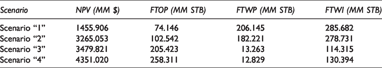
It appears also from the joint optimization strategy (Scenario “3”) applied on the base case has shown - in comparison to scenarios “1” and “2” – a noticeable increase in oil production volumes and a net decrease in water injection and water production. This can be attributed to wells being positioned in profitable locations that favour maximum oil recovery and lower water production. With regards to scenario “4”, the joint optimization of well placement and flow settings of 20 wells (14 producers and 6 injectors) could allow to achieve a higher NPV (4.351 billion USD) and a higher total oil production (258.3 million STB) than the other scenarios. Compared to scenario “1”, the field development strategy applied according to scenario “4” is much likely to improve NPV by 3 folds with some noticeable expenses due to water injection.

Production and injection rates of scenario “4” are sketched in Figure 7. Over the years, wells got drilled and field liquid production rate increases, while water injection starts from year 3.75 after the first injector, i.e. Well 15, is drilled and completed (see Table 6). The sudden increase in liquid production rate from year 5 could be attributed to the number of constraints that our optimization code deals with. The drilling schedule extends from year 0 to year 5 and along this period, the algorithm deals with more than 15 linear and non-linear constraints and a total of 10–48 variables. After that, the optimization will consist in setting the flowrates and their corresponding wellbore pressures from year 5 to year 20. Since the FDP was established to drill 20 wells, we will end up with 40 variables and only one linear constraint to deal with which is the platform liquid handling capacity (Table 2).

Figure 7.

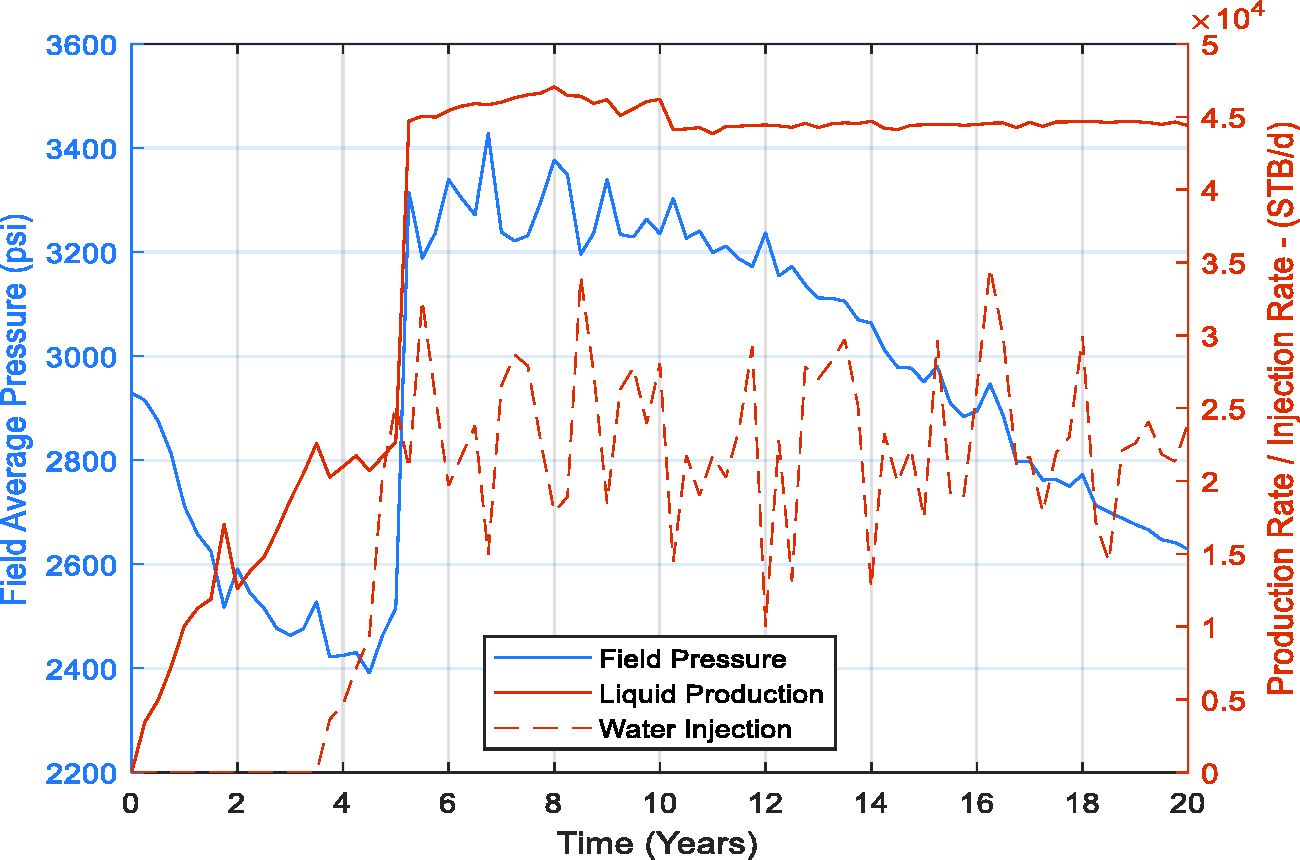
Average reservoir pressure versus production/injection rates.

Figure 8.

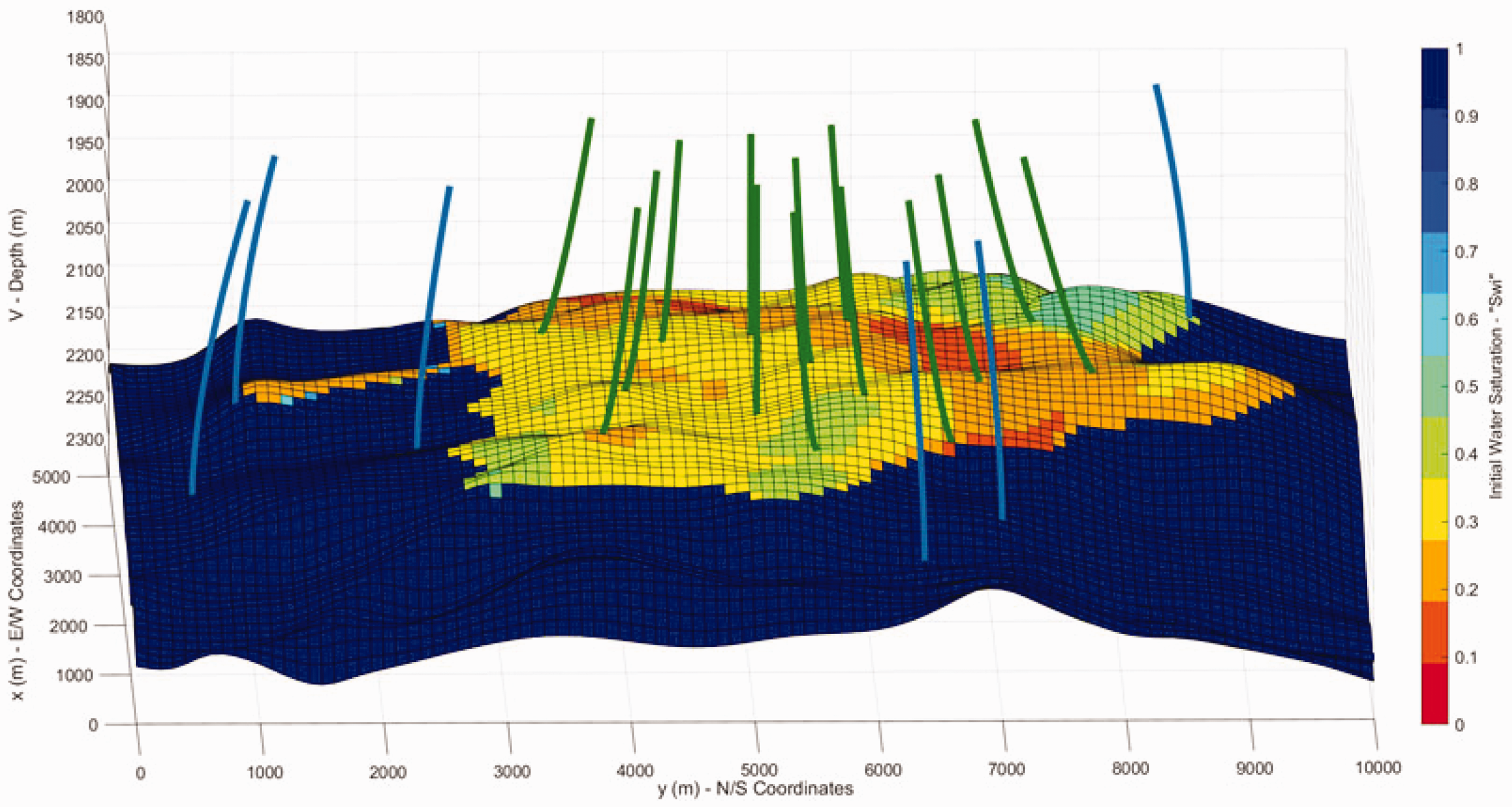
Well locations in the reservoir (Green lines: Producers – Blue lines: Injectors).

Table 6.

Drilling schedule.

Well	t (years)	Location			Type	Geometry	Length (m)	α
		x (m)	y (m)	z (m)
1	0	5106.1	2521.7	2076.7	Producer	Vertical	15	0
2	0.25	6381.7	2164.5	2063.5	Producer	Horizontal	351	99.2
3	0.5	4091.5	2988.7	2088.9	Producer	Horizontal	385	119.9
4	0.75	4747.0	1675.9	2087.0	Producer	Horizontal	248	274.9
5	1	7915.9	2672.1	2070.9	Producer	Horizontal	414	165.7
6	1.25	3007.6	4266.5	2084.1	Producer	Horizontal	236	246.9
7	1.5	3803.8	1185.2	2087.8	Producer	Horizontal	354	160.9
8	1.75	4926.5	3649.7	2060.1	Producer	Horizontal	283	258.4
9	2	8083.6	3910.6	2084.4	Producer	Horizontal	483	292.0
10	2.25	6855.4	3473.2	2083.8	Producer	Horizontal	300	245.9
11	2.5	3546.8	2328.0	2088.9	Producer	Horizontal	186	149.2
12	2.75	1233.4	3118.1	2087.2	Producer	Horizontal	107	161.9
13	3	5919.4	3240.0	2056.4	Producer	Horizontal	248	222.2
14	3.25	2085.5	3406.3	2090.9	Producer	Horizontal	92	193.6
15	3.5	2072.2	2394.3	2127.0	Injector	Vertical	10	0
16	3.75	6378.4	667.1	2142.2	Injector	Vertical	14	0
17	4	1826.5	1484.7	2108.0	Injector	Vertical	12	0
18	4.25	1063.3	1844.4	2124.6	Injector	Vertical	11	0
19	4.5	8707.7	1692.4	2149.4	Injector	Vertical	10	0
20	4.75	9133.2	4473.1	2134.5	Injector	Vertical	21	0

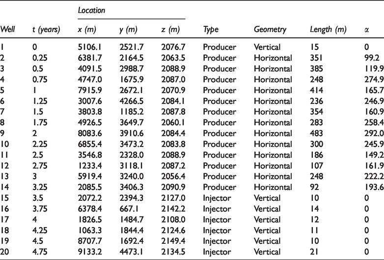
Drilling schedule and well placement

The drilling schedule generated by our Matlab code at the end of the joint optimization simulations is summarized in Table 6. Some guidelines were set in order to favour the drilling of producers before injectors. This was intentionally favoured in order to maximize revenue at early stages of the life-cycle of offshore oilfield. It is to mention that the drilling plan will consist in drilling 7 vertical wells - 1 producer (Well 1) and 6 injectors (Wells 15 to 20), and 13 horizontal wells which are all producers.

Drilling and completion overall activities will be theoretically achieved in almost 5 years and all these wells were implanted in preferred locations. Table 7 illustrates the length, maximum dogleg, initial water saturation, drilling and completion duration and costs (costs were estimated using equation (2)) for each well. All the constraints that were listed in Table 1 and defined in equations (3) through (11) were honoured. Regarding wells’ production (or injection) performances, a summary of flow allocation and wellbore pressure settings for some producers and injectors can be checked in Appendix 1.

Table 7.

Wells’ characteristics.

Well	Total length (m)	Max Dogleg (°/30.48m)	Swi	Drilling and completion
				Duration (days)	Costs (MM $)
1	2091.7	0	0.283	31.4	10.46
2	3062.7	6.21	0.275	36.2	22.51
3	3048.4	7.32	0.299	37.1	24.93
4	2813.5	5.32	0.338	35.0	21.88
5	4008.1	5.35	0.385	37.3	34.57
6	4069.0	7.91	0.313	34.8	37.13
7	3511.3	9.92	0.342	36.6	30.86
8	2805.5	5.05	0.398	35.1	19.13
9	4926.1	5.75	0.389	38.5	43.38
10	3372.2	9.49	0.400	35.8	28.04
11	3119.7	9.61	0.395	34.1	27.66
12	5089.8	6.76	0.400	32.9	50.68
13	2745.8	4.91	0.391	34.6	18.65
14	4339.9	8.34	0.489	32.7	42.73
15	4151.9	8.83	0.998	32.1	41.05
16	3479.0	5.70	0.997	32.3	33.27
17	4536.4	5.22	0.985	31.8	45.00
18	5185.2	7.10	0.997	32.0	51.67
19	4809.2	5.82	0.997	32.4	47.76
20	5581.5	8.14	1	32.3	55.53

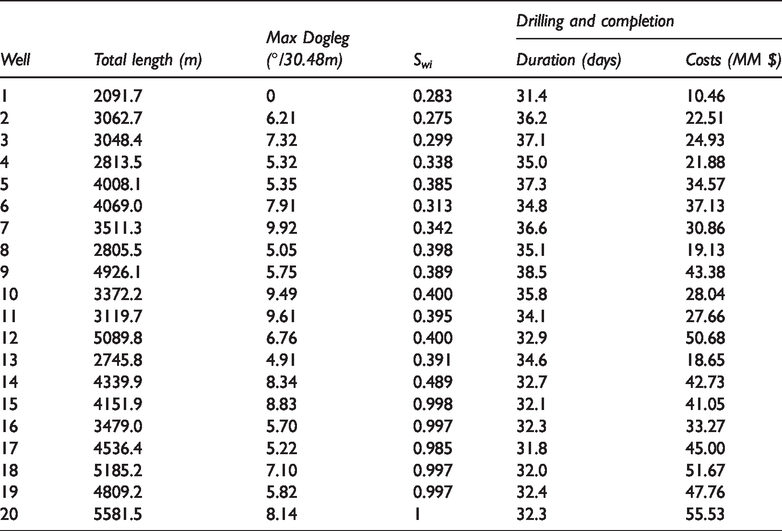
The producers were placed in locations wherein “S_wi” is less than 0.4 in order to get maximum oil volumes, except well “14” which was placed in a location having a “S_wi” equal to 0.489. This does not seem to have a significant impact on well performance. On the other hand, the injectors were set in water-bearing zones, i.e., places having “S_wi” up to 0.7 for pressure support (Figure 8). These facts are enough proof to say that our Matlab code is able to find feasible solutions that satisfy the conditions that were imposed on the optimizer. In addition, drilling and completing all the wells could be achieved in a time less than 39 days and the maximum dogleg for all the wells is below 10°/30.48 m. A full deviation survey of some vertical and horizontal wells that were identified to develop the oil field can be examined in Appendix 2 (Tables 8 and 9). It is noteworthy to mention that all the deviation surveys were determined by implementing a Matlab script based on equations (12) through (23) and the trajectory of every well is illustrated in Appendix 3.

Conclusion

The joint optimization of flow control, well placement, and well length is a tough and very challenging exercise that petroleum reservoir specialists and decision-makers need to establish and determine in order to get a full idea on reservoir performance over its life-cycle as well as investment and return on investments. The objective was to propose a genuine approach for the joint optimization of well placement, well path design and production/injection allocation, in addition to a well drilling schedule as part of a field development plan strategy, and it appeared that genetic algorithms are robust tools for solving a mixed integer optimization problem constrained by a set of linear and non-linear constraints.

The proposed optimization strategy was carried out in order to get optimal well locations and as much oil volumes as possible to recover. This challenge was performed by implementing a Matlab code and several constraints were formulated in order to achieve the objectives of this study. A lot of scenarios were investigated and it appeared that the scenario we have chosen to develop the investigated offshore oil field is very likely to yield massive net-present value with respect to maximum operational capacity of wells to deliver liquids and the platform to handle the delivered oil and water volumes. In addition, the algorithm that we developed was able to position the producers and injectors in desired locations depending on local water saturations, and clear drilling schedule was established along with the maximum duration for each well to be spudded and completed so that the operators can have at hand an overview on the drilling timeline to follow in order for them to set the financial and technical means regarding the accomplishment of drilling and completion activities. Moreover, a full deviation survey of each well was also delivered to serve as a guideline and the well trajectories were designed in order to get smooth well paths. This characteristic is critical as it ensures easier access to wellbore during subsequent interventions such as stimulation or wireline jobs in addition to potential work-over jobs.

In continuation to this study, future works will consist of using our Matlab code to more complex hydrocarbon fields by considering multi-layered reservoirs, multi hydrocarbon traps as well as integrating geologic features such as fault. The problematic of geologic and economic uncertainty will be also taken into account, and we will try to incorporate additional details of the hydrocarbon chain, such as the operational limits of the processing facility and pipelines. Nevertheless, a primary focus will be put on the enhancement of the approach adopted in this work and the validation of our code. The reservoir parameters, the optimized well locations and trajectories and the all constraints that were addressed earlier will be fed into a commercial reservoir simulator in order to see how the findings that were presented herein match with the results that could be obtained through reservoir simulation.