Sage Journals: Discover world-class research

Abstract

Lead–acid battery is the common energy source to support the electric vehicles. During the use of the battery, we need to know when the battery needs to be replaced with the new one. In this research, we proposed a prediction method for voltage and lifetime of lead–acid battery. The prediction models were formed by three kinds mode of four-points consecutive voltage and time index.The first mode was formed by four fixed voltages value during four weeks, namely M1. The second mode was formed by four previous voltage values from prediction time, namely M2. Third mode was formed by the combinations of four previous data with the last predicted data, namely M3. The training data were recorded from 10 lead–acid batteries. We separated between training data and testing data. Data collection for training were recorded in 155 weeks. The examined data for the model was captured in 105 weeks. Three of batteries were selected for prediction. Machine learning methods were used to create the batteries model of voltage and lifetime prediction. Convolutional Neural Network was selected to train and predict the battery model. To compare our model performance, we also performed Multilayer Perceptron with the same data procedure. Based on experiment, M1 model did not achieve the correct prediction besides the linear case. M2 model successfully predicted the battery voltage and lifetime. The M2 curve was almost the same with real-time measurement, but the curve was not fitting smoothly. M3 model achieved the high prediction with smooth curve. According to our research on lead–acid battery voltage prediction, we give the following conclusions and suggestions to be considered. The accuracy of prediction is affected by the number of input parameters is used in prediction. The input parameters need to have time consecutive.

Keywords

Lead–acid battery life cycle Convolutional Neural Network multilayer perceptron

Introduction

Since the battery was invented, more and more devices have become stand-alone devices that can be carried around (Elliott, 1999; Kurzweil, 2010; Whittingham, 1976). After some days, everyone realized that the use of the battery needs to be managed because of some unexpected events, so the battery management system (BMS) (Liu et al., 2019) or the energy management system (Homan et al., 2019) was developed. Effective management can extend the life and prevent the battery from failing during use. Since the main components of a battery are composed of chemical elements and store electrical energy, there are many unstable elements. Therefore, the conditions of use and storage will directly affect the performance of the battery.

As of today, common rechargeable batteries are lead–acid battery series and lithium-ion battery series. The earliest lead–acid batteries and lithium-ion batteries were proposed in 1859 (Kurzweil, 2010) and 1976 (Whittingham, 1976), respectively. In the past records, lithium-ion batteries have caused many explosions due to improper use and improper circuit design, which has led to the emergence of BMSs (Liu et al., 2019). Lithium-ion batteries have been able to provide considerable control and protection in the state-of-the-art design of BMS (Ali et al., 2019). The parameters in these designs are calculated and controlled based on real-time data. Although the battery’s instability is limited, it is not enough to match the actual design to the battery’s performance. As a result, more and more research results have begun to use data science rather than traditional numerical analysis in the past. An excellent study in this field is to estimate and predict the health and life cycle of batteries (Hinchi and Tkiouat, 2018; Khumprom and Yodo, 2019; Laayouj and Jamouli, 2015; Li et al., 2016; Liu et al., 2010; Ren et al., 2018; Zhang et al., 2018).

Battery life cycle prediction uses numerical methods such as data-driven support vector machines (SVM) or Gaussian process regression in the early days (Laayouj and Jamouli, 2015; Li et al., 2016). However, these methods still do not fully describe the nonlinear battery characteristic curve, so the combination of these methods makes it more complete. The evolution of data science, machine learning is used in battery data analysis. Some data features are periodic, some have specific amplitudes, and some have specific conditions. This is a considerable challenge in the past, but machine learning can easily solve these problems. long short term memory (LSTM) and Recurrent Neural Network (RNN) are often used in timing-related parameter analysis (Hinchi and Tkiouat, 2018; Liu et al., 2010; Zhang et al., 2018). Deep Neural Networks (DNN) analyses more parameters with more complex variables (Khumprom and Yodo, 2019; Ren et al., 2018).

The invention of lead–acid batteries is about 100 years earlier than lithium-ion batteries, but many studies and designs have been published for research on lithium-ion batteries, and there are many opportunities for research on lead–acid batteries (Lyu et al., 2017; Wibawa et al., 2017). However, the interesting thing is that most of the vehicle applications are still dominated by lead–acid batteries. Therefore, we reviewed the related prediction techniques for lithium-ion batteries (Hinchi and Tkiouat, 2018; Khumprom and Yodo, 2019; Laayouj and Jamouli, 2015; Li et al., 2016; Liu et al., 2010; Ren et al., 2018; Zhang et al., 2018) and the literature on machine learning for battery life prediction (Álvarez Antón et al., 2013; Berecibar, 2019; Chaoui et al., 2017; Rezvani et al., 2011 ; Salameh et al., 2017; Zhang et al., 2017).

Machine learning is an artificial neural network (ANN) based data analysis method. The design of ANN is based on learning human brain neural activity. The purpose is to copy and learn human learning or thinking behavior patterns through this network. The main part of the neural network consists of the input layer, the hidden layer, and the output layer. The hidden layer is often composed of many different units, which convert the output data from the input layer into the output layer as the input. Although neural networks are composed of neural components that mimic humans, such mathematical model procedures are still too complex for humans (Alanis, 2018; Marcel and Sander, 2017; McCulloch and Pitts, 1943). ANNs have been developed since the 1940s, but it has only become a major part of artificial intelligence until recently. This is due to the recent development of a technique called Back Propagation that allows the network’s results to adjust its hidden neuron layer when it does not match the expected result. This major technological development has completely made the ANN have modified characteristics and more in line with the needs of artificial intelligence. Today’s ANNs have evolved many different learning models, such as the Convolutional Neural Network (CNN), RNN, DNN, Multilayer Perceptron (MLP), and SVM. Although a variety of neural network models are derived from mimic humans, they are actually used for different purposes.

MLP is one of the types of Forward Propagation Neural Networks. The design of the MLP includes at least three layers of nodes: the input layer, the hidden layer, and the output layer. It can also be composed of layers of more nonlinear active nodes. Since the MLP is fully connected, each node in the layer is connected to each node in the next layer with a certain weight. The MLP can be trained in supervised learning. The training process must reversely train the weights in a backward propagation manner so that the numerical values of the weights can be trained and updated to become supervised learning. MLP is similar to linear perceptron, but more layers and the use of nonlinear activation functions make a difference, and MLP can be used to separate data that cannot be linearly separated (Chien et al., 2018; Lin et al., 2018; Xiang et al., 2018).

CNN is a kind of DNN in deep learning. Because this network can solve large matrix problems, it is also often used to analyze visual images. CNN’s neural structure design is an MLP-based extended advanced design. Since the front-end convolutional layer and the pooling layer can achieve feature processing and data sampling, the input can be minimized. Inside the convolutional layer, there is no change in space and structure because of the sub-sampling layer and pooling design, so it is called Shift Invariant or Space Invariant Artificial Neural Network (Isogawa et al., 2018; Liang et al., 2018; Zhang et al., 2019). CNN can be seen as a bionic network architecture, a method derived from the imaging concept of animal visual nerves; the process by which the animal receives the image data and learns and then recognizes. Since the visual field that each optic nerve can sense is limited, there is an overlapping common field of view between the neurons, which allows the visual field sensed by each optic nerve to cover the range seen by the eyeball, and then sensed by the brain. The complete image transmitted by the optic nerve is recognized.

The lead–acid battery is still commonly used in electric vehicle. In production activity, it is necessary to know when the battery has to be replaced with the new one. For example, in heavy-duty trucks, the maintenance should be done regularly to avoid the unexpected failure because of the battery (Voronov et al., 2018). Some cases showed that the battery level degrades over repeated over-charge and over-discharge, especially for Lithium battery. It will reduce the lifetime of the battery quickly than it should be (Song et al., 2019). Usually, the operator just used the lead–acid battery without being maintained. In order to anticipate the problem, it is necessary to predict the lead–acid battery lifetime in real-time based on the open-circuit. A smart system is needed to estimate the lifetime of lead–acid battery based on the daily activity.

We can see that the current data forecasting technology, machine learning, and deep learning are becoming more and more mature. These technologies can be used to predict future data through a large amount of historical data. So, we propose a framework to apply these proven methods for lithium-ion battery applications to lead–acid battery systems. Since the condition of each battery is not the same, the conventional method is not suitable for use on every battery. Therefore, through the prediction technology, a voltage prediction model suitable for the battery can be established, so that information about the use condition or the life of the battery or an appropriate warning can be provided to prevent the battery from failing in operation.

The major contributions of this paper include the following:

Three methods for inputting data into the model are proposed, and the input method with both actual data and predicted data is the best.

The machine learning model for predicting the voltage of a lead–acid battery is established using CNN and MLP.

The rest of this paper organization is briefed as follows: Section “Introduction” provides the introduction to research problems in lead–acid batteries and machine learning. Section “Method” presents the material and method related to machine learning in lead–acid battery life cycle prediction application. Section “Result” delivers the results and discussion related to the proposed method. Finally, Section “Conclusion” concludes the paper.

Method

Proposed method description

The main research structure of this paper is shown in Figure 1. First, the historical voltage record of the lead–acid battery is preprocessed, and the data are inputted into the learning model using three methods. There are five input variables, namely the time index and four consecutive voltage signals. The input data used in this study are a two-dimensional matrix with a size of 5 × n, which can be regarded as a flat image at the same time, so it can be used as input for MLP and CNN.

Figure 1.

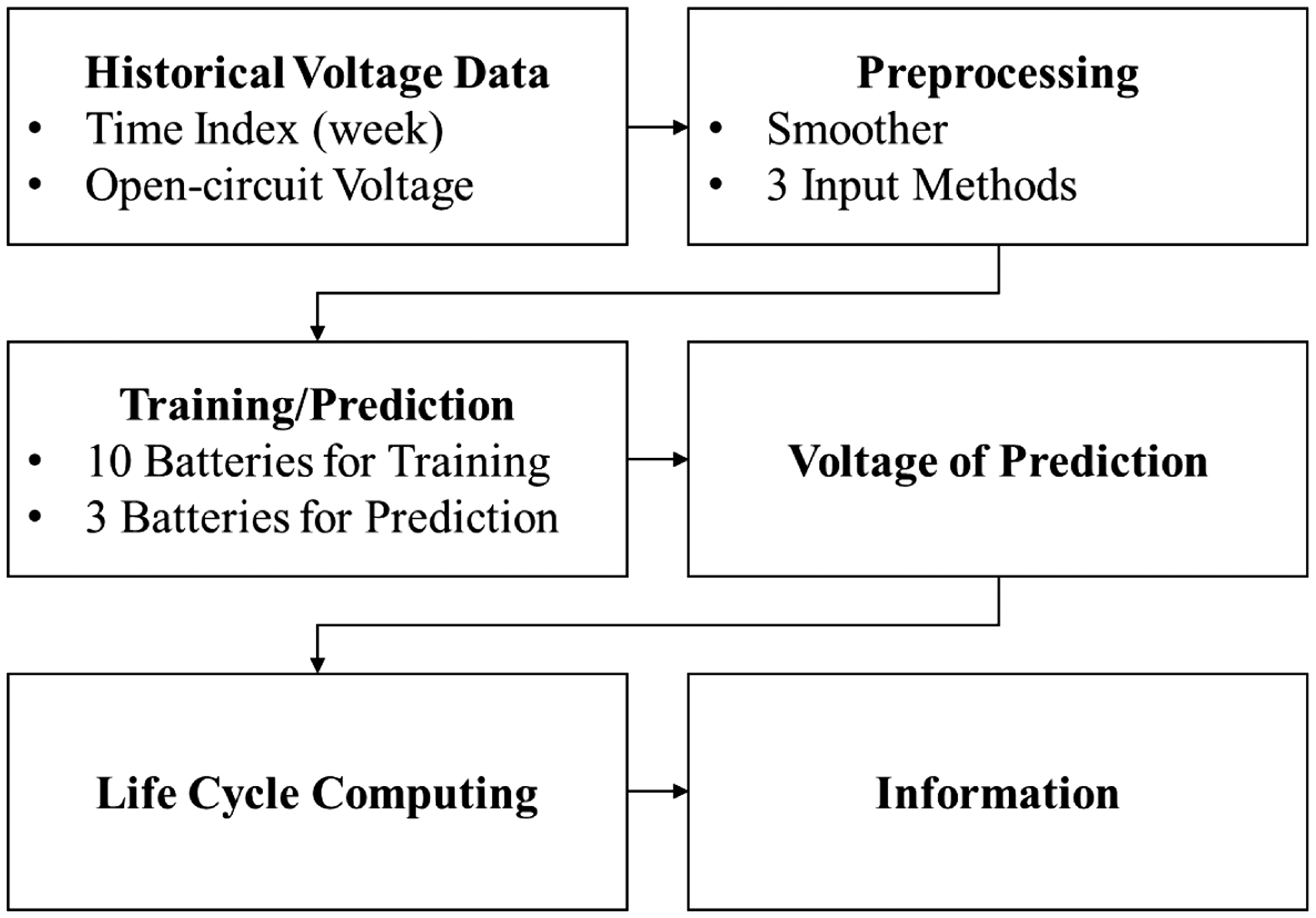
Block diagram of proposed architecture.

In the training phase, the historical voltage data of 10 batteries are used. In the test phase, three batteries are randomly selected for prediction. After obtaining the predicted voltage of the model output, the final battery life can be calculated according to the termination rule of the battery life. First collect the historical voltage data of the target battery, and find and establish the ideal life curve of the battery according to the model. All voltage data need to be normalized and standardized after obtaining the data. After completion, the original ideal life curve will be used as the default model. At this time, the prediction model is trained by CNN and MLP models, respectively. Upon completion of the training, complete analysis information and life prediction information can be obtained and the model can be considered based on the results of the training.

Dataset and preprocessing

The research goal is to use a lead–acid battery that is connected in series with six single cells, which is the power source for the electric vehicle. It will be used every day and battery is fully charged at night, and fixed at 8:00 am every Monday to measure the open circuit voltage of the battery after charging. In order to ensure experimental fairness, the operator of the vehicle does not know that the signals of these batteries will be recorded, thus maintaining routine operation. The data matrix in the experiment of this study came from 10 lead–acid batteries with the same model specifications, and randomly selected three (For the convenience of the name, the following three batteries are named by Batt A, Batt B, and Batt C.) for testing and prediction.

In signal processing, data smoothing preprocessing can be performed on the data through a smoothing filter. This process often captures important data and creates a new function that approximates the original function, while leaving noise or another fine structure/fast phenomenon. The original signal points are smoothed during the smoothing process, so each point (possibly due to noise) decreases and points below the adjacent point increase, resulting in a smoother signal. Smoothing can be used in two important ways to facilitate data analysis. The first is that smoothing assumptions can extract more information from the data if it is reasonable, and second, it can provide flexible and robust analysis (Egea-Roca et al., 2018; Xiao et al., 2018; Zhang et al., 2019).

Smoothing can be distinguished from the related and partially overlapping concepts of curve fitting in the following manner. Curve fitting usually involves using an explicit function form for the result, while the smooth direct result is a smooth value. The purpose of smoothing is to calculate the general concept of a relatively slow change in value, with little attention being paid to the close matching of the data values, while the curve fitting is concentrated as close as possible to the match. The smoothing method usually has associated adjustment parameters that are used to control the degree of smoothing. Curve fitting will adjust any number of parameters of the function to get the best fit.

Smoothing filters can be designed using many algorithms. This paper uses the moving average method as the core algorithm for data preprocessing. Moving averages are often used with time series data to eliminate short-term fluctuations and highlight long-term trends or cycle. The threshold between the short-term and long-term depends on the application, and the parameters of the moving average will be set accordingly.

Model of machine learning

There are many neural networks mentioned in “Introduction” section, including CNN, RNN, DNN, MLP, and SVM. Considering the characteristics of each neural network and the parameter type of the lead–acid battery, the CNN and MLP were chosen as models of neural networks in this research. More detail explanation are as follows.

MLP is a simple multi-input multi-output (MIMO) network with neural structure, which can be used in many classification applications. This method is an advanced method in the ANN and is also a feedforward conduction. The neural network mode includes an input layer, a hidden layer, and an output layer. The hidden layer of this mode may be one or more layers. It also allows non-linear function calculations, so it is very prominent in learning ability and is one of the most popular methods.

CNN is a relatively complex and large-scale MIMO neural network. The picture classification is the most common in classic applications. In the CNN network, the spatial structure features are well recognized because of the network in CNN. Attributes record the coordinate relationship between features, but with the maturity of neural network technology, CNN is not limited to the processing of images, and the variables input in this paper also have structural time characteristics, so CNN can be used to find features that change over time.

Therefore, in order to compare the effects of the two learning models using different features, the MLP and CNN models were designed for voltage prediction.

Model parameter design

Jupyter and Keras are used as tools for building learning models in this study. Table 1 shows the parameter to create the MLP architecture for learning model. The model expects rows of data with four variables. The MLP architecture is created with a sequential model. The first hidden layer has 32 nodes and uses relu activation function. The second hidden layer has 16 nodes and uses relu activation function. The output layer has one node and uses the normal activation function. Based on our need on prediction, regression loss is selected, which is mean square error. Adam optimizer is selected because it can automatically tune itself and gives good results in a wide range of problems.

Table 1.

MLP model construction parameter table.

No.	Design (MLP)
1	model = Sequential()
2	model.add(Dense(32, input_dim=4, init='normal', activation='relu'))
3	model.add(Dense(16, init='normal', activation='relu'))
4	model.add(Dense(1, init='normal'))
5	model.compile(loss="mse",optimizer='adam')

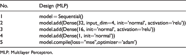
MLP: Multilayer Perceptron.

Table 2 shows the architectures of the proposed CNN model. The first hidden layer is a convolutional layer called a convolution2D. The convolution layer has four filters with a 2 × 2 kernel. A max pooling 2 D has a pool size of 2 × 2. The next layer is flatten, which has function to convert 2 D matrix data to 1 D vector. A fully connected layer with 32 neurons and relu activation are added in the network. A fully connected layer with 16 neurons and relu activation are added in the network. Finally, the output layer with one neuron is added into the network. The loss function and optimizer used the same function with MLP, which are mse and adam.

Table 2.

CNN model construction parameter table.

No.	Design (CNN)
1	model = Sequential()
2	model.add(Conv2D(4, kernel_size=(2, 2), input_shape=(2, 2, 3), activation='relu')
3	model.add(MaxPooling2D(pool_size=(2,2)))
4	model.add(Flatten())
5	model.add(Dense(32, activation='relu'))
6	model.add(Dense(16, activation='relu'))
7	model.add(Dense(1))
8	model.compile(loss="mse",optimizer='adam')

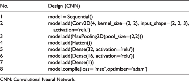
CNN: Convolutional Neural Network.

Model input and output variables

In order to achieve the best prediction effect of the trained model, this paper proposes three different ways to input test data to the same model to compare the predicted output prediction voltage. The three methods are shown in Table 3.

Table 3.

Three input data methods and expressions.

Call sign	Description and expression
M1	Use the four data from the starting point to predict future data, and re-predict the future from future data.
M1	$x_{[0]}, x_{[1]}, x_{[2]}, x_{[3]} \to y_{[i]}$
M2	Use the last four real data from the moment to predict the next data.
M2	${x_{[i - 4]}, x}_{[i - 3]}, x_{[i - 2]}, x_{[i - 1]} \to y_{[i]}$
M3	Use the last four real data from the moment to predict the next data. Recently, this data has a weighted relationship with the original prediction data, and then predicts the future.
M3	$x_{[i - 4]}, x_{[i - 3]}, x_{[i - 2]}, x_{[i - 1]} \times w_{1} + y_{[i - 1]} \times w_{2} \to y_{[i]}$

$x_{[i]}$ : the current value; $y_{[i]}$ : the future value being predicted; $w_{1}$ and $w_{2}$ are weights.

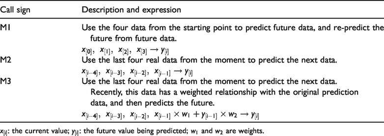
The first method, M1, uses only four data $x_{[0]}, x_{[1]}, x_{[2]}, x_{[3]}$ from the starting point to predict future data $y_{[i]}$ . The second method, M2, uses the most recent four real data ${x_{[i - 4]}, x}_{[i - 3]}, x_{[i - 2]}, x_{[i - 1]}$ to predict future data $y_{[i]}$ . The third method, M3, uses the recent four real data and the previous forecast data to perform weighting operations to predict future data. For example, after using $x_{[0]}, x_{[1]}, x_{[2]}, x_{[3]}$ to predict $y_{[4]}$ , predict $y_{[5]}$ with $x_{[1]}, x_{[2]}, x_{[3]}, (x_{[4]} \times w_{1} + y_{[4]} \times w_{2})$ .

Result

Preprocessing and modeling

In this paper, the MLP and CNN methods in ANN are used to predict the battery life. The training data set used in the training model is a time series related to decay voltage and time. Each column has 155 weeks of voltage data and a total of 10 columns. The system set the fail-off voltage is set to 11.5 V. The data preprocessing method is a smoothing algorithm using moving average, and smoothing is performed using the latest four consecutive data. Figure 2 shows the smoothed voltage data set. It can be seen from the waveform that the voltage enters the other linear attenuation region from the first linear attenuation region at about the 80th week.

Figure 2.

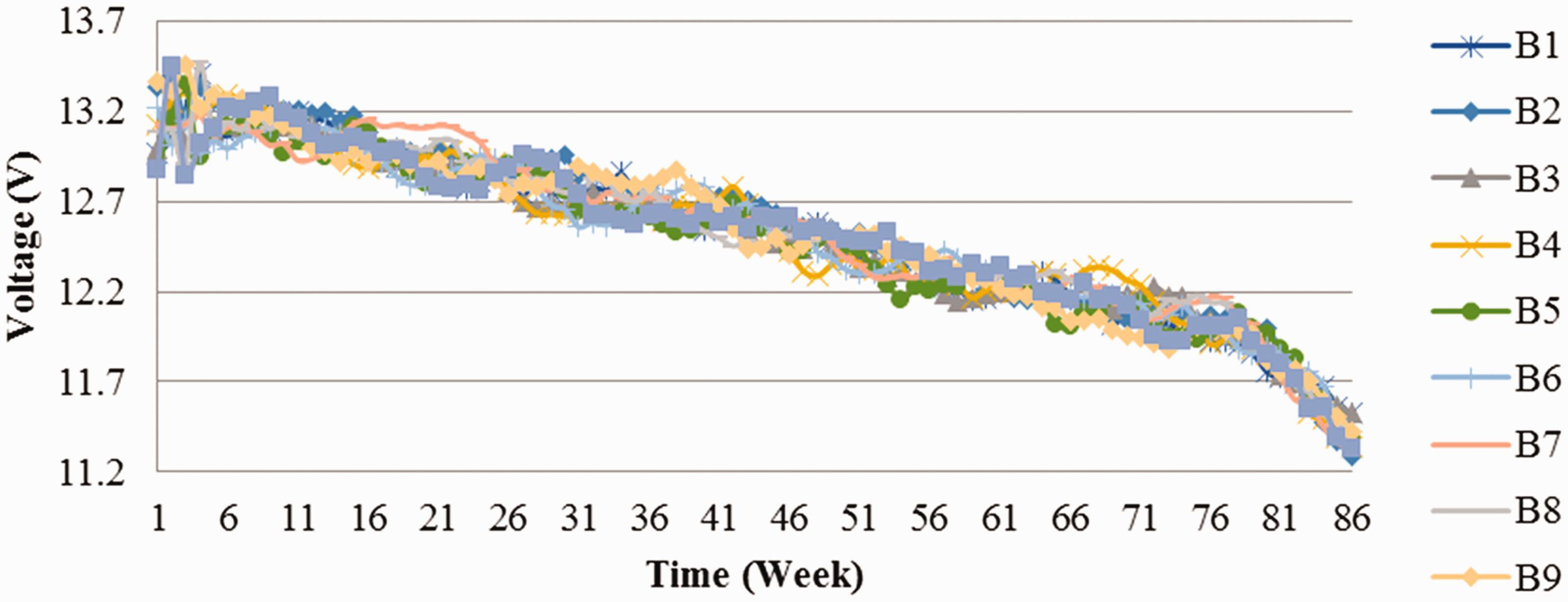
The smoothed raw voltage waveform, with a total of 10 battery data as a data set.

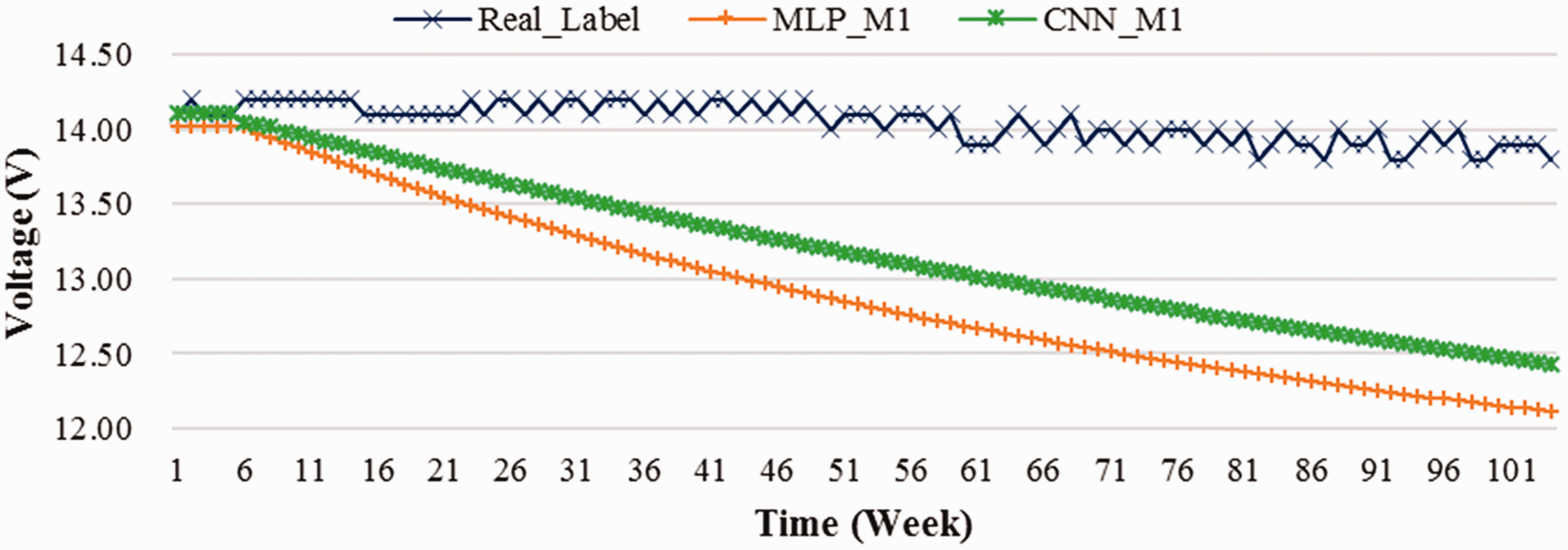
Method M1 used only the first to fourth data $x_{[0]}, x_{[1]}, x_{[2]}, x_{[3]}$ to predict future data $y_{[i]}$ . The next input data still uses $x_{[0]}, x_{[1]}, x_{[2]}, x_{[3]}$ for prediction of $y_{[i]}$ and so on. In other words, only fully linear data can be predicted. As shown in Figure 3, it is the prediction result obtained by the data input method M1. The prediction model obtained by M1 in the linear attenuation region before 70 weeks is the same as that of the real data, but after entering the second linear region, the prediction model still maintains the original trend until it cannot predict the change after 70 weeks.

Figure 3.

A comparison table of training results, using method M1 as an input to test the trained model of MLP and CNN.

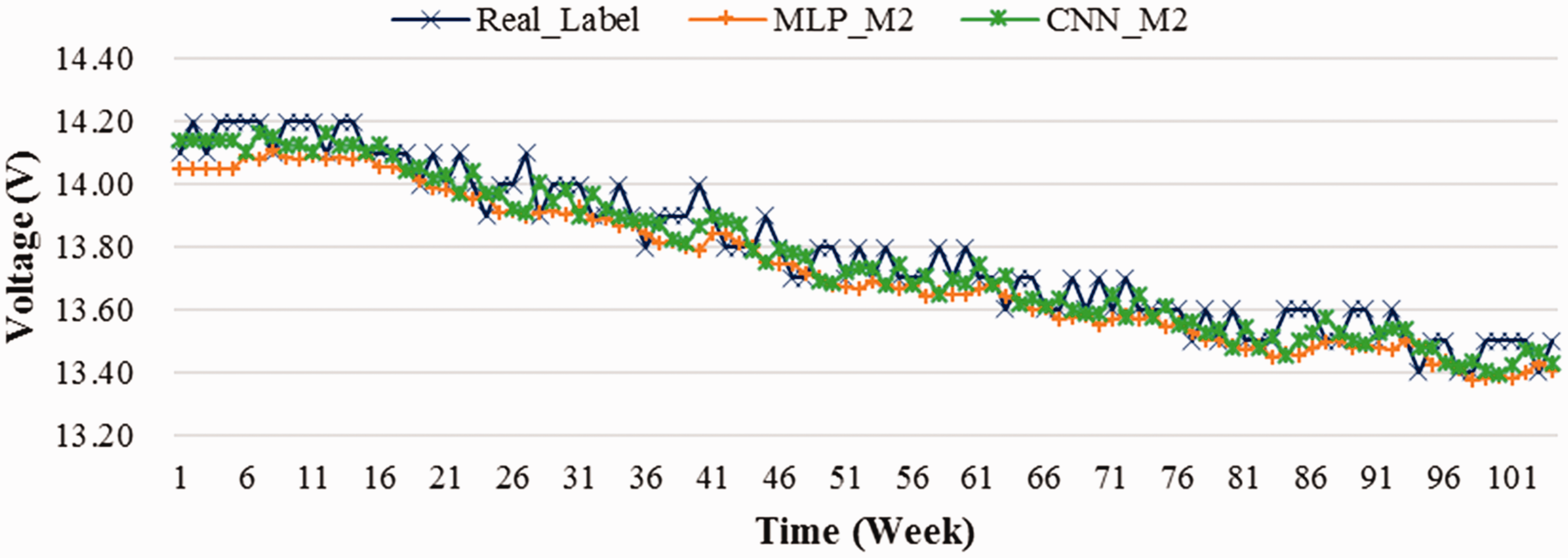
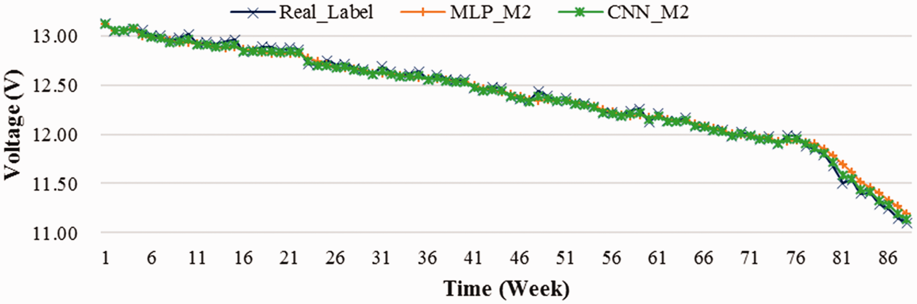
The second method M2 uses the recent four real data ${x_{[i - 4]}, x}_{[i - 3]}, x_{[i - 2]}, x_{[i - 1]}$ to predict the future data $y_{[i]}$ . Figure 4 shows the prediction result obtained by the data input method M2. The prediction model obtained by M2 in the linear attenuation zone before the 70th week is almost the same as the real data. After the line segment enters the second linear region, the prediction model can continue to conform to the changes of the original data. Compared to M1, the data are highly predictable at M2 after the 70th week.

Figure 4.

A comparison table of training results, using method M2 as an input to test the trained model of MLP and CNN.

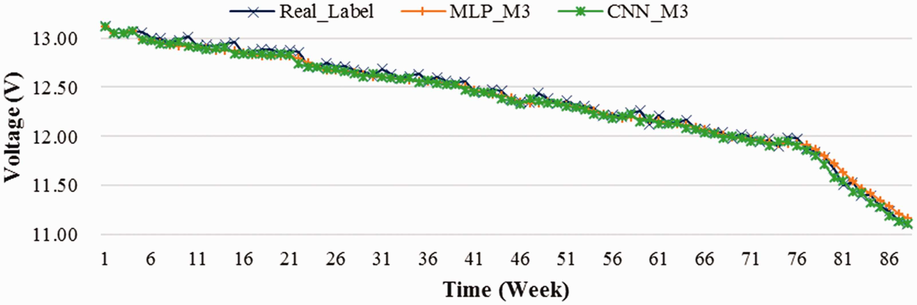
Method M3 uses the most recent four real data and the previous prediction data to perform a weighting operation $x_{[i - 4]}, x_{[i - 3]}, x_{[i - 2]}, (x_{[i - 1]} \times w_{1} + y_{[i - 1]} \times w_{2})$ to predict the future data $y_{[i]}$ . For example, after predicting $y_{[4]}$ in $x_{[0]}, x_{[1]}, x_{[2]}, x_{[3]}$ , $x_{[1]}, x_{[2]}, x_{[3]}, (x_{[4]} \times w_{1} + y_{[4]} \times w_{2})$ is used to predict $y_{[5]}$ . Figure 5 shows the prediction result obtained by the data input method M3. From the comparison between the MLP and CNN prediction models in the figure and the actual data, it can be known that the linear attenuation zone before the 70th week or the second linear zone after the 70th week can have a good prediction effect.

Figure 5.

A comparison table of training results, using method M3 as an input to test the trained model of MLP and CNN.

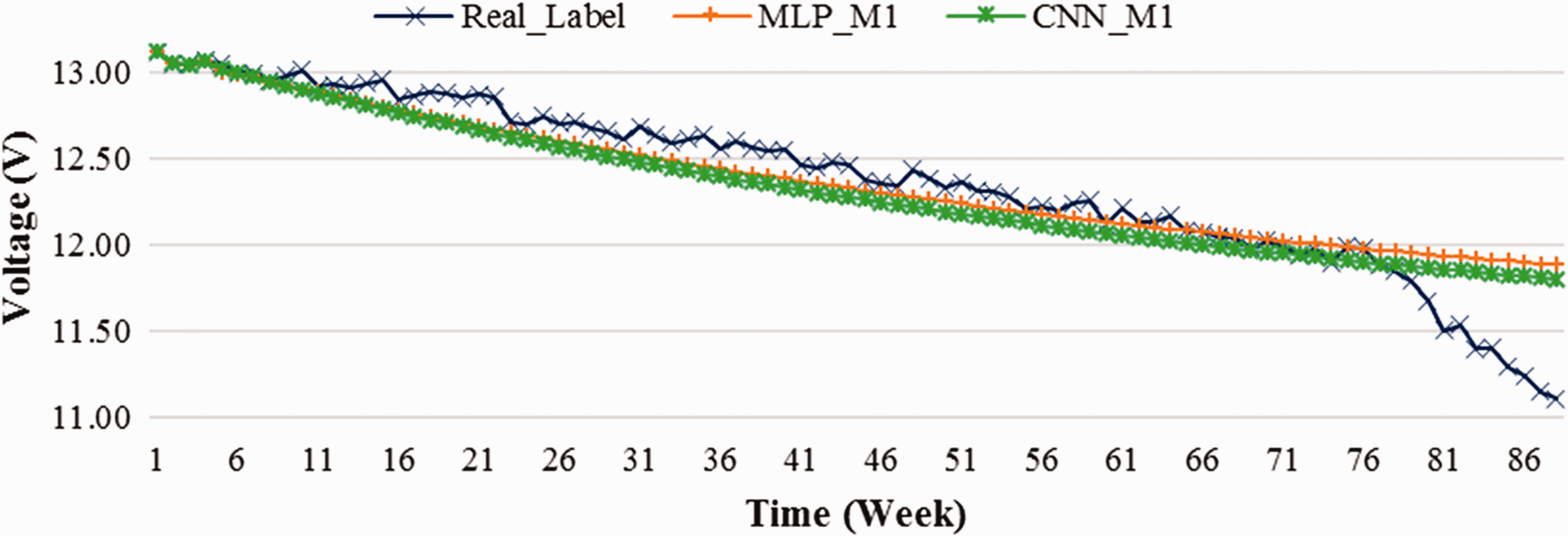
In this paper, the prediction models of MLP and CNN are used to predict the decay relationship between time and voltage. The system determines that it is necessary to update the battery if the open circuit voltage is lower than 11.5 V. Based on the calculation of current voltage and historical voltage data, the prediction model predicts the future voltage curve and predicts the number of life weeks that can be used in the future. Figure 6 shows a comparison of the predicted battery life between the MLP and CNN models. It can be seen that the predicted value and the actual value are only linear, but the curve itself will still fluctuate.

Figure 6.

Comparison of predicted result between MLP and CNN.

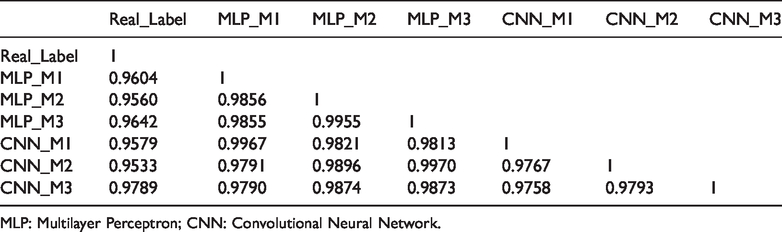
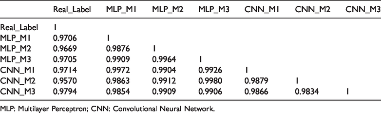
Three methods are used to input the same prediction model during the process of model training. The comparison in Table 4 is a method that uses the Pearson correlation coefficient to evaluate the correlation between predicted and actual values. The actual value (Real_Label) is used as a reference point to compare with the other six methods. It can be seen from the table that M1 has a correlation of only 0.93 with MLP and CNN. Although it is highly correlated in the pitch table defined in the Pearson correlation coefficient, M2 and M3 have up to 0.99 in MLP and CNN respectively; extremely highly correlated with MLP using M3 to get the best of all.

Table 4.

Correlation coefficient comparison table of output results using different input data methods (training phase).

	Real_Label	MLP_M1	MLP_M2	MLP_M3	CNN_M1	CNN_M2	CNN_M3
Real_Label	1
MLP_M1	0.9339	1
MLP_M2	0.9968	0.9472	1
MLP_M3	0.9975	0.9441	0.9996	1
CNN_M1	0.9329	1.0000	0.9462	0.9431	1
CNN_M2	0.9992	0.9406	0.9990	0.9995	0.9397	1
CNN_M3	0.9969	0.9364	0.9971	0.9984	0.9354	0.9980	1

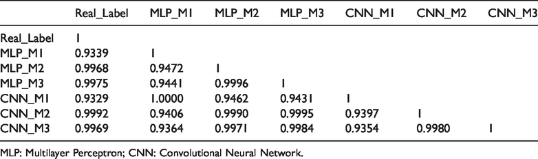
MLP: Multilayer Perceptron; CNN: Convolutional Neural Network.

Prediction result of Batt A

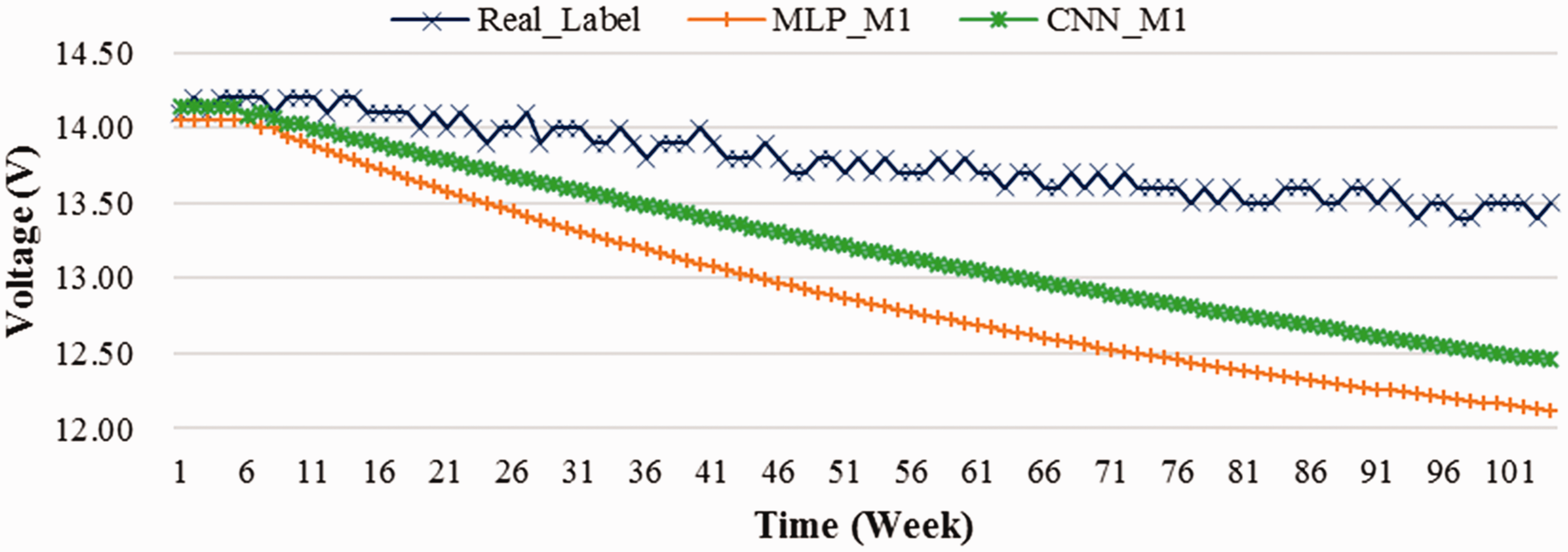
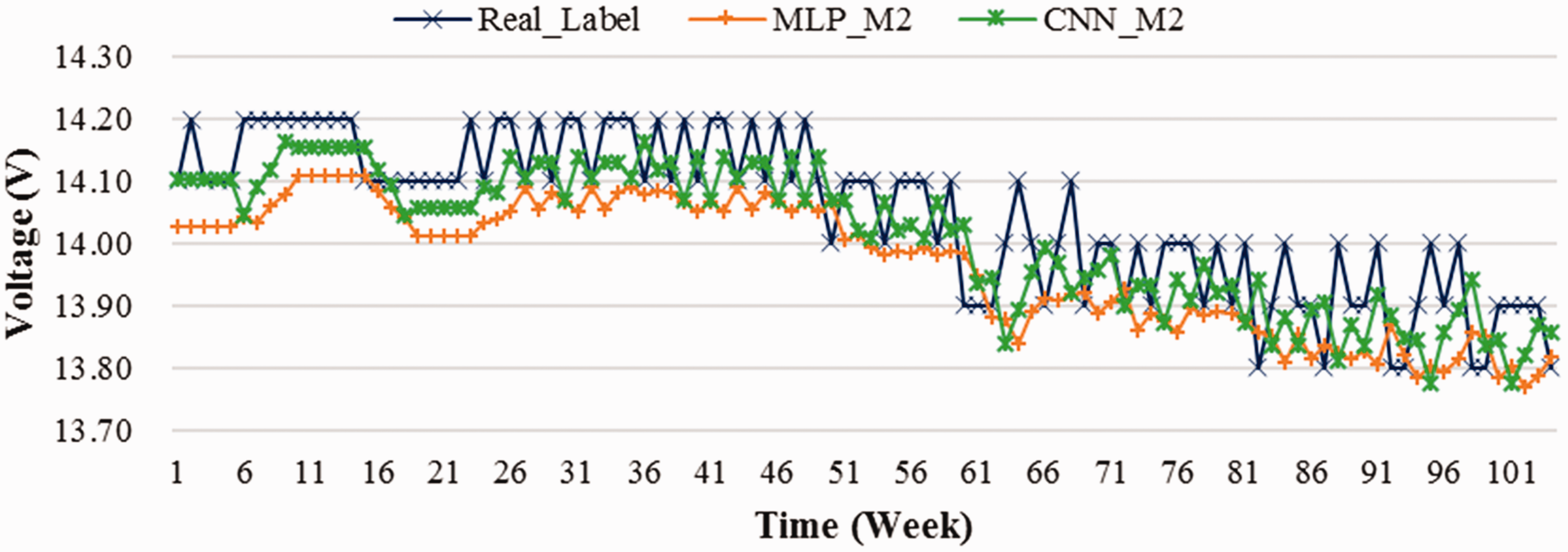
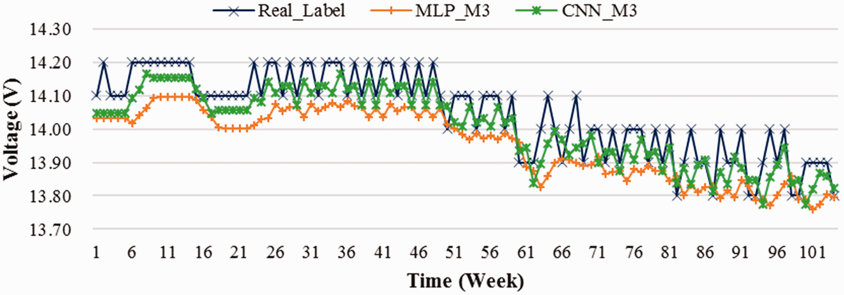
The model of the Batt A is predicted by the trained model as shown in Figures 7 to 9. Real_Label represents the actual data of Batt A, and the voltage prediction is performed using the input methods M1 to M3, respectively, for the trained model. Figure 7 shows that the original data tend to be linear and the negative slope decreases. The predicted results of MLP and CNN also decrease, but they are obviously separated from the original data. Figure 8 shows that the M2 method can be used to find that the prediction results are quite close to the original data. Figure 9 shows that the M3 method can find that the prediction results and trends are closer to the original data than M2.

Figure 7.

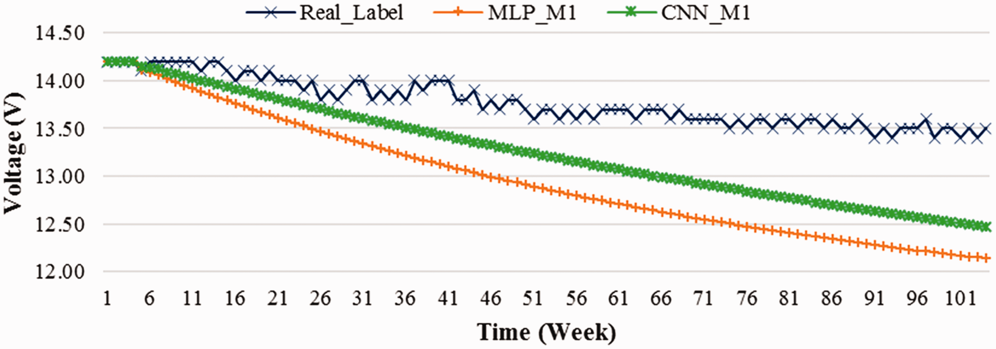
The prediction result comparison of Batt A in different model, using M1 as the input method to model.

Figure 8.

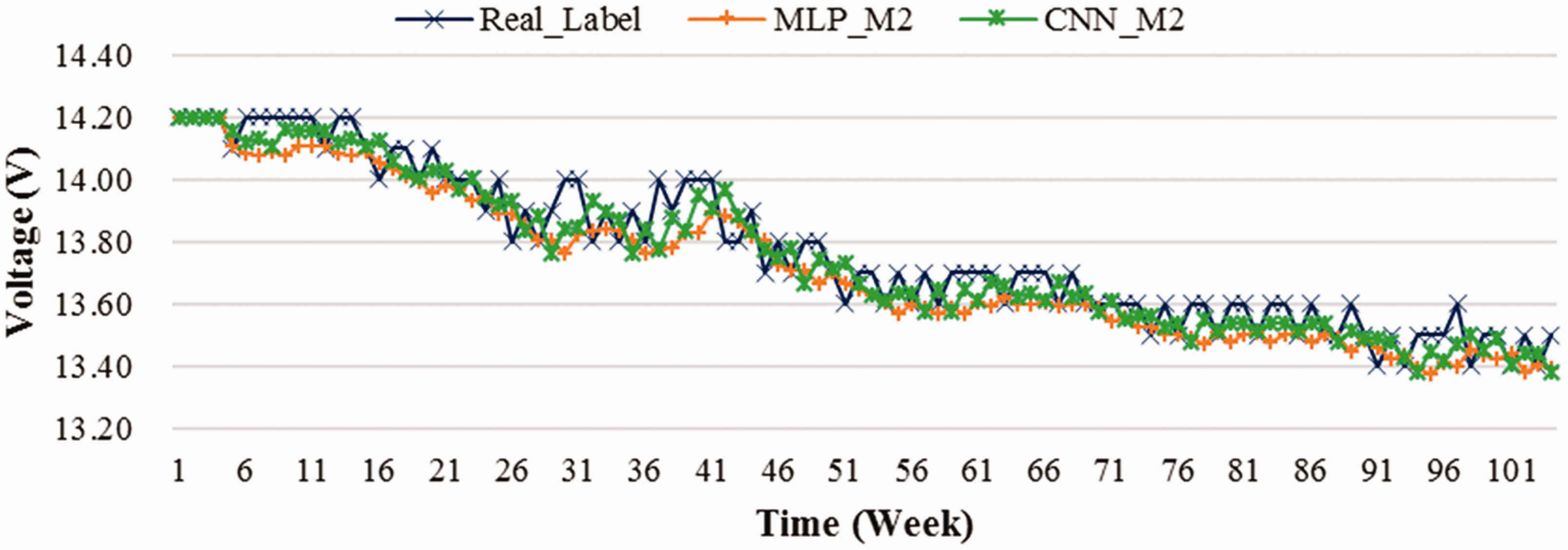
The prediction result comparison of Batt A in different model, using M2 as the input method to model.

Figure 9.

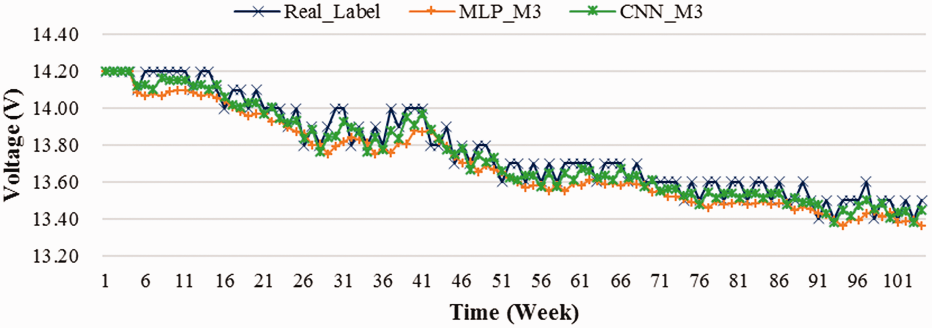
The prediction result comparison of Batt A in different model, using M3 as the input method to model.

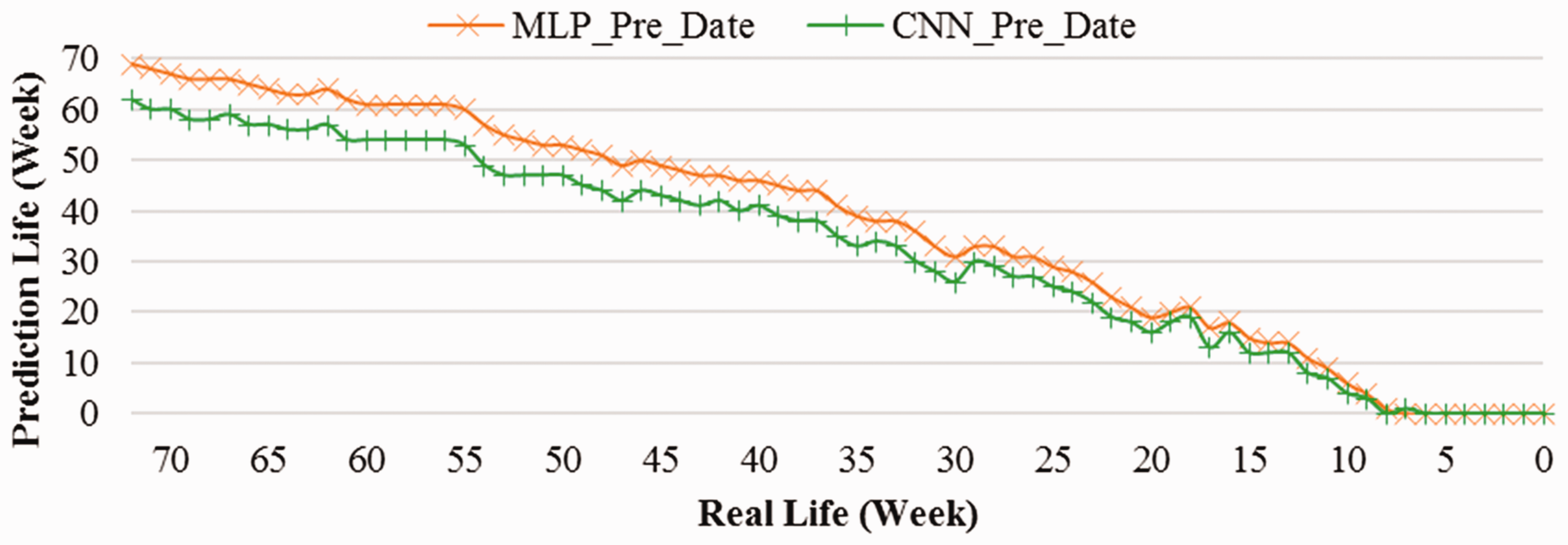
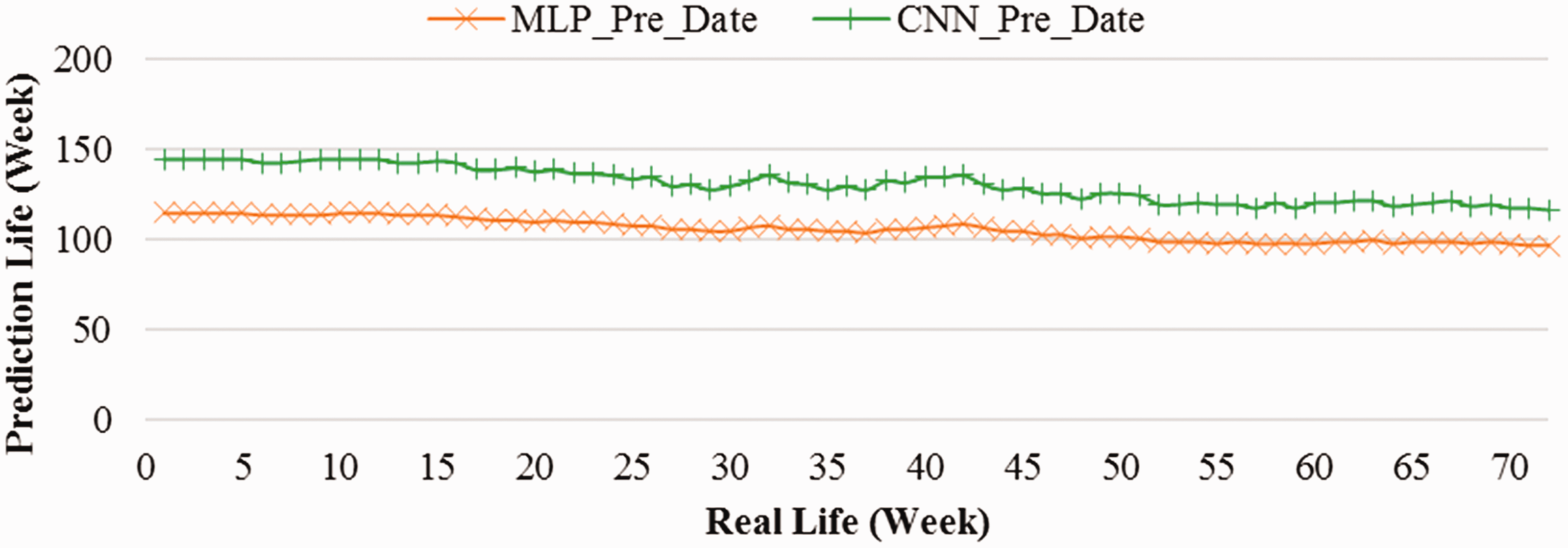
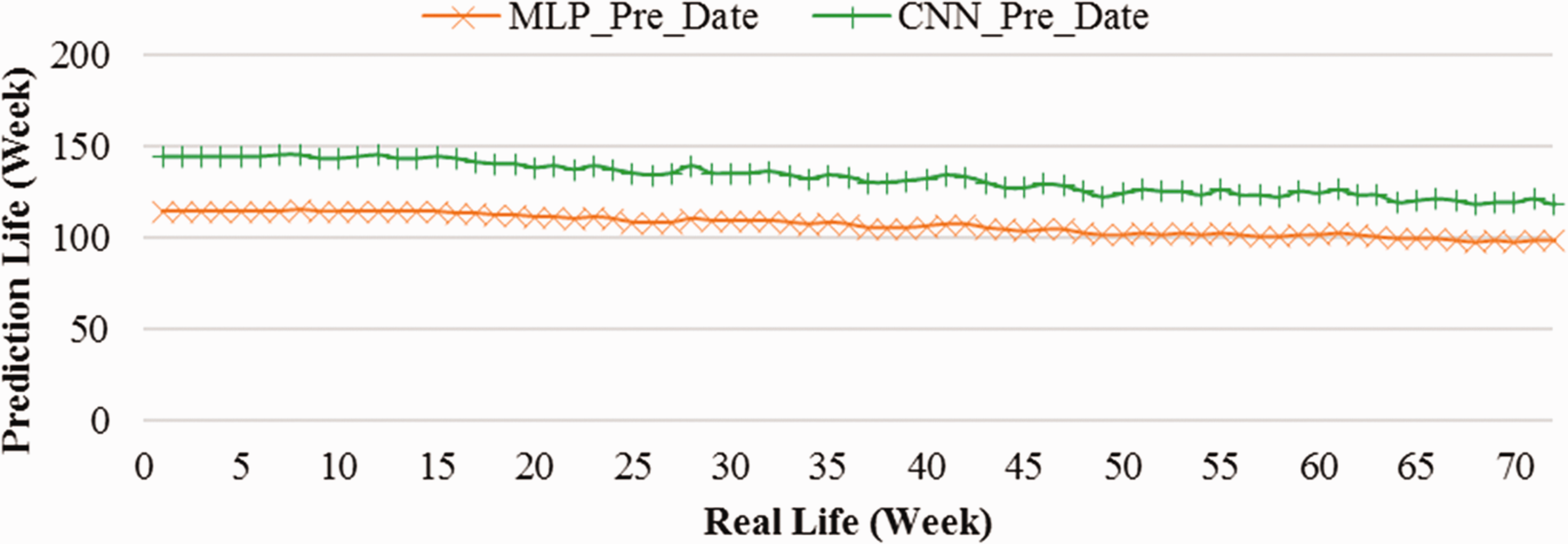
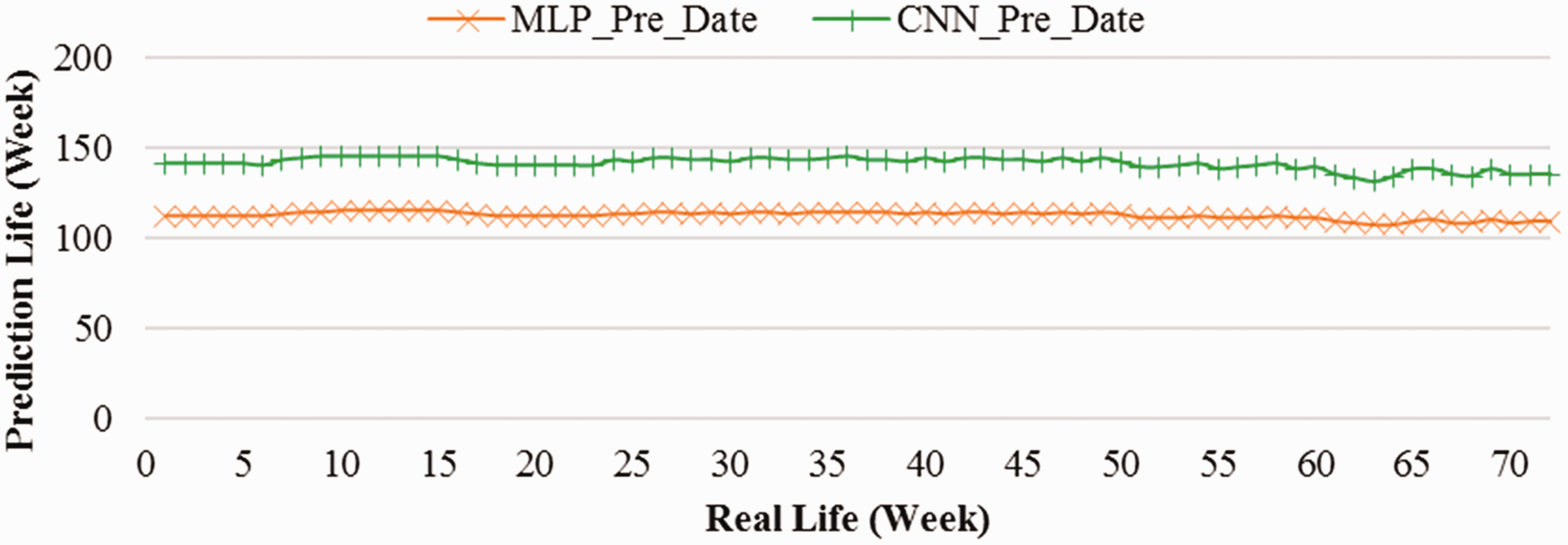
The life prediction chart of Batt A is shown in Figure 10. This figure shows the predicted life of the current Batt at any one point in time. Since the MLP and CNN models in this paper are based on the relationship between voltage and time, the effect of voltage on the prediction is very dramatic. It can be seen from the figure that the predicted time of the MLP model is lower than that predicted by CNN, because the model predicts the voltage influence in the predictions of Figures 7 to 9. In the above method, the predicted value of the MLP model is always smaller than the value predicted by the CNN model, and finally the time for MLP prediction is shorter than that of CNN.

Figure 10.

Comparison of life prediction results of Batt A under different networks.

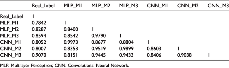
Table 5 shows the correlation of actual values with the other six methods. It can be seen from the table that the correlation between each method and the original data falls within the range of 0.956–0.978, which is highly correlated within the pitch table defined in the Pearson correlation coefficient. M3 in MLP and CNN are the best results in this model.

Table 5.

Comparison table of correlation coefficients of Batt A in prediction results.

	Real_Label	MLP_M1	MLP_M2	MLP_M3	CNN_M1	CNN_M2	CNN_M3
Real_Label	1
MLP_M1	0.9604	1
MLP_M2	0.9560	0.9856	1
MLP_M3	0.9642	0.9855	0.9955	1
CNN_M1	0.9579	0.9967	0.9821	0.9813	1
CNN_M2	0.9533	0.9791	0.9896	0.9970	0.9767	1
CNN_M3	0.9789	0.9790	0.9874	0.9873	0.9758	0.9793	1

MLP: Multilayer Perceptron; CNN: Convolutional Neural Network.

Prediction result of Batt B

The original curve of Batt B and Batt A is very similar. It can be seen from Figure 11 that the predicted voltage of MLP is still lower than the voltage predicted by CNN when inputting data by M1 method. Figure 12 shows that the M2 method can be used to find that the predicted voltages of MLP and CNN are very close to the original data, but the prediction point is still oscillating near the original data. Figure 13 shows that the M3 method is used to predict better results than M2. Compared with M1 and M2, M3 makes the data closer and reduces more oscillations, which improves the prediction accuracy.

Figure 11.

The prediction result comparison of Batt B in different model, using M1 as the input method to model.

Figure 12.

The prediction result comparison of Batt B in different model, using M2 as the input method to model.

Figure 13.

The prediction result comparison of Batt B in different model, using M3 as the input method to model.

The life prediction chart of Batt B is shown in Figure 14. Since the voltage raw signal of the Batt B is more stable than the Batt A, the life prediction is also stable and decreases with time. From the original data, we can find that the initial voltages of Batt A and Batt B are very similar, so the results of life prediction are similar. However, due to the prediction model training, the predicted number of days of MLP is still lower than that predicted by CNN.

Figure 14.

Comparison of life prediction results of Batt B under different networks.

Table 6 shows the correlation between the actual values and the other six methods. It can be seen from the table that the correlation between each method and the original data falls within the range of 0.957–0.979, where M1 is the best result in MLP and M3 in CNN. Although the result of comparison from the drawing is that the input modes M2 and M3 are closer to the original data than M1. However, the Pearson correlation coefficient is calculated in such a way that M1 looks better than M2.

Table 6.

Comparison table of correlation coefficients of Batt B in prediction results.

	Real_Label	MLP_M1	MLP_M2	MLP_M3	CNN_M1	CNN_M2	CNN_M3
Real_Label	1
MLP_M1	0.9706	1
MLP_M2	0.9669	0.9876	1
MLP_M3	0.9705	0.9909	0.9964	1
CNN_M1	0.9714	0.9972	0.9904	0.9926	1
CNN_M2	0.9570	0.9863	0.9912	0.9980	0.9879	1
CNN_M3	0.9794	0.9854	0.9909	0.9906	0.9866	0.9834	1

MLP: Multilayer Perceptron; CNN: Convolutional Neural Network.

Prediction result of Batt C

The predicted results of Batt C are shown in Figures 15 to 17. Figure 15 shows that the prediction curves of MLP and CNN are not close to the real data, and it can be found from the figure that the true voltage curve of Batt C is different from the former two. Instead, it suddenly drops at the 51st week and falls again at 81 weeks. The curve is similar to the step function. Figure 16 shows that after using the M2 method, it can be found that the predicted data are close to the target data and then fluctuates. Due to the instability of the original voltage data, the prediction results show that the MLP is not always lower than CNN. Figure 17 shows the prediction results using the M3 method. It can be seen from the graph that although the M2 and M3 methods all obtain fairly similar prediction results, the M2 prediction results are not as accurate as the M3 prediction results.

Figure 15.

The prediction result comparison of Batt C in different model, using M1 as the input method to model.

Figure 16.

The prediction result comparison of Batt C in different model, using M2 as the input method to model.

Figure 17.

The prediction result comparison of Batt C in different model, using M3 as the input method to model.

Figure 18 shows the life prediction chart of the Batt C. The voltage signal of Batt C is unstable and decreases, but the magnitude of the decrease is small, so the predicted attenuation amplitude in life is relatively flat. However, due to the prediction model training, the prediction results of CNN are still higher than those predicted by MLP.

Figure 18.

Comparison of life prediction results of Batt C under different networks.

Table 7 shows the correlation between the actual value and the other six methods. It can be seen from the table that the correlation between each method and the original data falls within the range of 0.784–0.907. Among them, M3 is the best result in MLP and CNN. Due to the sudden change in voltage during the 51st and the 81st weeks, the nonlinear change caused the model to use the M1 and M2 methods to reduce the prediction accuracy. The M3 uses the past and future data to increase the accuracy.

Table 7.

Comparison table of correlation coefficients of Batt C in prediction results.

	Real_Label	MLP_M1	MLP_M2	MLP_M3	CNN_M1	CNN_M2	CNN_M3
Real_Label	1
MLP_M1	0.7842	1
MLP_M2	0.8287	0.8400	1
MLP_M3	0.8594	0.8542	0.9790	1
CNN_M1	0.8052	0.9973	0.8677	0.8804	1
CNN_M2	0.8007	0.8353	0.9519	0.9899	0.8603	1
CNN_M3	0.9070	0.8151	0.9445	0.9433	0.8406	0.9038	1

MLP: Multilayer Perceptron; CNN: Convolutional Neural Network.

Discussion

This paper uses MLP and CNN to establish a battery voltage decay model to predict battery life. The voltage prediction of the three batteries is performed using three different data input formats. The first method M1 uses the first four data for prediction. The second method, M2, uses the latest four data in the past to make predictions. The third method, M3, uses the latest four data in the past and the previous predicted data for future prediction.

The MLP and CNN models were trained using 10 training sets and tested with one test set. The convergence was completed five times during the training process, and the oscillations were found at the 6th to 10th training. After the training is completed, M1, M2 and M3 are, respectively, used to input MLP and CNN for testing. M1 has a correlation of 0.93 in MLP and CNN, and M2 and M3 have a very high correlation with MLP and CNN up to 0.99, respectively. Compared with the original data, which has a linear trend and a linear change, the prediction model of M1 is almost a linear equation, and the prediction results of M2 and M3 are close to the original voltage data, so the correlation of M1 is slightly lower than M2 and M3.

The raw voltage data of Batt A and Batt B is a segment that exhibits linear trend attenuation and no sudden attenuation, so the M1 and M2 mode input MLP and CNN are highly correlated. However, since the trend of M1 is the same as the trend of the original data, M2 is partially misaligned due to the training process, so that the accuracy of M2 is actually higher than M1 but the correlation result is reversed. Batt C, which decays twice in the 51st and 81st weeks, causes linear prediction misalignment of M1, and M2 can maintain a high correlation because it uses the most recent data for prediction.

Since the M1 data input method is used on a non-linearly attenuated battery, it will face a large misalignment problem. While M2 can use the latest four actual data to make predictions, it can get good accuracy; but the prediction results cannot fully predict the trend. Therefore, M3 uses the latest four data in the past and the previous forecast data for future forecasting, and obtains the highest correlation among the various methods.

Conclusion

ANNs can solve many complex problems that could not be solved in the past. There are many kinds of neural models in the neural network to solve different types of problems. Since lead–acid batteries are still the main source of electricity in many vehicles, their life prediction is a very important issue. This paper uses MLP and CNN to establish a voltage decay model of lead–acid battery to predict battery life. First, 10 prediction models are built through 10 data training sets and tested using one test set. Three different data input methods are compared to predict the model. As a result, the life prediction of three batteries was finally randomized.

Compared with the training model of CNN in three batteries, CNN obtained higher accuracy than MLP. The results show that using the M1 data on a non-linearly attenuated battery presents a significant misalignment problem. Using M2 can predict a more accurate attenuation voltage, but it is not suitable for use in widely changing applications. Using M3, the attenuation voltage can be predicted most accurately, and it is also the best data input method in each mode.

According to our research on lead–acid battery voltage prediction, we give the following conclusions and suggestions: (1) the selected prediction model has more input parameters such as CNN; (2) the input parameters need to have a timing relationship; and (3) complex network models can extract tiny features.

Footnotes

Declaration of conflicting interests

The author(s) declared no potential conflicts of interest with respect to the research, authorship, and/or publication of this article.

Funding

The author(s) disclosed receipt of the following financial support for the research, authorship, and/or publication of this article: This work was supported by the “Allied Advanced Intelligent Biomedical Research Center, STUST” under Higher Education Sprout Project, Ministry of Education, Taiwan.

References

Alanis

(2018) Electricity prices forecasting using artificial neural networks. IEEE Latin America Transactions 16(1): 105–111.

Ali

Zafar

Nengroo

et al. (2019) Towards a smarter battery management system for electric vehicle applications: A critical review of lithium-ion battery state of charge estimation. Energies 12(3): 446.

Álvarez Antón

García Nieto

de Cos Juez

, et al. (2013) Battery state-of-charge estimator using the SVM technique. Applied Mathematical Modelling 37(9): 6244–6253.

Berecibar

(2019) Machine-learning techniques used to accurately predict battery life. In Nature 568: 325–326.

Chaoui

Ibe-Ekeocha

Gualous

(2017) Aging prediction and state of charge estimation of a LiFePO4 battery using input time-delayed neural networks. Electric Power Systems Research 146: 189–197.

Chien

Chen

(2018) A multilayer perceptron-based impulsive noise detector with application to power-line-based sensor networks. IEEE Access 6: 21778–21787.

Egea-Roca

López-Salcedo

Seco-Granados

, et al. (2018) Performance bounds for finite moving average tests in transient change detection. IEEE Transactions on Signal Processing 66(6): 1594–1606.

Elliott

(1999) Abraham Bennet F.R.S. (1749–1799): A provincial electrician in eighteenth-century England (PDF). Notes and Records of the Royal Society of London 53(1): 59–78.

Hinchi

Tkiouat

(2018) A deep long-short-term-memory neural network for lithium-ion battery prognostics. In: Proceedings of the international conference on industrial engineering and operations management, Paris, France, 26–27 July, pp.2162–2168.

10.

Homan

ten Kortenaar

Hurink

, et al. (2019) A realistic model for battery state of charge prediction in energy management simulation tools. Energy 171: 205–217.

11.

Isogawa

Ida

Shiodera

, et al. (2018) Deep shrinkage convolutional neural network for adaptive noise reduction. IEEE Signal Processing Letters 25(2): 224–228.

12.

Khumprom

Yodo

(2019) A data-driven predictive prognostic model for lithium-ion batteries based on a deep learning algorithm. Energies 12(4): 660.

13.

Kurzweil

(July 2010) Gaston Planté and his invention of the lead–acid battery—The genesis of the first practical rechargeable battery. Journal of Power Sources 195(14): 4424–4434.

14.

Laayouj

Jamouli

(2015) Remaining useful life prediction of lithium-ion battery degradation for a hybrid electric vehicle. Global Advanced Research Journal of Engineering 4(2): 16–23.

15.

Wang

Chao

K-H

, et al. (2016) Remaining useful life prediction for lithium ion batteries based on Gaussian processes mixture. Plos One 11(9): e0163004.

16.

Liang

Hong

Xie

, et al. (2018) Combining convolutional neural network with recursive neural network for blood cell image classification. IEEE Access 6: 36188–36197.

17.

Lin

Tseng

Wen

, et al. (2018) Reconstruction algorithm for lost frame of multiview videos in wireless multimedia sensor network based on deep learning multilayer perceptron regression. IEEE Sensors Journal 18(23): 9792–9801.

18.

Liu

Saxena

Goebel

, et al. (2010) An adaptive recurrent neural network for remaining useful life prediction of lithium-ion batteries. In: Annual conference of the prognostics and health management society, Portland, OR, 10-16 October, pp.1–9.

19.

Liu

Peng

, et al. (March 2019) A brief review on key technologies in the battery management system of electric vehicles. Frontiers of Mechanical Engineering 14(1): 47–64.

20.

Lyu

Lai

, et al. (2017) A lead-acid battery’s remaining useful life prediction by using electrochemical model in the Particle Filtering framework. Energy 120: 975–984.

21.

Marcel

Sander

(2017) Editorial: Artificial neural networks as models of neural information. In Frontiers in Computational Neuroscience 11: 114.

22.

McCulloch

Pitts

(December 1943) A logical calculus of the ideas immanent in nervous activity. The Bulletin of Mathematical Biophysics 5(4): 115–133.

23.

Ren

Zhao

Hong

, et al. (2018) Remaining useful life prediction for lithium-ion battery: A deep learning approach. IEEE Access 6: 50587–50598.

24.

Rezvani

AbuAli

Lee

, et al. (2011) A comparative analysis of techniques for electric vehicle battery prognostics and health management (PHM). SAE Technical Paper 2011-01-2247. Epub ahead of print 13 September 2011. DOI: 10.4271/2011-01-2247.

25.

Salameh

El Ghossein

El Hassan

, et al. (April 2017) Battery modeling and lifetime prediction. Modern Environmental Science and Engineering 3(4): 278–290.

26.

Song

Yang

Wang

, et al. (2019) Combined CNN-LSTM network for state-of-charge estimation of lithium-ion batteries. IEEE Access 7: 88894–88902.

27.

Voronov

Frisk

Krysander

(June 2018) Data-driven battery lifetime prediction and confidence estimation for heavy-duty trucks. IEEE Transactions on Reliability 67(2): 623–639.

28.

Whittingham

(June 1976) Electrical energy storage and intercalation chemistry. Science 192(4244): 1126–1127.

29.

Wibawa

Pratama

Nur Hasanah

(2017) Lifetime prediction of lead-acid batteries in base-transceiver station. International Journal on Advanced Science, Engineering and Information Technology 7(4): 1361–1366.

30.

Xiang

Tran

Johnson

(2018) Output reachable set estimation and verification for multilayer neural networks. IEEE Transactions on Neural Networks and Learning Systems 29(11): 5777–5783.

31.

Xiao

Butlin

Qasem

, et al. (June 2018) N-point moving average: A special generalized transfer function method for estimation of central aortic blood pressure. IEEE Transactions on Biomedical Engineering 65(6): 1226–1234.

32.

Zhang

Liang

Zhang

(2017) An overview of different approaches for battery lifetime prediction. Iop Conference Series: Materials Science and Engineering 199(1): 1–6.

33.

Zhang

Wang

Zhang

, et al. (2019) Learning spatial–spectral–temporal EEG features with recurrent 3D convolutional neural networks for cross-task mental workload assessment. IEEE Transactions on Neural Systems and Rehabilitation Engineering 27(1): 31–42.

34.

Zhang

Xiong

, et al. (July 2018) Long short-term memory recurrent neural network for remaining useful life prediction of lithium-ion batteries. IEEE Transactions on Vehicular Technology 67(7): 5695–5705.

35.

Zhang

Qiao

Zhang

, et al. (2019) Fractional weight moving average based thresholding scheme for VLC with mobile-phone camera. IEEE Photonics Journal 11(1): 1–8.

A prediction method for voltage and lifetime of lead–acid battery by using machine learning

Abstract

Keywords

Introduction

Method

Proposed method description

Dataset and preprocessing

Model of machine learning

Model parameter design

Model input and output variables

Result

Preprocessing and modeling

Prediction result of Batt A

Prediction result of Batt B

Prediction result of Batt C

Discussion

Conclusion

Footnotes

Declaration of conflicting interests

Funding

References