Sage Journals: Discover world-class research

Abstract

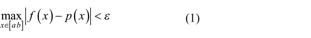
This article deals with fabric defect detection. The quality control in textile manufacturing industry becomes an important task, and the investment in this field is more than economical when reduction in labor cost and associated benefits are considered. This work is developed in collaboration with “PARTNER TEXTILE” company which expressed its need to install automated defect fabric detection system around its circular knitting machines. In this article, we present a new fabric defect detection method based on a polynomial interpolation of the fabric texture. The different image areas with and without defects are approximated by appropriate interpolating polynomials. Then, the coefficients of these polynomials are used to train a neural network to detect and locate regions of defects. The efficiency of the method is shown through simulations on different kinds of fabric defects provided by the company and the evaluation of the classification accuracy. Comparison results show that the proposed method outperforms several existing ones in terms of rapidity, localization, and precision.

Keywords

Fabric defect detection polynomial interpolation multilayer perceptron

Introduction

As the global market puts higher and higher demand on product quality, automated inspection has increasingly developed in recent years in all areas such as manufacture of mechanical parts and electronic boards.^1–6

Defect detection is one of the main steps in quality control in industry. Various defect detection systems are now installed in different production lines such as defect detection of tiles,⁷ woods,^8,9 ceramic,¹⁰ and sheet steel.¹¹

In fabric manufacturing, about 85% of the defects found in the garment industry are caused by fabric defects. Consequently, it becomes imperative to detect and prevent any defect from appearing.

A fabric defect can be considered as a variation of the neighborhood property caused by a wired variation with respect to the overall surface aspect. In our country Tunisia, a large part of the national economy is based on textiles. Until now, some industries have not yet installed automated defect detection systems and they use simple human inspection. This leads to multiple errors due to many reasons, namely, the fatigue and fine defects. Automated fabric inspection is at least four times faster than visual inspection.⁶ Hence, the automation of these operations helps to improve quality and to reduce labor costs.

In this framework, this work is developed in collaboration with “PARTNER TEXTILE” company from Tunisia.¹² This is later specialized in the manufacture of different fabric types. Due to the huge production capacity (about 6 tons/day), the company aims at equipping its machines by efficient defect detection systems that can be easily installed around circular knitting machines (Figure 1).

Figure 1.

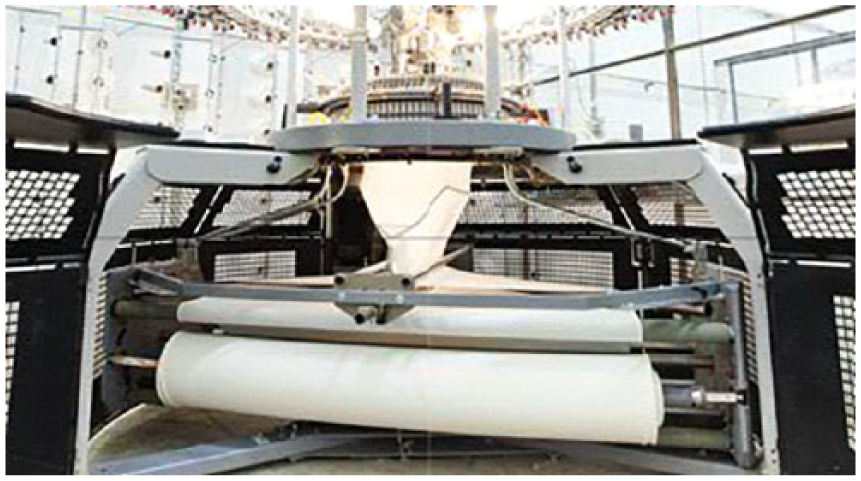
Circular knitting machines.

In literature, one can find variety of image processing methods and propositions for automated defect detection. Some of these methods cannot be easily used or installed in the production lines for several reasons, namely, the complexity, the limitation on a very special type of images, the non-robustness to noise and to reasonable variations of the image or the object shapes, and the imprecision.

To develop defect detection methods, several methods based on signal and image processing tools have been used in literature such as co-occurrence matrices, correlation and covariance matrices, Fourier and wavelet transform, and distance and gradient approximation.

In Latif-Amet et al.,¹³ authors proposed a combination strategy between wavelet transform and co-occurrence matrices to develop a defect detection algorithm for textile images. Gabor filters (GFs) have been likewise widely used in the field of fabric defect detection. Methods based on GFs can be classified into two types. The first consists in the use of a filter bank, such as in Kumar and Pang.¹⁴ The second consists in the search for the optimal filters, such as in Hamid et al.¹⁵ and Bodnarova et al.¹⁶ Note that the use of a filter bank generates in general excessive data, which becomes sometimes hard to deal with.

Viewed as exceptional and robust classification tools, neural networks have been widely used in the field of defect detection. Indeed, by choosing appropriate features, an artificial neural network can be applied to classify and separate defects from defect-free regions. Due to their generalization capacities, neural networks can efficiently surpass the problem of feature variations in the same defect-free regions as well as in regions with defects. For example, Kumar¹⁷ used a multilayer neural network to classify principal components of regions with defect and with no defects. Principal components are extracted directly from each pixel within its neighborhood. In Huang and Chen,¹⁸ a neural network with fuzzy logic strategy was used to propose a classification algorithm of eight different fabric defects.

In this work, we develop a new defect detection method based on polynomial interpolation of a set of a pixel and its neighborhood to extract feature database to be used to train a multilayer perceptron (MLP). The presented method highlights several other existing methods in terms of rapidity, localization, and precision.

The efficiency of the method is shown through simulations, the evaluation of the classification accuracy (CA), and comparisons. For simulations, we used a set of 76 images provided by the company. In these images, defect areas are well known and localized by the experts of the company.

This article is organized as follows: in section “New defect detection scheme,” a description of the new defect detection scheme is provided, while in section “Newton form of the interpolating polynomial and its application to the V₂₄ Neighborhood,” the Newton form of the interpolating polynomial is given followed by its application to the V₂₄ Neighborhood. The MLP and the modified backpropagation algorithm are then described in section “MLP description.” Section “Simulations” is devoted to the description of the database presentation and the different simulation results. A performance evaluation and comparison results are furthermore detailed in this section. Finally, this article provides general conclusions and perspectives.

New defect detection scheme

The key issue in the texture defect detection field is to determine the way by which one can characterize the texture (i.e. the use of appropriate models or discriminant features). Then, the defect detection involves searching the variations in the model or its features.

Due to the wide variety of textures, an exhaustive determination of all feature sets to characterize these textures is a tedious task. In order to overcome these difficulties, we propose to characterize the texture by a set of interpolation polynomials for each pixel with respect to its neighboring pixels defined by a pre-chosen mask. In image processing, the choice of the appropriate mask is an important task and plays a significant role in the final results. In this work, we propose to use a V₂₄ neighborhood mask in a 7 × 7 macro window as given in Figure 2.¹⁹ The main property of such mask lies in the fact that it allows to study each pixel in a large neighborhood for different directions. This permits to well perceive the variation with respect to the overall surface aspect.

Figure 2.

Definition of the neighborhood of a central pixel in a 7 × 7 macro window forming a V₂₄ mask.

This V₂₄ mask presents four directions $0, π / 4, π / 2$ , and $3 π / 4$ with respect to the central pixel. As shown in Figure 3, each seven points in one direction can be joined by a polynomial curve obtained by an interpolation algorithm. The interpolation polynomial for each direction will be then of degree less or equal to 6 having 7 coefficients. Consequently, each pixel will be characterized by 28 coefficients. These coefficients will be served as the feature vector of the texture in each point.

Figure 3.

Approximation of the neighborhood directions of a pixel by interpolation polynomials: (a) texture example, (b) zoom of the masked part, and (c) principle of the approximation by polynomials in different directions.

The global defect detection scheme is shown in Figure 4.

Figure 4.

The global defect detection scheme.

In Figure 4, we start by scanning the input image according to the chosen mask and eliminating the corresponding mean. After that, coefficients of the interpolating polynomials are computed for each pixel and then propagated to a neural network (trained beforehand to distinguish between pixels located in defect regions and those in defect-free regions). For the learning phase, different texture features for regions with and without defects are presented to the neural network. Supervised learning is used in order to force the network to recognize features of regions with defects and the others without defects.

In the following, the mathematical foundation of the polynomial interpolation and the computation of the different polynomial coefficients serving as input features to the neural network will be developed.

Newton form of the interpolating polynomial and its application to the V₂₄ neighborhood

Newton interpolation is the most commonly used method for obtaining the interpolating polynomial. Let’s give the following theorem:

Theorem 1

Let f be a function in $C ([a b])$ , and then, for any $ε > 0$ , it exists a polynomial p such that

\max_{x \in [a b]} | f (x) - p (x) | < ε

(1)

This is equivalent to the determination of the set of reals ${(a_{i})}_{i = 0}^{n}$ such that

p (x_{i}) = y_{i}, i = 1, \dots, n + 1

(2)

where

y_{i} = f (x_{i})

(3)

and

p (x) = \sum_{i = 0}^{n} a_{i} x^{i}

(4)

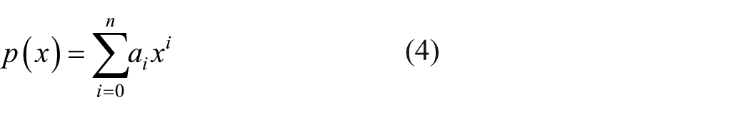
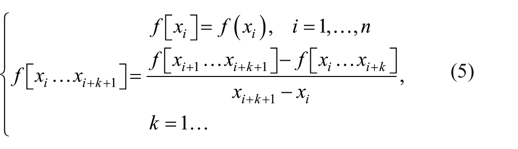
The polynomial $p (x)$ can be computed using the divided differences.

Definition 1

Let f be a function defined in real distinct points xi : i=1,…,n. The divided differences are defined in a recurrent manner as follows

{\begin{matrix} f [x_{i}] = f (x_{i}), i = 1, \dots, n \\ \begin{array}{l} f [x_{i} \dots x_{i + k + 1}] = \frac{f [x_{i + 1} \dots x_{i + k + 1}] - f [x_{i} \dots x_{i + k}]}{x_{i + k + 1} - x_{i}}, \\ k = 1 \dots \end{array} \end{matrix}

(5)

Then, the following proposition comes.

Proposition 1

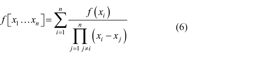
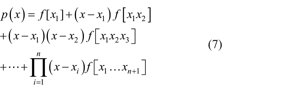
f [x_{1} \dots x_{n}] = \sum_{i = 1}^{n} \frac{f (x_{i})}{\prod_{j = 1 j \neq i}^{n} (x_{i} - x_{j})}

(6)

The following theorem (Newton form) allows to construct the interpolation polynomial using the divided differences.

Theorem 2

The interpolation polynomial $p (x)$ of degree minus or equal to n in points $x_{1}, x_{2}, \dots, x_{n + 1}$ is expressed in the Newton basis as

\begin{array}{l} p (x) = f [x_{1}] + (x - x_{1}) f [x_{1} x_{2}] \\ + (x - x_{1}) (x - x_{2}) f [x_{1} x_{2} x_{3}] \\ + \dots + \prod_{i = 1}^{n} (x - x_{i}) f [x_{1} \dots x_{n + 1}] \end{array}

(7)

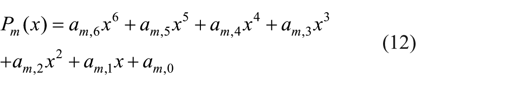
In each direction in the V₂₄ mask (Figure 3), we have seven points (pixels) which will be interpolated by a polynomial of power minus or equal to 6.

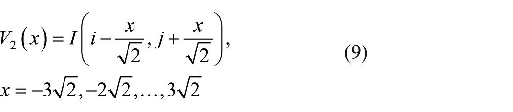
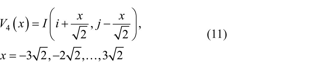
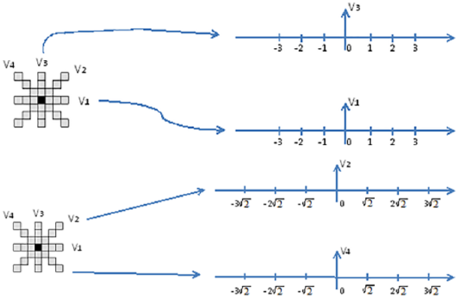
To preserve the pixel dispersion properties (mainly distances between pixels), we use for directions 0 and $π / 2$ (i.e. the horizontal and vertical directions) a unit step between pixels and for the oblique directions $\sqrt{2}$ step as shown in Figure 5.

Figure 5.

Definition of the steps and the corresponding interpolating points with respect to the mask directions for each pixel.

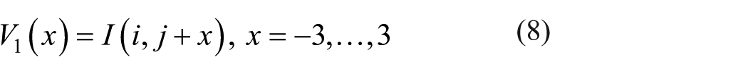
Functions V₁, V₂, V₃, and V₄ are defined for each pixel I(i, j) as follows

V_{1} (x) = I (i, j + x), x = - 3, \dots, 3

(8)

\begin{array}{l} V_{2} (x) = I (i - \frac{x}{\sqrt{2}}, j + \frac{x}{\sqrt{2}}), \\ x = - 3 \sqrt{2}, - 2 \sqrt{2}, \dots, 3 \sqrt{2} \end{array}

(9)

V_{3} (x) = I (i + x, j), x = - 3, \dots, 3

(10)

\begin{array}{l} V_{4} (x) = I (i + \frac{x}{\sqrt{2}}, j - \frac{x}{\sqrt{2}}), \\ x = - 3 \sqrt{2}, - 2 \sqrt{2}, \dots, 3 \sqrt{2} \end{array}

(11)

Let $P_{m} (x)$ be the interpolation polynomial associated with $V_{m} (x)$ for $m = 1, \dots, 4$ . We define $P_{m} (x)$ for the pixel I(i, j) as

\begin{array}{l} P_{m} (x) = a_{m, 6} x^{6} + a_{m, 5} x^{5} + a_{m, 4} x^{4} + a_{m, 3} x^{3} \\ + a_{m, 2} x^{2} + a_{m, 1} x + a_{m, 0} \end{array}

(12)

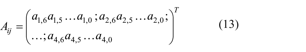
Consequently, each pixel will be characterized, with respect to its neighbors, by 28 coefficients. Let us define for a pixel I(i, j) the interpolation polynomial coefficient vector of length 28 as

A_{i j} = {(\begin{array}{l} a_{1, 6} a_{1, 5} \dots a_{1, 0}; a_{2, 6} a_{2, 5} \dots a_{2, 0}; \\ \dots; a_{4, 6} a_{4, 5} \dots a_{4, 0} \end{array})}^{T}

(13)

For quick simulations and tests, we provided in Appendix 2 the mathematical expressions of the interpolating polynomial coefficients. For textures having some regular regions, there will be many redundant information when scanning the whole of the image. This observation helps at removing repetitive feature vectors and then reducing the number of the learning features for each texture. This will be very useful for the real-time implementation in a further work. In the following, the MLP as well as the learning algorithm are presented, and then, the simulation approach and the generalization results are given.

MLP description

The first step to use a neural network consists in preparing the learning database. Hence, the learning dataset must be formed with two types of feature vectors, namely, one type with defect-free regions and another type with multiple defects.

The neural network architecture is given in Figure 6. It is a fully connected feedforward neural network based on the connection of many single neurons as given in Figure 7.

Figure 6.

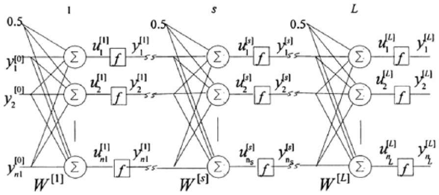
Fully connected multi-layer perceptron.

Figure 7.

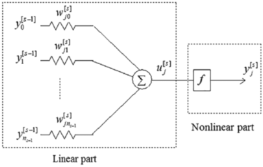
A model for a single neuron (perceptron) in an MLP.

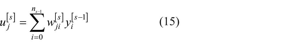
The subscript “j” stands for the number of the neuron in the network, while “s” is the number of the corresponding layer. Each layer consists of $n_{s}$ neurons $(n_{s} : ⤢ 1, \dots, L)$ and $n_{s - 1} + 1$ inputs. The first input of each layer is the bias input (typically 1). The first layer with $n_{0} + 1$ inputs is the input layer. The Lth layer with $n_{L}$ nodes is the output layer. For any neuron “j” in a layer “s,” the nonlinear output signal is defined by

y_{j}^{[s]} = g (u_{j}^{[s]})

(14)

$u_{j}^{[s]}$ is the linear output signal and g is an activation function assumed to be differentiable over ℜ

u_{j}^{[s]} = \sum_{i = 0}^{n_{s - 1}} w_{j i}^{[s]} y_{i}^{[s - 1]}

(15)

The learning algorithm used in this work is the modified backpropagation algorithm presented in Abid et al.²⁰ The major advantage of this algorithm lies in its rapidity of convergence for a quite small modification in the updating equations with respect to the standard backpropagation algorithm. It is based on the optimization of a cost function written as sum of the linear and the nonlinear errors of the output neurons.

The cost function (optimization criterion) is given by equation (16)

E = \sum_{p = 1}^{N} E_{p}

(16)

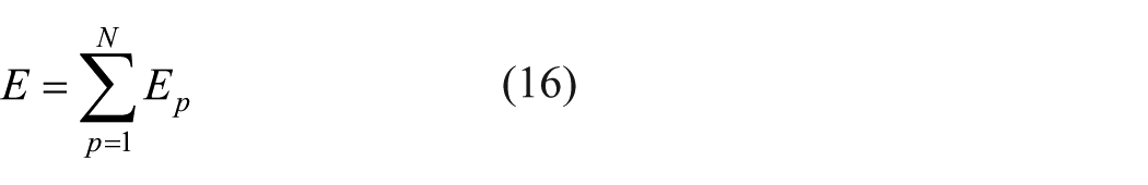
where E_p stands for the sum of the output squared errors for the pth pattern

E_{p} = \frac{1}{2} \sum_{j = 1}^{n_{L}} ({(e_{j}^{[L]})}^{2} + {(l e_{j}^{[L]})}^{2})

(17)

and $e_{j}^{[L]}$ and $l e_{j}^{[L]}$ are the nonlinear and the linear errors of the jth output unit, respectively, and they are given by

e_{j}^{[L]} = d_{j}^{[L]} - y_{j}^{[L]}

(18)

l e_{j}^{[L]} = l d_{j}^{[L]} - u_{j}^{[L]}

(19)

where $d_{j}^{[L]}$ and $y_{j}^{[L]}$ are the desired and the current output signals, respectively, and $l d_{j}^{[L]}$ is the linear desired output obtained by inverting the activation function

l d_{j}^{[L]} = g^{- 1} (d_{j}^{[L]})

(20)

The different steps of the modified backpropagation algorithm are given in Appendix 3; for more details, see Abid et al.²⁰

Simulations

Database presentation

The database of images serving as benchmarks is provided by “PARTNER TEXTILE” company. It consists of mainly 76 images (256 × 256 pixels), having various fabric defects; 50 images are used for the training phase (about two-third of the dataset), and the other 26 are used for test. A summary of some fabric defect types used in this study and their related reasons for appearing are well described in a previous work.²¹ Figure 8 gives some of these defects.

Figure 8.

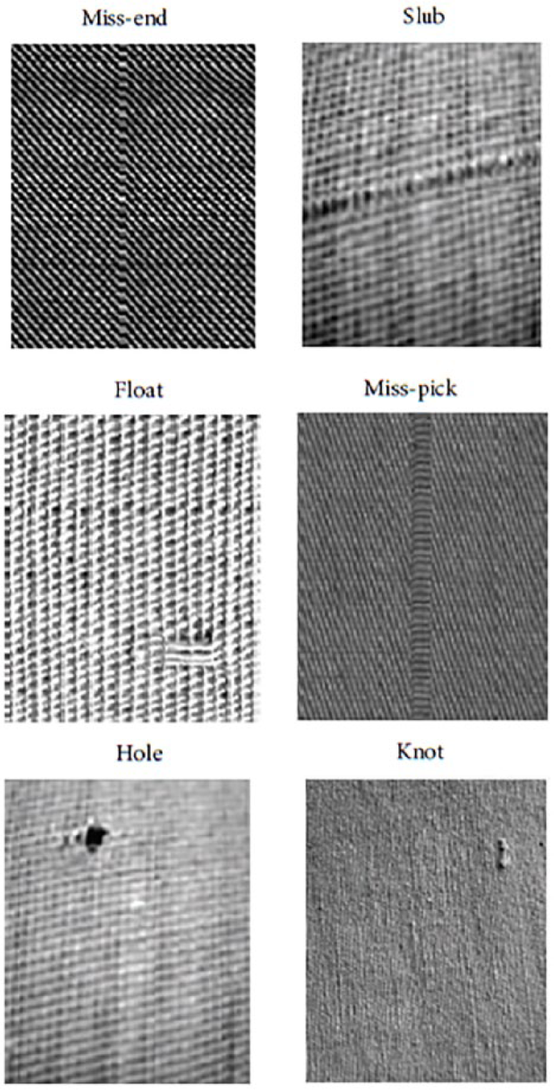
Some of fabric defect caused by a knitting machine.

Simulation description and results

All simulations were performed on personal computer (Intel Core i5-4210U CPU at 1.70 GHz, 2.40 GHz and 6Go of RAM). All programs were tested first in MATLAB language, and then, they were rewritten in C++ language for real-time implementation.

Each image is preprocessed by a median filter to eliminate pixels having high gray levels with respect to their neighborhoods. For each image, we fixed two sets of regions of interest (ROIs), one set corresponds to defect-free regions and the other set corresponds to regions of defects. For each pixel of these regions, we compute the polynomial coefficients and then we propagate them into the network.

In this work, we used a single hidden layer network with 28 inputs (which is the number of the polynomial coefficients) with an additional special input for the bias term, one hidden layer, and one output neuron. The activation function is the sigmoidal one. If the input feature corresponds to a defect-free region, then the desired output is equal to 0.8; otherwise, the network response is equal to 0.2. The different other network parameters are chosen after several simulations to maximize performances of the network (such as the number of the hidden neurons, the learning coefficient, and the sigmoidal slope).

Figure 9 shows the learning curve with respect to the iteration number. The maximum iteration number is chosen equal to 10⁴. In simulations, we tried to avoid the overtraining (i.e. we avoid that the final global error E becomes so small), which may influence the generalization quality due to the big variability of images and shapes of defects.

Figure 9.

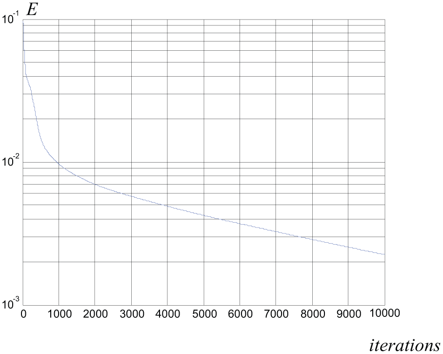
Representation of the learning curve with respect to the iteration number.

In the generalization (test) phase, we used two sets of images. The first contains the images themselves used in the training phase. This is to verify that the network gives good results for regions that were not selected by the ROIs in these images. The second set is formed with new images from the 26 ones that have not been used in the training phase. Figure 10 gives some simulation results for the second set of images.

Figure 10.

Simulation results of the new defect detection scheme: a_i (i = 1–5): the real fabric images, b_i: the neural network responses after binary transformation, and c_i: obtained results after 7 × 7 median filtering.

From the results of the generalization phase shown in Figure 10, one concludes that the new method allows good defect detection for different kinds of defects. Figure 10(c1)–(c3) shows good defect localization while preserving the defect shape. In the following, we shall evaluate the performance of this new approach.

It is important here to give some idea about the acquisition conditions of the different images. Indeed, each knitting machine has been equipped by one light-emitting diode (LED) Batten having the following characteristics: surface-mount device (SMD) LED, 50 W, 3900 Lumens, 1500 mm of length, and 120° lighting angle. Since images are taken while knitting, a progressive scan camera is chosen for each knitting machine. For this purpose, a monochrome digital progressive scan camera is chosen for each machine with time refresh equal to 1/30 s.

Performance evaluation and comparison results

The performance of the proposed approach is treated through the evaluation of the CA known also as the detection success rate. This is later defined as the ratio between the total number of correctly classified samples and the total number of samples

C A = \frac{T P + T N}{T P + T N + F P + F N}

(21)

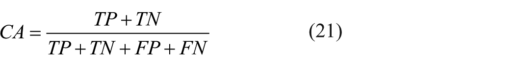
where $C A$ is in general given in percent, TP stands for the test result in the case of defect detection when the defect is really present, TN stands for defect-free detection when the defect is actually absent, FP stands for detection of defect when it does not exist, and FN stands for defect-free detection when a defect actually exists.

For this purpose, we used the 50 images used in the learning phase and the 26 images from the dataset reserved for the generalization phase as mentioned above. In these images, defects are known and well localized to be able to compute exactly the $C A$ rate.

Table 1 gives an evaluation of the CA for the different regions. Recall that in the learning phase, we select the ROIs, but in the generalization phase, we scan the entire image. These results show the very good classification of the new approach. We note that for the 50 images used in the training phase, we do not have 100% CA; this is due to some new regions (not selected by ROIs in the learning phase) which are characterized by an acute dissimilarity with respect to the general aspect of the texture while being considered defect-free regions. The general CA is then given by the mean of the classification accuracies for both training and test images. From Table 1, one notes that CA reaches 99.29%, which can be considered as good classification rate. This shows that the interpolation coefficients can be considered as discriminant features for textures. This fact can be proved through the study of two points:

The uniqueness of the interpolation polynomial for a given set of points $(x_{i}, y_{i})$ .

The slight variation of the related coefficients for a slight variation of $y_{i}$ .

Table 1.

The classification accuracy of the new method for both training and test images.

	Generalization with the training images	Generalization with test images
CA (%)	99.97	98.6
Mean	99.29

Comparison with previous works

The performance of the proposed method is compared with previous works^22–24 and the work of Rebhi et al.²¹ The wavelet transform and morphological mathematics (WT/MM) were used with an MLP to develop a new approach for defect detection in textured images.²² In this work, the Dempster–Shafer theory of evidence was used to combine different evidences and to decrease the value of uncertainty. For the same purpose, Zhang et al.²³ used the principal component analysis (PCA) of a matrix formed with the gray level of each pixel and a radial basis function (RBF) neural network (PCA/RBF). The obtained method reaches a CA of about 83.4%. Qiuping et al.²⁴ used the Gabor filter and sparse coding (GF/SC) to detect defects in twill, plain, gingham, and striped fabric. An accuracy rate around 93% is reached. In this section, we give furthermore a comparison between the proposed approach (polynomial interpolation coefficients with MLP denoted (PIC/MLP)) and our previous work in Rebhi et al.²¹ where we used the local homogeneity analysis and the discrete cosine transform (LHA/DCT) to develop an efficient fabric defect detection algorithm. Table 2 summarizes simulation results of these methods by giving their CA. One notes that these results may lightly vary with the parameters of each method and the images of textures and fabrics although we tried in all simulations to choose the best practical parameters with the aim to maximize the performance of each algorithm.

Table 2.

Comparison of the classification accuracy of the proposed method with respect to several existing ones.

Based method	Classification accuracy (CA, %)
WT/MM	89.48
PCA/RBF	83.4
GF/SC	93
LHA/DCT	97.5
The proposed method PIC/MLP	99.29

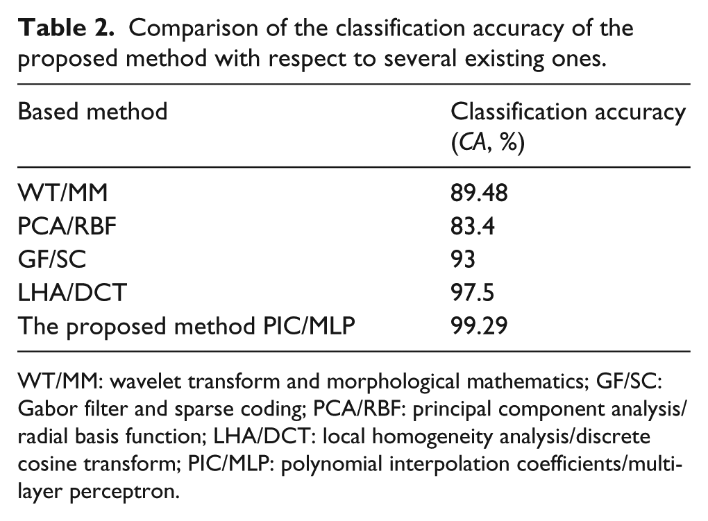
WT/MM: wavelet transform and morphological mathematics; GF/SC: Gabor filter and sparse coding; PCA/RBF: principal component analysis/radial basis function; LHA/DCT: local homogeneity analysis/discrete cosine transform; PIC/MLP: polynomial interpolation coefficients/multilayer perceptron.

Conclusion and perspectives

In this work, we proposed a new method for defect detection in fabrics. This method provides good detection and localization of different types of defects. The CA reaches about 99% for the set of images provided by the company. This rate shows the superiority of the method with respect to several other methods. It is important to note that the proposed approach can be applied for plain fabrics as well as for printed fabrics. Nevertheless, for black colored fabrics, the method may not be suitable in this presented form, and other preprocessing operations must be applied such as histogram translation and/or contrast enhancement. The implementation of this new algorithm in the production line of “PARTNER TEXTILE” company imposes moreover several simplifications which will be presented in a further work.

Footnotes

Appendix 1

Appendix 2

Appendix 3 Acknowledgements

The authors would like to thank Mr Mohamed Ali Derbel, Manager of the “PARTNER TEXTILE,” for the opportunity he offered us to work in this company allowing us to see closely the real problems that the engineer may encounter, for the instructive discussion, and for the database he provided.

Declaration of conflicting interests

The author(s) declared no potential conflicts of interest with respect to the research, authorship, and/or publication of this article.

Funding

The author(s) received no financial support for the research, authorship, and/or publication of this article.

References

Khandelwal

Gautam

PK.

Mechanical part surface defect detection using crack extraction approach. Int J Comput Appl 2014; 100(18): 13–17.

Arjun

Mirnalinee

TT.

Machine parts recognition and defect detection in automated assembly systems using computer vision techniques. Rev Téc Ing Univ Zulia 2016; 39(1): 71–80.

Hegde

Sanjana

Soniya

et al . Quality management of mechanical parts using image processing. Int J Comput Technol Appl 2017; 8(2): 253–256.

Ibrahim

Syed Abu Bakar

SAR

Mokji

et al . A printed circuit board inspection system with defect classification capability. Int J Innov Manag Inf Prod 2012; 3(1): 82–87.

Takada

Shiina

Usami

et al . Defect detection and classification of electronic circuit boards using keypoint extraction and CNN features. In: The ninth international conferences on pervasive patterns and applications (PATTERNS), Athens, 19–23 February 2017.

Mursalin

Eishita

Islam

AR.

Fabric defect inspection system using neural network and microcontroller. J Theor Appl Inform Tech 2008; 4: 560–570.

Ghazvini

Monadjemi

Movahhedinia

et al . Defect detection of tiles using 2D-wavelet transform and statistical features. World Acad Sci Eng Technol 2009; 37: 901–904.

Conners

McMillin

Lin

Identifying and locating surface defects in wood: part of an automated lumber processing system. IEEE T Pattern Anal 1983; 5(6): 573–583.

Zhu

Conners

Araman

. CT image sequence processing for wood defect recognition. In: Proceedings of the IEEE 23rd southeastern symposium on system theory, Columbia, SC, 10–12 March 1991, pp. 75–79. New York: IEEE.

10.

Boukouvalas

Color grading of randomly textured ceramic tiles using color histograms. IEEE T Ind Electron 1999; 46(1): 219–226.

11.

Wiltschi

Pinz

Lindeberg

Automatic assessment scheme for steel quality inspection. Mach Vision Appl 2000; 12(3): 113–128.

12.

https://tn.kompass.com/c/partner-textile/tn592069/

13.

Latif-Amet

Ertuzun

Ercil

An efficient method for texture defect detection: sub-band domain co-occurrence matrices. Image Vision Comput 2000; 18(6): 543–553.

14.

Kumar

Pang

GKH

. Fabric defect segmentation using multichannel blob detectors. Opt Eng 2000; 39(12): 3176–3190.

15.

Hamid

Alireza

Esmaeil

. Defect detection in textiles using morphological analysis of optimal Gabor wavelet. In: Proceedings of the international conference on computer and automation engineering (ICCAE’09), Bangkok, Thailand, 8–10 March 2009, pp. 26–30. New York: IEEE.

16.

Bodnarova

Bennamoun

Latham

Optimal Gabor filters for textile flaw detection. Pattern Recogn 2002; 35(12): 2973–2991.

17.

Kumar

Neural network based detection of local textile defects. Pattern Recogn 2003; 36(7): 1645–1659.

18.

Huang

Chen

I-C.

Neural-fuzzy classification for fabric defects. Text Res J 2001; 71(3): 220–224.

19.

Kumar

Pang

GKH

. Defect detection in textured materials using Gabor filters. IEEE T Ind Appl 2002; 38(2): 425–440.

20.

Abid

Fnaiech

Najim

A fast feed-forward training algorithm using a modified form of the standard back-propagation algorithm. IEEE T Neural Networ 2001; 12: 424–430.

21.

Rebhi

Benmhammed

Abid

et al . Fabric defect detection using local homogeneity analysis and neural network. J Photon 2015; 2015: 376163.

22.

Tabassian

Ghaderi

Ebrahimpour

Knitted fabric defect classification for uncertain labels based on Dempster-Shafer theory of evidence. Expert Syst Appl 2011; 38(5): 5259–5267.

23.

Zhang

Fabric defect classification using radial basis function network. Pattern Recogn Lett 2010; 31(13): 2033–2042.

24.

Qiuping

Minyuan

Jie

et al . Fabric defect detection via small scale over-complete basis set. Text Res J 2014; 84(15): 1634–1649.

Texture defect detection by using polynomial interpolation and multilayer perceptron

Abstract

Keywords

Introduction

New defect detection scheme

Newton form of the interpolating polynomial and its application to the V24 neighborhood

Theorem 1

Definition 1

Proposition 1

Theorem 2

MLP description

Simulations

Database presentation

Simulation description and results

Performance evaluation and comparison results

Comparison with previous works

Conclusion and perspectives

Footnotes

Appendix 1

Appendix 2

Appendix 3

Acknowledgements

Declaration of conflicting interests

Funding

References

Newton form of the interpolating polynomial and its application to the V₂₄ neighborhood