Wind energy resource assessment for Suva,Fiji,with accurate Weibull parameters

Abstract

Abstract

Wind resource assessment is carried out for Suva, the capital of the Republic of Fiji Islands. The wind speeds at 34 m and 20 m above ground level, wind direction, atmospheric pressure, and temperature were measured for more than five years and were statistically analyzed. The daily, monthly, yearly, and seasonal averages were estimated. For the site, the overall average wind speed at 34 m above ground level is found to be 5.18 m/s. The occurrence of effective wind (between the cut-in and cut-off wind speeds of the selected turbine) is predominantly from the east. An effective wind speed of 74.175% was recorded which can be used for power generation. The turbulence intensity and wind shear coefficient are estimated. The site’s overall turbulence intensities are 12.5% and 13.72% at 34 m and 20 m above ground level, respectively. The diurnal wind shear correlated with the temperature variation very well. The overall and seasonal wind distributions are analyzed, which shows that the wind speed in Suva is mostly between 3 m/s and 9 m/s although the winter season has higher wind speeds. The Weibull parameters and the wind power density were found using 10 different methods. The wind power density is estimated to be 159 W/m² using the best method, which is found to be the empirical method of Justus. A high-resolution map around the site is digitized and the wind power density resource map is generated using wind atlas analysis and application program. From the wind atlas analysis and application program analysis, it is seen that Suva has high potential for power generation. Five possible locations are selected for installing wind turbines and the annual energy production is estimated using wind atlas analysis and application program. The total annual energy production from the five sites is 1950 MWh. The average capacity factor of the five turbines is 17%. An economic analysis is performed which showed a payback period of 10.83 years.

Introduction

Renewable sources of energy are becoming increasingly popular throughout the world. Some of the common renewable energy sources being utilized are wind, solar, and hydro. Some benefits of wind energy are that it is the cleanest source of energy and reduces the cost of buying fossil fuels which are expensive and are causing major problems to the environment. To retrieve these fossil fuels, the cost is high as well as this is a finite source of energy which means it will eventually end (Alrikabi, 2014: 61–64). Fossil fuels produce harmful gases such as carbon monoxide and carbon dioxide which lead to harmful effects like global warming (Shahzad, 2012: 16–19). Renewable sources of energy are used to mitigate the greenhouse gas emission and reduce global warming (Panwar et al., 2011). The use of fossil fuels has helped the developing countries to develop faster but with harmful effects (Panwar et al., 2011). One of the effects is the sea level rise near the islands of Tuvalu where the water comes onshore during high tides. To ensure that the source is effective, efficient, and a clean source of energy, an energy assessment needs to be carried out. The wind resource assessment will help researchers to determine the perfect location to set up the wind turbines through the estimation of the wind energy potential of the investigated sites.

A number of articles have been published on wind resource assessment. The major component of wind resource assessment is the estimation of wind power potential for a site before a decision on installing wind turbines can be made. Though many researchers have carried out wind resource assessment, the wind energy potential varies from place to place. The wind speed and the wind direction vary, and as a result, the Weibull parameters for each site will also differ. The method that gives accurate Weibull parameters will also differ from place to place. Fazelpour et al. (2017) carried out a wind resource assessment at four locations in Iran and found that the best sites based on the annual mean wind speeds were Zabol and Zahak which have wind speeds of 5.59 m/s and 5.48 m/s, respectively, at 10 m AGL (above ground level). In the analysis, they just used the empirical method of Justus (EMJ) to determine the k and A parameters. Zabol also had the highest annual mean wind power density (WPD) of 284.97 W/m². Ahmad et al. (2003) statistically analyzed one year of wind data for four sites in Malaysia. From the analysis, it was found that wind power generation would be more efficient during the northeast monsoon season in which wind speeds are higher. To find the k and A parameters, they used three different methods. The best Weibull parameter estimation method for the sites in Malaysia, from the study, was the maximum likelihood method (ML). Bassyouni et al. (2015) did a statistical analysis for 10 years of wind data for a site in Jeddah, Saudi Arabia. It was found from the study that the city had lower mean wind speed of 2.86–3.87 m/s at 10 m AGL; thus, it was concluded that small wind turbines can be installed for the analyzed sites. The WPD was also less, ranging between 42.86 W/m² and 83.78 W/m² which is more favorable for smaller wind turbines. Dabbaghiyan et al. (2015) did wind resource assessment with one year data collected at heights of 10 m, 30 m, and 40 m AGL for the sites at Bushehr, Iran. The important conclusions made were that the site which was proven to be the best was Bord Khun, because this site showed the best annual mean power densities of 115–175 W/m². Katinas et al. (2017) statistically analyzed the wind data for Lithuania. In the study, eight different Weibull parameter estimation methods were used. From the eight methods, the most accurate method was found to be the ML for the site. The wind speeds for most of the sites in Lithuania are around 4 m/s at 10 m AGL; thus, it was recommended that wind power generation is possible for this area. A study done in Hong Kong by Shu et al. (2015) showed that different Weibull parameter estimation methods are unique for each of the analyzed sites. In the analysis, three different methods were used to find the Weibull parameters. From their analysis, it was noted that the Weibull parameters differ in seasons. During autumn the shape parameter was estimated to be the highest, while for summer, the shape parameter was the lowest. Soulouknga et al. (2018) performed a statistical analysis for the site in Chad and made recommendations on selecting the cost-effective wind turbines for the site. In their analysis, they used 18 years of data collected at a height of 10 m AGL. The maximum monthly wind speed was recorded in January, while the minimum monthly wind speed was recorded in August having speeds of 4 m/s and 2.2 m/s, respectively. To find the Weibull parameters, six different Weibull approximation methods were used. The average annual power density was calculated as 343.31 W/m². Based on the WPD and the wind speed, the Saharan zone area was classified as class 1, where the WPD $\le$ 100 W/m² and the wind speed $\le$ 4.4 m/s based on the article by Azad et al. (2014b). According to Mohammadi et al. (2016), the wind characteristics play an important role in determining the best Weibull parameter estimation method for a site. From the six Weibull parameter estimation methods used, EMJ was found to be the best method of Weibull approximation for the Lethbridge A and Waterton Park Gate sites and energy pattern factor method (EPF) was found to be the best method for Edmonton and Grande Prairie sites. One of the findings was that EMJ and empirical method of Lysen (EML) are very close in terms of the efficiency but EMJ has a better performance. Another study that confirms that different sites need to find and use different Weibull parameter estimation methods was performed by Werapun et al. (2015) for Phangan Island, Thailand. It was concluded that the EPF was very effective in calculating the Weibull parameters from the five different methods used. According to Azad et al. (2014a), the most effective Weibull parameter estimation for Hatiya Island was the moments methods (MOs) out of the four methods that were used in the study. It was also found that the winds in Hatiya were higher ranging between 2.62 m/s and 14.01 m/s. It was concluded that the site has enough potential which can drive small wind turbines for the generation of electricity. Rocha et al. (2012) statistically analyzed the performance of seven different methods of Weibull parameters for the wind energy generation at sites in Brazil using 20 months of wind data. The best method was the equivalent energy method based on the performance analysis. It was noted that when there is a lower standard deviation of the wind speeds, there is an increase in the trend of the curve adjustments of the wind speed histograms.

The present work is carried out to study the wind characteristic and to estimate the wind energy potential of the Suva site using the measured data. The wind data are first analyzed in terms of the averages. The wind shear is then correlated to the temperature. The turbulence intensity (TI) is calculated to know how effective the wind speed is on the site. The predominant wind direction is shown through the wind rose plots. Using the performance analysis, the best Weibull parameter estimation method is obtained from the 10 different methods used to find the k and A parameters with the WPD of the site. The annual energy production (AEP) is calculated and an economic analysis is carried out to determine the payback period of installing 275 kW Vergnet wind turbines.

Data and methods

A detailed wind analysis is carried out in order to implement the generation of power for Suva, Fiji Islands. This analysis will help in finding the perfect location to set up the turbines to harvest the maximum wind energy. The selection of wind measurement site, installation of wind measurement towers and instrumentations, collection and validation of the data, methods of estimating Weibull parameters, and the methods of analyzing the performance of different methods are described in the following sections.

Wind measurement site

The site chosen for the wind data analysis for the present work is located at the Statham Campus, the University of the South Pacific, Suva, Fiji. Fiji is one of the developing island nations in the South Pacific with a population of approximately 900,000. Fiji has a land area of approximately 18,274 km² and has approximately 332 islands of which the two main islands are Viti Levu and Vanua Levu. Viti Levu has the highest population of which Suva is the most populous urban center. Suva is the capital of Fiji and is also the political, economic, and the cultural center. The site location selected has one side facing directly the open sea, while the other side is land. The site is very close to the shoreline with a distance of approximately 40 m. Suva city is in the province of Rewa and is located in one of the two largest islands of Fiji, Viti Levu. Suva city is the capital of Fiji which is a heavily populated area of Fiji with about 100,000 people. The geographic location of the site is 18° 8' 38.688'' South 178° 27′ 25.7508″ East. Figure 1 shows the location of the site where the measurements were performed. The total land area of Suva city is about 44 km². Suva is known to have the tropical rainforest climate since this city has no true dry season because it rains throughout the year with more rain from November to April. The measurement period of the wind data was from October 2012 to April 2018.

Figure 1.

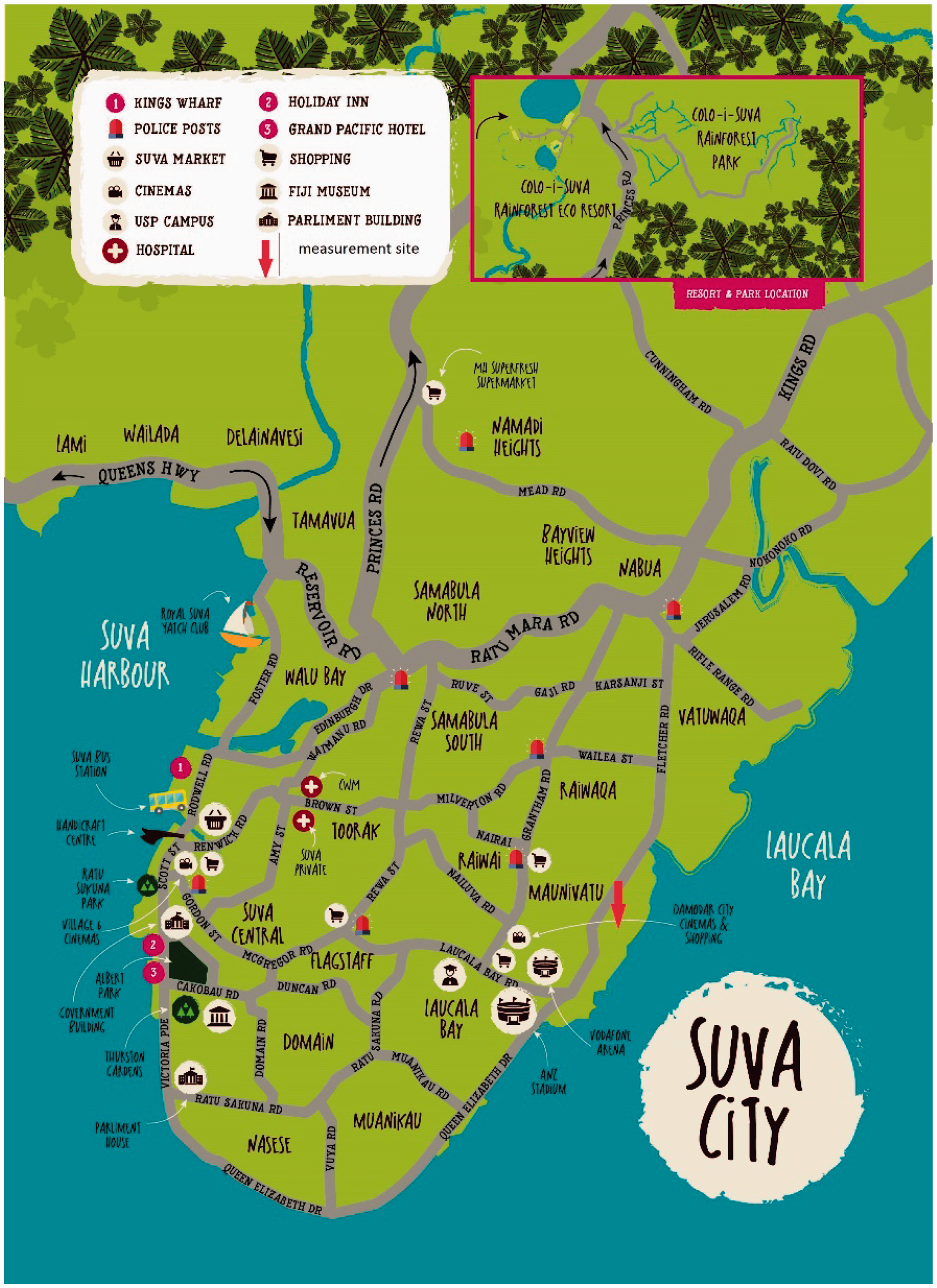
Map of Suva showing the measurement location (Resort C-i-SRE, 2018).

Fiji’s main electricity provider is Energy Fiji Limited (EFL), which was known as Fiji Electricity Authority till recently. Fiji’s electrical power generation is comprised of hydro generation, diesel generation, and wind generation. A total of 237 MW of electricity is produced throughout the country. In Viti Levu, approximately 212 MW of electricity is produced of which 92 MW is from diesel generation and 120 MW is from renewables (EFL).

Measurement tower and instrumentations

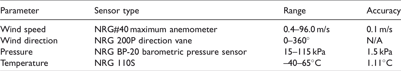
The measurement tower is of 34 m height and is a NRG system tower. Such NRG towers are used all around the globe. There is a NRG data-logger, SymphoniePlus3, installed on the tower. This NRG data-logger has a total of seven sensors. These sensors measure the wind speed, temperature, atmospheric pressure, rainfall, solar insolation, humidity, and wind direction. The data are recorded every 10 min on the NRG data-logger’s SD card. There is also a GSM based transfer of data. The data from the NRG data-logger can be extracted directly from the SD card or can be transferred via GSM network to the data-bank which is located at the ICT centre of USP at Laucala Campus. The accuracy of the anemometers is 0.1 m/s and has a range between 0.4 m/s and 25 m/s. The wind vane was aligned to the true north and placed at 30 m height. A temperature sensor was mounted on the tower to get the measurements of temperature. For obtaining accurate values of temperature, a circular six radiation shield was provided around the sensor. The specifications of each sensor are shown in Table 1.

Table 1.

Specifications of the measurement sensors (Aukitino et al. 2017).

Parameter	Sensor type	Range	Accuracy
Wind speed	NRG#40 maximum anemometer	0.4–96.0 m/s	0.1 m/s
Wind direction	NRG 200P direction vane	0–360°	N/A
Pressure	NRG BP-20 barometric pressure sensor	15–115 kPa	1.5 kPa
Temperature	NRG 110S	–40–65°C	1.11°C

There were some uncertainties which had to be taken into account. Some of the uncertainties were the calibration errors, the terrain of the site that was used, and the dynamic overspeeding, the error that was produced due to the wind shear and the inflow angle. This research is based on averages of very large dataset samples; thus, it may be stated that each parameter tested has an error which is <1%.

Data collection and validation

Five years of data was obtained from the data-logger by extracting the raw data from the installed SD card. The raw data were then processed to obtain the processed data in excel format. The five years of data were first validated for processing. To start with, the first validation process was the range test. This was done to check that the range of the obtained data did not fall out of the given range of the anemometer. The given range of the anemometer for the mean wind speed was 0.4–96.0 m/s. The obtained data range for the 34 m AGL was 0.4–29.5 m/s and at 20 m, it was 0.4–27.6 m/s. The recorded maximum wind speed at 34 m AGL and 20 m AGL was 38.2 m/s and 35.1 m/s. The temperature recorded in the time frame was within the given range. The recorded mean 10 min maximum and minimum temperatures were 34.21°C and 17.32°C. The wind speeds measured at 34 m AGL for the entire period from the two anemometers were compared and are shown in Figure 2. The average difference between the mean wind speeds for the two anemometers at 34 m was 0.98%.

Figure 2.

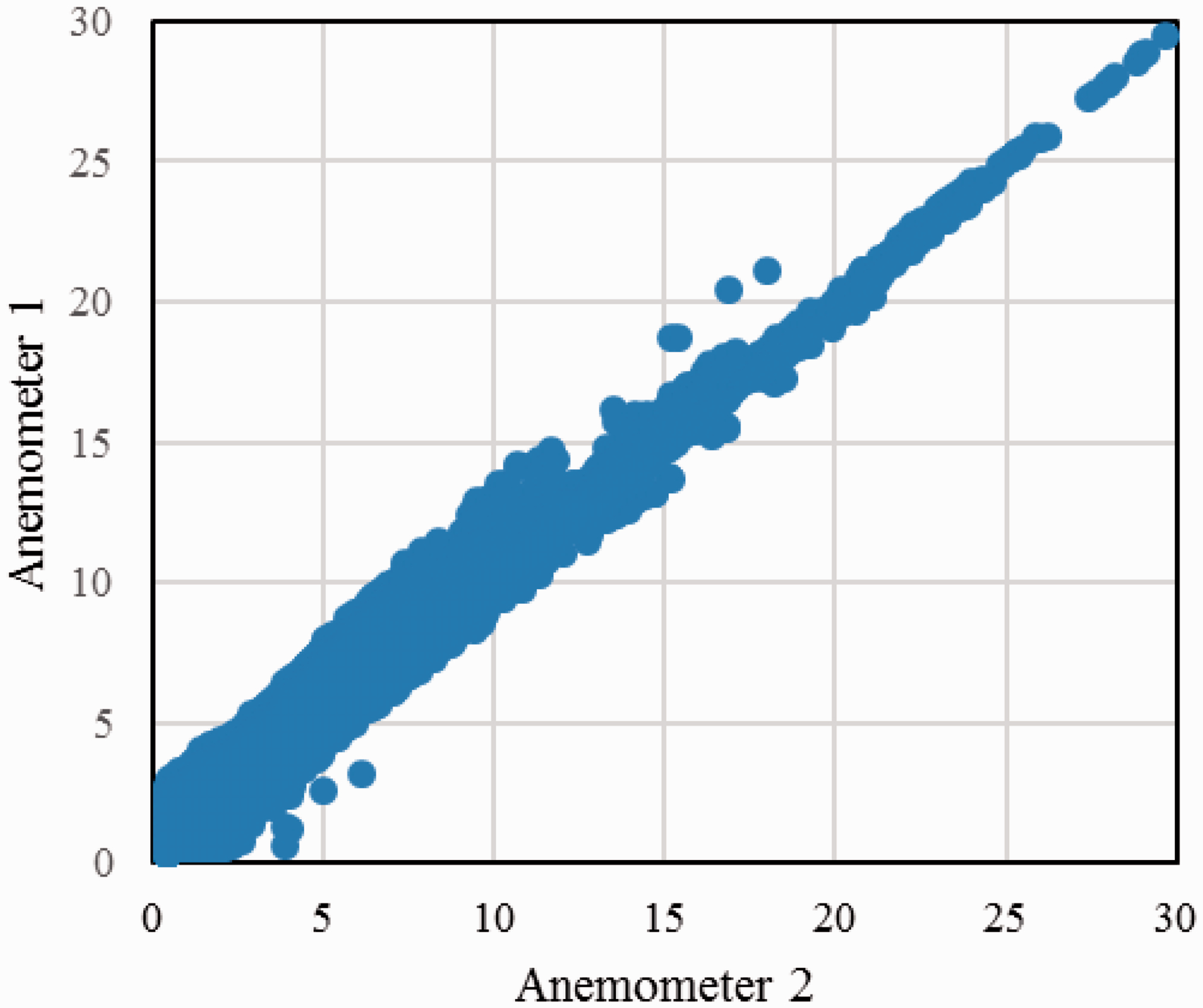
Comparison of wind speeds from the two anemometers installed at 34 m AGL.

Estimation of Weibull parameters

The best Weibull parameters were determined through statistical analysis. The wind speeds are never taken to be negative and are bounded only to one side (Zhang, 2015). Normal distribution could not be used; thus, the best distribution to model the wind speed is the Weibull distribution. In Weibull distribution, there are two parameters which are adjusted to suit the distribution of the wind. The Weibull probability density function is shown in equation (1) which uses the two parameters k and A:

$$f(U)=\frac{k}{A}{\left(\frac{U}{A}\right)}^{k-1}{e}^{-{\left(\frac{U}{A}\right)}^k}$$

(1)

where U is the wind speed, k is the shape factor, and A is the scale factor.

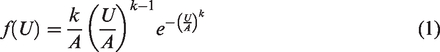
To determine these parameters, there are several methods that have been tried; however, no single method is found to be the best for different sites encouraging further research either from new sites or using new or modified methods. In the present work, 10 different methods were used to find the Weibull parameters. The Weibull parameters that are obtained from the best method are used to find the AEP at the site. The Weibull parameters are found using 10 different methods: the median and quartiles method (MQ), the MO, the EMJ, the EML, the least squares method (LS), the ML, the modified maximum likelihood method (MML), the EPF, the wind atlas analysis and application program (WAsP) method, and method of multi-objective moments (MM). The methods used in the analysis are described below:

MQ

Justus et al. (1978) had found k and A by defining the median wind velocity (U_m) and further the quartiles wind velocities of 25% (U_0.25) and 75% (U_0.75). Equations (2) and (3) are used to determine the values of k and A.

$$k=\frac{\ln \left[\ln (0.25)/\ln (0.75)\right]}{\ln (U_{0.75})/U_{0.25}}\approx \frac{1.573}{\ln (U_{0.75})/U_{0.25})}$$

(2)

$$A=\frac{U_m}{\ln {(2)}^{1/a}}$$

(3)

MO

Justus et al. (1978) also suggested MO. To calculate the k and A values, the standard deviation of the wind speed and the mean wind speeds are used as shown in equations (4) and (5). These equations have been discussed and clarified in several previous works (Chaurasiya et al., 2017, 2018; Rocha et al., 2012).

$$\overline{U}=A\text{Γ}\left(1+\frac{1}{k}\right)$$

(4)

$$\sigma =A{\left[\text{Γ}\left(1+2/k\right)-{\text{Γ}}^2\left(1+1/k\right)\right]}^{1/2}$$

(5)

EMJ

This method was also first used by Justus et al. (1978). According to Mohammadi et al. (2016), the k and A values can be calculated using equations (6) and (7):

$$k={\left[\frac{\sigma }{\overline{U}}\right]}^{-1.086}$$

(6)

$$A=\overline{U}/\text{Γ}\left(1+1/k\right)$$

(7)

EML

This method was introduced by Lysen (1982). This method is a modification of the EMJ. The k value is obtained using equation (6) but the equation of A differs. Equation (8) shows how A is obtained from the value of k (Chaurasiya et al., 2017, 2018).

$$A=\overline{U}{\left(0.568+0.433/k\right)}^{-\frac{1}{k}}$$

(8)

LS

In engineering, this method is one of the most commonly used methods. In this method, the manual probability is plotted using a formalized technique. This method is a linear correlation where two of the variables are assumed. Through some calculations, the Weibull parameters are found. The final k and A parameters are obtained using equations (9) and (10) (Chaurasiya et al., 2017, 2018).

$$k=\frac{n{{\displaystyle \sum }}_{i=1}^n\ln \mathit{Ux}\ln \left[-\ln \left\{1-f\left(U\right)\right\}\right]{{\displaystyle \sum }}_{i=1}^n\ln \mathit{Ux}{{\displaystyle \sum }}_{i=1}^n\ln \left[-\ln \left\{1-F\left(U\right)\right\}\right]}{{{\displaystyle \sum }}_{i=1}^n\ln U^2-{\left\{{{\displaystyle \sum }}_{i=1}^n\ln U\right\}}^2}$$

(9)

$$A=\frac{k{{\displaystyle \sum }}_{i=1}^n\ln U-{{\displaystyle \sum }}_{i=1}^n\ln \left[-\ln \left\{1-F\left(U\right)\right\}\right]}{\mathit{nk}}$$

(10)

ML

“This method uses a likelihood function of the wind speed data in time series format” (Warudkar, V. et al.; Chaurasiya et al., 2017; Saleh et al., 2012). For instance, the values for a random wind dataset (U1, U₂, U₃…U_n) are given and the Weibull probability density function is given. The likelihood function from the given sample L (k, A, U₁, U₂, U₃…U_n) can be stated as in equation (11) (Ahmad et al., 2003; Katinas et al., 2017; Mohammadi et al., 2016; Rocha et al., 2012).

$$L\left(k;\hspace{0.17em}A;U_1;\hspace{0.17em}{U}_2;\hspace{0.17em}{U}_3; . . . . . . U_n\right)= {\displaystyle \prod }_{i=1}^{n}f\left(k,A,U_i\right)$$

(11)

where the function is further simplified to

$$\ln L= {\displaystyle \sum }_{i=1}^n\ln \left[f\left(U_i\right)\right]$$

(12)

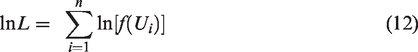
Equation (12) gives rise to the equations for k and A values

$$\frac{\partial \ln L}{\partial k}= 0$$

(13)

$$\frac{\partial \ln L}{\partial A}= 0$$

(14)

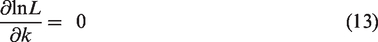
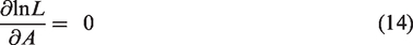
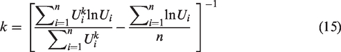
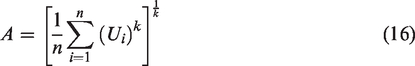
With the help of equations (15) and (16), k and A are formulated

$$k={\left[\frac{{{\displaystyle \sum }}_{i=1}^n{U}_{\mathit{i}}^k\ln U_i}{{{\displaystyle \sum }}_{i=1}^n{U}_{\mathit{i}}^k}-\frac{{{\displaystyle \sum }}_{i=1}^n\ln U_i}{n} \right]}^{-1}$$

(15)

$$A={\left[\frac{1}{n}{\displaystyle \sum }_{i=1}^n{(U_i)}^k\right]}^{\frac{1}{k}}$$

(16)

MML

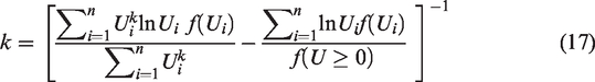
The method is similar to the ML; however, in this method, the wind speed is binned based on the frequency of the wind speed to later find the Weibull parameters. This method involves high-level numerical analysis. Equations (17) and (18) are modified from the ML (Ahmad et al., 2003; Katinas et al., 2017; Mohammadi et al., 2016; Rocha et al., 2012).

$$k={\left[\frac{{{\displaystyle \sum }}_{i=1}^n{U}_{\mathit{i}}^k\ln U_i f\left(U_i\right)}{{{\displaystyle \sum }}_{i=1}^n{U}_{\mathit{i}}^k}-\frac{{{\displaystyle \sum }}_{i=1}^n\ln U_{i}f\left(U_i\right)}{f\left(U\ge 0\right)} \right]}^{-1}$$

(17)

$$A={\left[\frac{1}{f\left(U\ge 0\right)}{\displaystyle \sum }_{i=1}^n{(U_i)}^{k}f\left(U_i\right)\right]}^{\frac{1}{k}}$$

(18)

EPF

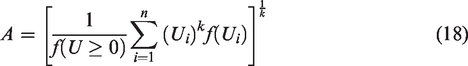
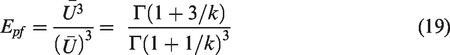
This method is also named as power density method. According to several previous works (Chaurasiya et al., 2017, 2018; Rocha et al., 2012; Zhang, 2015), this method uses the ratio of the cubic wind speed and the cubic of the mean speed of the wind as shown in equation (19).

$$E_{\mathit{pf}}=\frac{\overline{U^3}}{{\left(\overline{U}\right)}^3}= \frac{\Gamma \left(1+3/k\right)}{\Gamma {\left(1+1/k\right)}^3}$$

(19)

where $\overline{U^3}$ represents the mean of the cube of wind speed and ${\left(\overline{U}\right)}^3$ represents the cube of the mean wind speed. After calculating E_pf using equation (19), the Weibull parameters are calculated. The k and A parameters are represented by using equations (20) and (21):

$$k=1+\frac{3.69}{E_{\mathit{pf}}^2}$$

(20)

$$A=\frac{\overline{U}}{\text{Γ}\left(1+1/k\right)}$$

(21)

WAsP

The WAsP software was developed by the RisØ National Laboratory in 1987 for analyzing wind data. This software can be used to calculate the energy yield, wind farm efficiency, wind resource, and turbulence mapping, calculation of wind conditions like mean wind speed, wind shear, ambient turbulence, extreme wind, and wind flow inclination, and also the Weibull parameters, k and A. Version 11 of the WAsP software is used for the present calculations. The WAsP method has the following requirements (Aukitino et al., 2017):

The WAsP method does not directly fit the measured frequency histogram.

The mean power densities from the fitted Weibull distribution should be equal to that of the observed one.

The proportion of values above the mean observed wind speed from the fitted Weibull distribution should be equal to those from the observed distribution.

From these requirements, the equation of wind speed (U) is derived as shown in equation (22):

$$U= \sqrt{\frac{{\sum }_{i=1}^n{U}_i^3}{N\text{Γ}\left(\frac{3}{k}+1\right)}}$$

(22)

From the cumulative distribution function, $F(U)$ , the values of less than $U$ are obtained. Thus, the values that exceed $U$ are represented by $1-F(U)$ . From the last requirement, the proportion of the observed wind speeds that exceed the mean observed wind speed must be determined and we represent it as Z; thus, Z will be

$$Z=1-F(U)$$

(23)

$${\left(\frac{\overline{U}}{\sqrt[3]{\frac{{\sum }_{i=1}^n{U}_i^3}{N\Gamma \left(\frac{3}{k}+1\right)}}}\right)}^k=-\ln (Z)$$

(24)

First Z is calculated from equation (23); then, k is obtained from equation (24).

MM

This method is recently introduced by Usta et al. (2018). This method proposes the squared deviance minimization between the sampling moments and the first three moments. To find the Weibull parameters, the following equation is used:

$${\lambda }_1{\left(A\Gamma \left(1+\frac{1}{k}\right)-\overline{v}\right)}^2+{\lambda }_2\left(A^2\Gamma \left(1+\frac{2}{k}\right)-\overline{v^2}\right)+{\lambda }_3\left(A^3\Gamma \left(1+\frac{3}{k}\right)-\overline{v^3}\right)$$

(25)

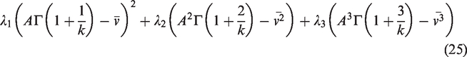
For the ${\lambda }_1$ , ${\lambda }_2$ , and ${\lambda }_3$ it is taken in to consideration that:

$${\lambda }_1+{\lambda }_2+{\lambda }_3=1$$

(26)

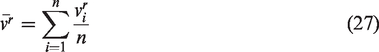
The rth sampled moments are represented by

$$\overline{v^r}={\displaystyle \sum _{i=1}^n\frac{v_{\mathit{i}}^r}{n}}$$

(27)

Performance analysis

To quantify which method is best for finding the Weibull parameters for a location, a quantitative assessment of the model’s performance must be carried out. There are various methods to assessments, some of which are:

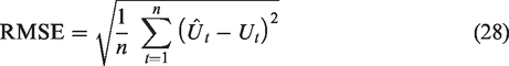
Root mean square error (RMSE)

The RMSE is calculated using equation (28) (Aukitino et al., 2017; Chaurasiya et al., 2017, 2018). The RMSE checks for accuracy of the model by checking the value obtained by the Weibull function and the raw data that have been measured. The lower the RMSE, the better the Weibull distribution. The RMSE will never have a negative value.

$$\text{RMSE}=\sqrt{\frac{1}{n} {\displaystyle \sum }_{t=1}^n{\left({\widehat{U}}_t-U_t\right)}^2}$$

(28)

Coefficient of determination (R²)

It checks the method’s ability to estimate the variables accurately. It is considered that the higher the R², the better the method is. The range of R² is between 0 and 1. Equation (29) shows how the R² is calculated (Chaurasiya et al., 2017, 2018).

$$R^2=\frac{{\sum }_{i=1}^n\left|U_t-{\widehat{U}}_t\right|}{{\sum }_{i=1}^n\left|U_t-{\overline{U}}_t\right|}$$

(29)

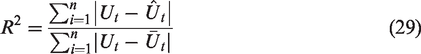
The variables $U_t$ and ${\widehat{U}}_t$ are the actual wind speed and the predicted wind speed, respectively. The t stands for the time (1, 2, 3… n) and the n stands for the number of observations that are made.

Mean absolute error (MAE)

It is a measure of the difference between two continuous variables. The MAE is the average of the absolute errors. The lower the MAE, the better the accuracy. Equation (30) shows how the MAE is estimated (Aukitino et al., 2017).

$$\text{MAE}=\frac{1}{n}{\displaystyle \sum }_{t=1}^n\left|{\widehat{U}}_t-U_t\right|$$

(30)

Mean absolute percentage error (MAPE)

The MAPE calculates the difference between the wind speeds computed using a Weibull function and the measured values. The value for MAPE is calculated using equation (31) (Aukitino et al., 2017; Chaurasiya et al., 2017, 2018):

$$\text{MAPE}=\frac{1}{n}{\displaystyle \sum }_{i=1}^n\left|\frac{{\widehat{U}}_t-U_t}{U_t}\right|\times 100$$

(31)

Coefficient of efficiency (COE)

Another way to check the efficiency of a method is by using the COE. The greater the COE, the better the accuracy of the method (Aukitino et al., 2017).

$$\text{COE}=\frac{{{\displaystyle \sum }}_{i=1}^N{\left({\widehat{U}}_t-\overline{U}\right)}^2}{{{\displaystyle \sum }}_{i=1}^N{\left(U-\overline{U}\right)}^2}$$

(32)

Results and discussion

Wind speed analysis

The results of the wind speed analysis for the site at Suva are presented in this section. The five years continuous data for Suva were analyzed for hourly, daily, monthly, yearly, and seasonally averaged wind speeds. Zhang (2015) used equation (33) to find the mean wind speed.

$$\overline{U}=\frac{1}{n}{\displaystyle \sum }_{i=1}^n{U}_i$$

(33)

where $\overline{U}$ is the averaged wind speed and U_i is the wind speed recorded at constant intervals, i.e. 10 min average for the data under study, and n represents the number of observations and i is the interval at which the data were recorded. The overall average wind speed for 34 m AGL recorded over the assessment period was 5.18 m/s.

Figure 3 represents the averaged daily wind speed for the site at the height of 34 m AGL. The wind speeds are plotted for the entire period of study from October 2012 to April 2018. The averaged daily wind speed ranged between 0.4 m/s and 18.97 m/s. From the daily average analysis, it was observed that the daily averaged maximum wind speed of 18.97 m/s was recorded on the 17th of December in 2012 and the maximum averaged 10 min wind speed of 29.5 m/s was also recorded on the same day. It should be noted that during December 2012, Cyclone Evan affected the site with very high-speed winds. There were at least other 13 cyclones which affected Fiji during the period of study. These cyclones showed higher wind speeds in the results.

Figure 3.

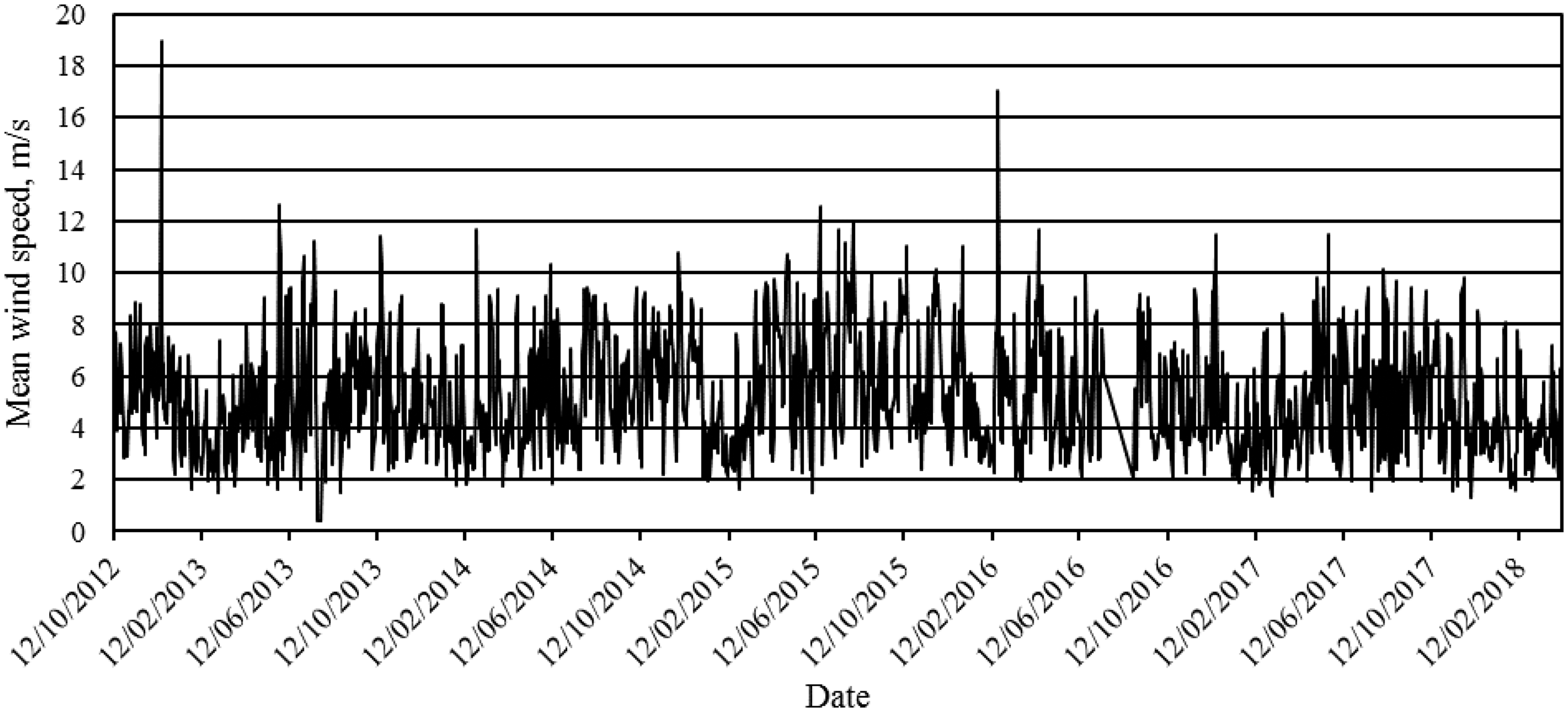
Daily average wind speeds at 34 m AGL for the entire duration of measurements.

The mean of the overall data for every hour was estimated to get the hourly mean of the entire data for 24 h and the result is shown in Figure 4. The wind speed was observed to be higher after midday while lower during the night. At 8 a.m., the mean wind speed is the lowest and starts to increase during the day. The peak is reached at 3 p.m. and then the wind speed starts to decrease through night till 8 a.m. in the morning. From this analysis, it is clear that the site is windier after midday.

Figure 4.

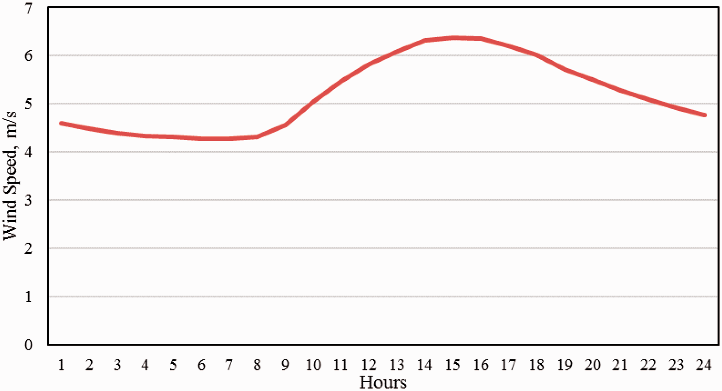
Diurnal variation of wind speed at 34 m AGL for the entire measurement period.

The yearly averaged wind speeds from 2012 to 2018 are shown in Figure 5. From the analysis, the mean wind speed was about 5–6 m/s for most of the years. The annual mean wind speed for 2013 was 4.89 m/s which is lower compared to the other years. Also, during this year, El Nino was observed. “During an El Niño year, weakening winds along the equator lead to warming water surface temperatures that lead to further weakening of the winds” according to Michael McPhaden of NOAA’s Pacific Marine Environmental Laboratory (Mike Carlowicz, 2017). So, from the results, El Niño affected Fiji in 2013 causing lower wind speeds. It should also be noted that for 2018, the data till April 2018 were analyzed, resulting in a lower wind speed in Figure 6. The wind speeds are higher after March, as can be seen below.

Figure 5.

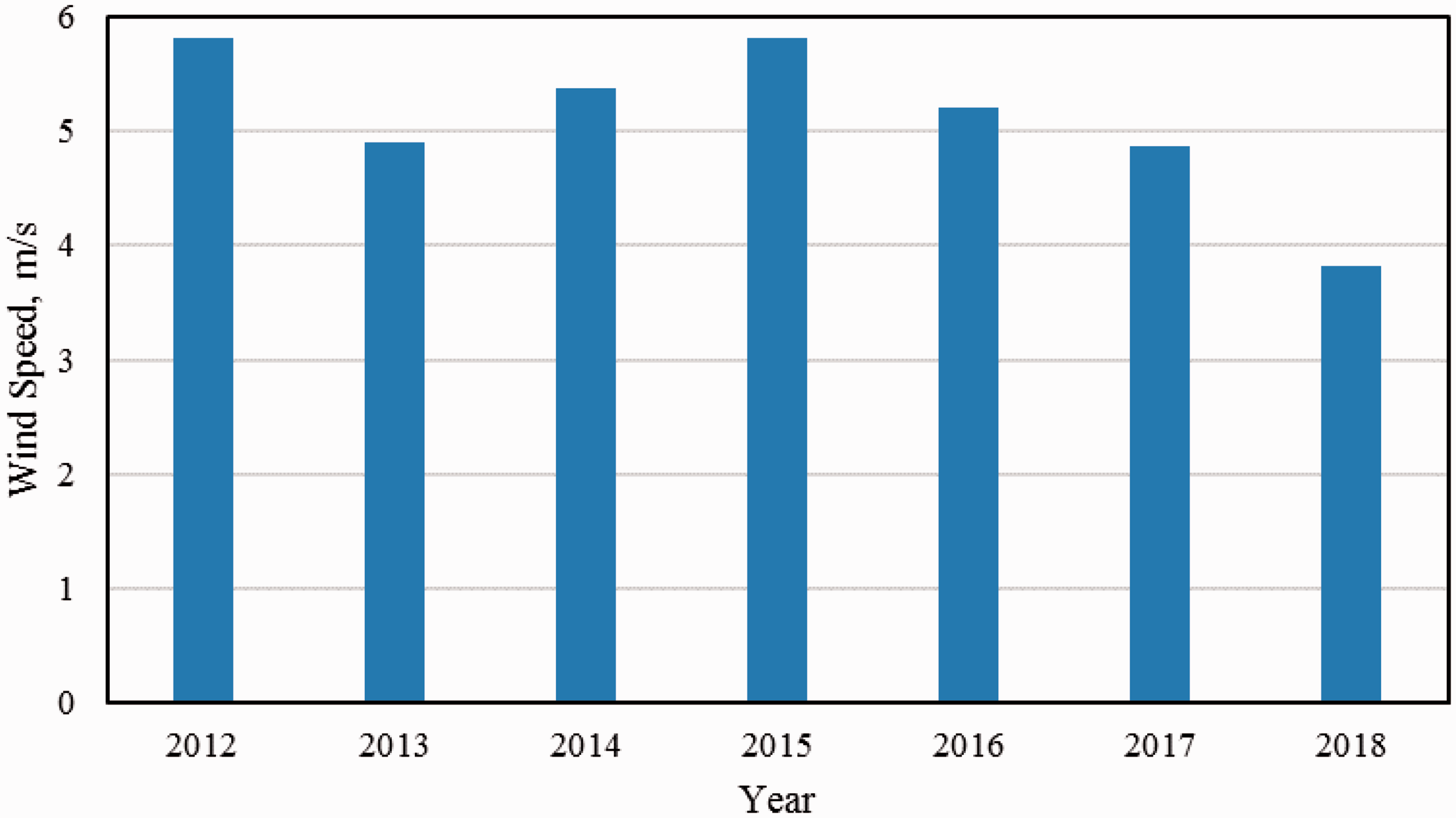
Variation of annual mean wind speed at 34 m AGL for the summarized entire period.

Figure 6.

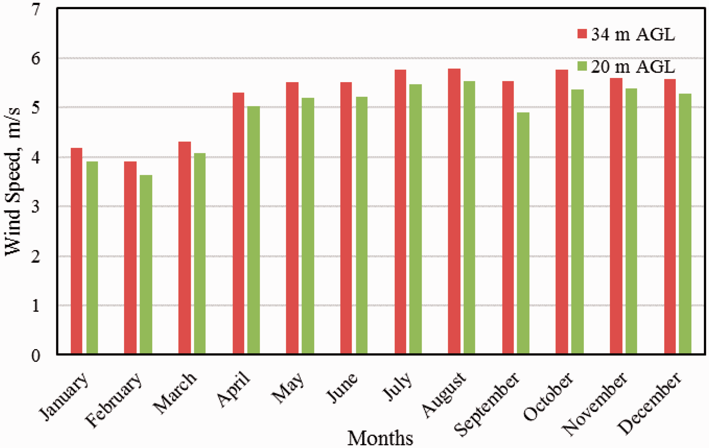
Monthly averaged wind speed at 34 m AGL and 20 m AGL for the summarized entire period.

The overall monthly average wind speed analysis was done and the results are shown in Figure 6. The monthly maximum averaged wind speed of 5.79 m/s was recorded at 34 m AGL and 5.54 m/s was recorded at 20 m AGL, both for the month of August. It can be seen that January, February, and March recorded lower wind speeds compared to other months. While the starting three months recorded around 4 m/s, the rest of the nine months recorded above 5 m/s. These results were then further analyzed by looking at each month for the different years for 34 m AGL as shown in Figure 7. The highest averaged wind speed of 6.88 m/s was recorded for August 2014. It is clearly evident that the wind speeds vary from month to month and also year to year.

Figure 7.

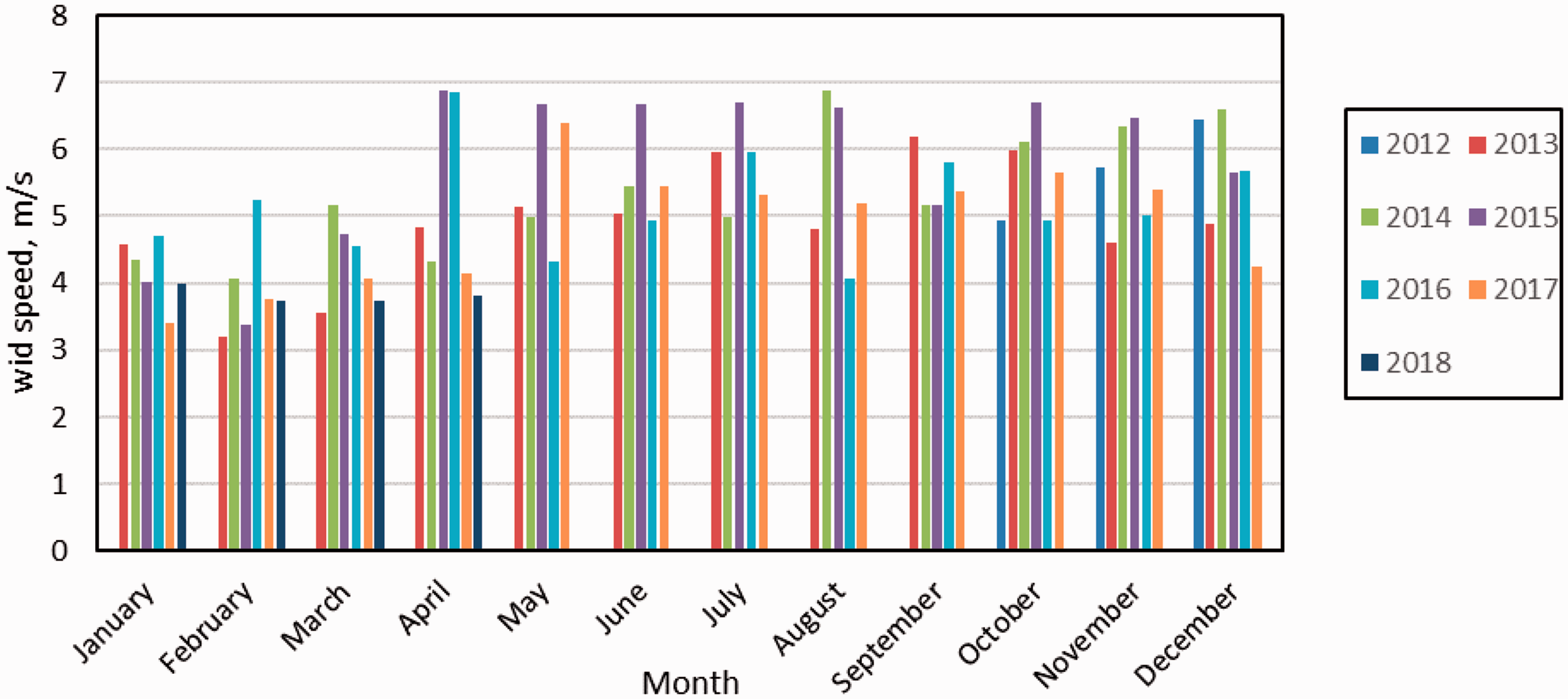
Monthly averaged wind speeds at 34 m AGL for the measurement period.

Fiji has mainly two seasons: summer and a mild winter, also known as wet season and dry season. From the analysis shown in Figure 8, it was observed that the winter months experienced higher winds compared to the summer months. The average wind speed for the winter season was 5.64 m/s, while that for the summer season was 4.81 m/s at 34 m AGL. The same trend was observed at 20 m AGL, the summer averaged 4.55 m/s, while winter had a higher wind speed of 5.28 m/s.

Figure 8.

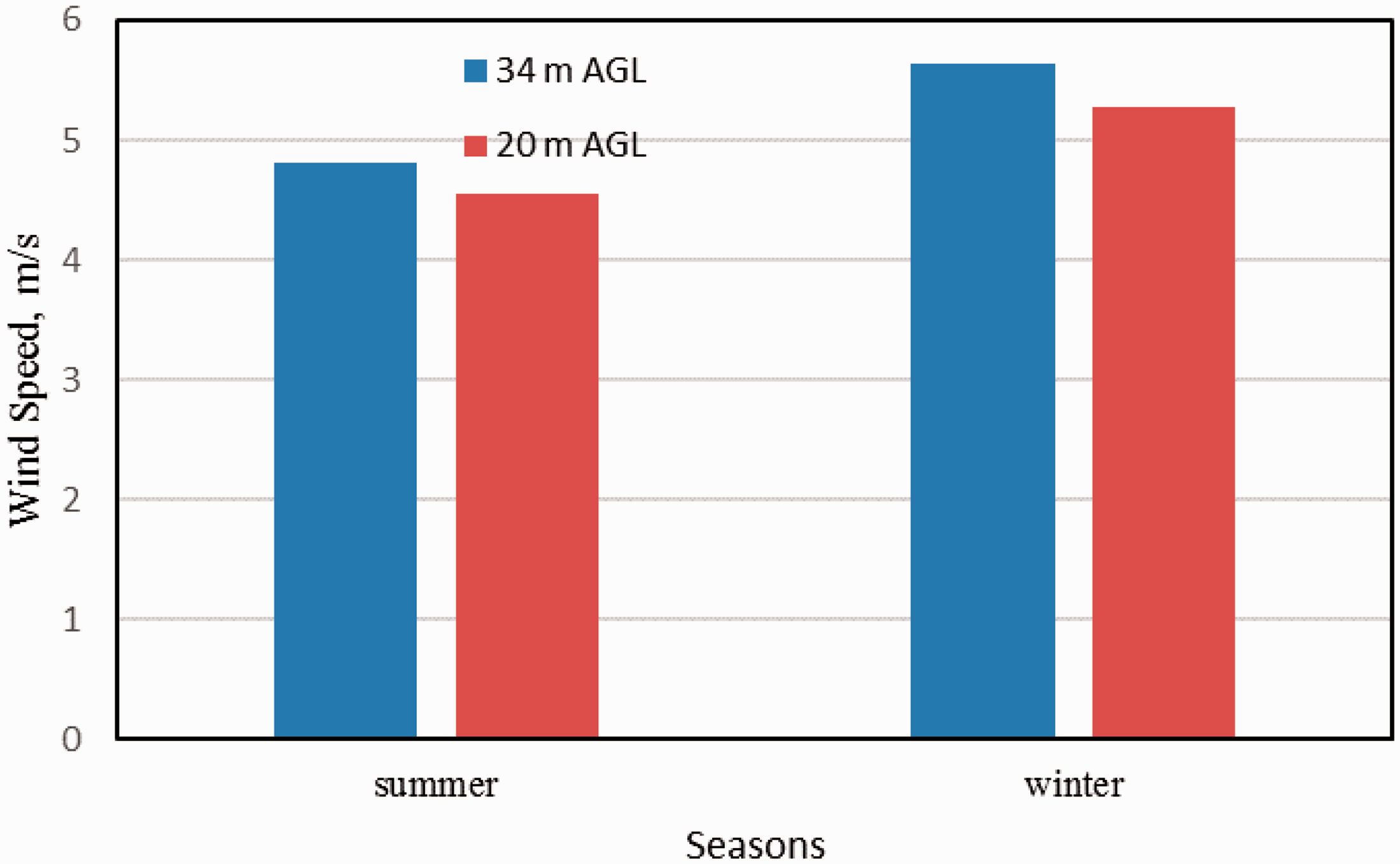
Seasonal averaged wind speeds at 34 m and 20 m AGL for the entire measurement period.

Wind shear analysis

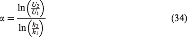
Wind shear analysis is used to express the wind profile for a site. According to Zhang (2015), “Wind profile enables us to deduce the mean wind speed from one height to another and tells us the wind speed difference between two heights.” To find the wind shear coefficient (WSC) of the site, the logarithmic formula was used as shown in equation (34).

$$\alpha =\frac{\text{ln}\left(\frac{U_2}{U_1}\right)}{\text{ln}\left(\frac{h_2}{h_1}\right)}$$

(34)

where α is the WSC, and U and h are the wind speed and the height, respectively. The basic reason of placing two anemometers at different heights is that the WSC can be estimated accurately. According to Fırtın et al. (2011), the WSC will never be constant and is similar to the wind profile but it varies with the mean wind speed, the direction of the wind flow, atmospheric condition, the time of the day, the nature of the terrain, humidity, pressure, and temperature.

The heating and the cooling cycle of air above the ground affects the WSC. From several reported works (Aukitino et al., 2017; Fırtın et al., 2011; Gualtieri and Secci, 2011; Rehman and Al-Abbadi, 2008), it is clear that during daytime the WSC is lower, while at night the WSC is higher. Heating effect of the ground surface and the air takes place during the day which results in an upward flow of air causing a reduction in the WSC. From the sunset time, the cooling effect starts and is more pronounced during the night. This phenomenon is shown in Figure 9, which shows the WSC for the overall 24 h. Starting from morning 6 a.m., the WSC decreases till 12 noon, this indicates the heating effect of the ground and the air. From 12 noon to 6 p.m., the WSC increases slightly as the temperature drops. The cooling effect is seen after 6 p.m. where the WSC increases till morning and is maximum at 6 a.m.

Figure 9.

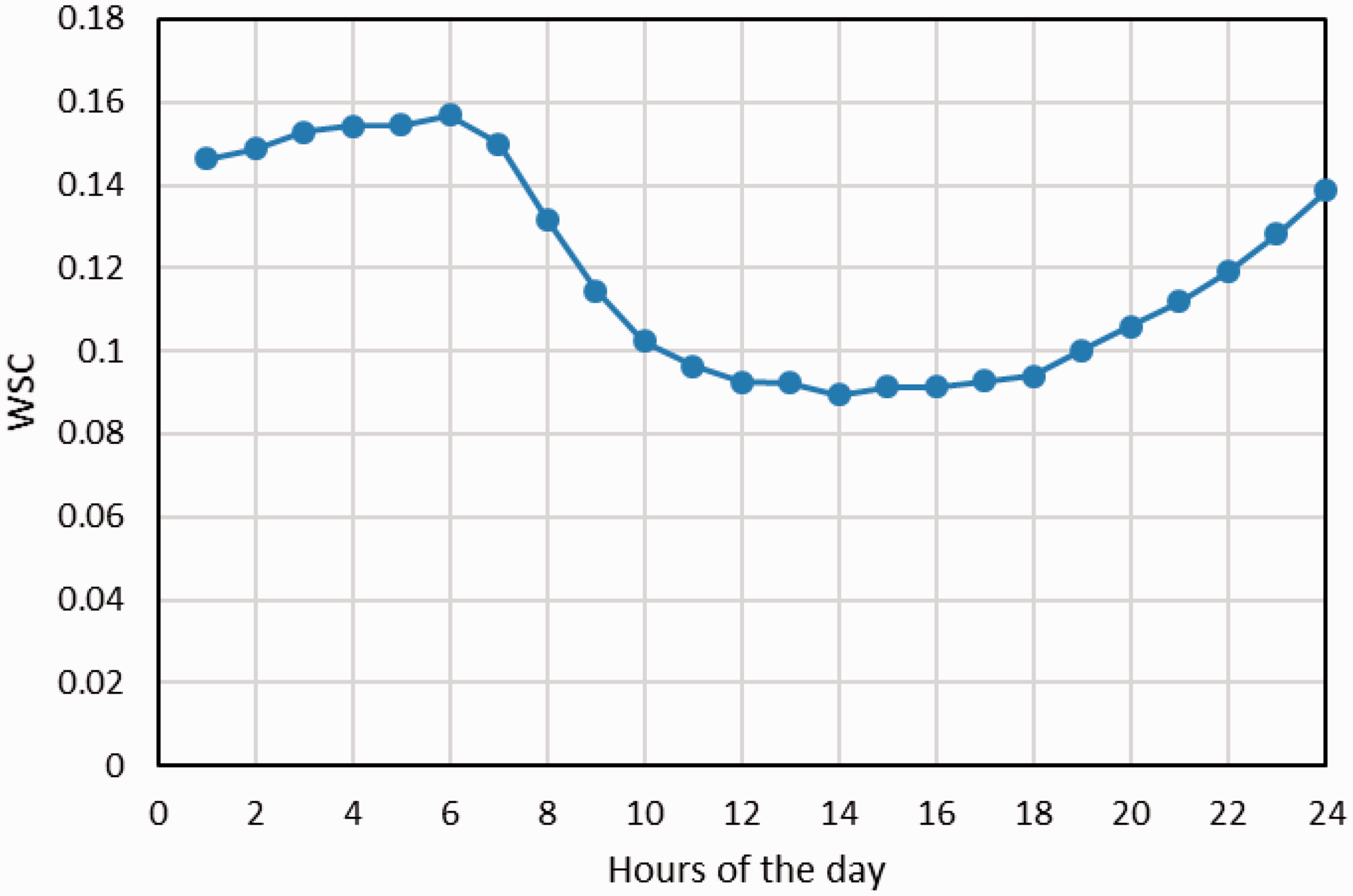
Averaged diurnal WSC, α, for the entire measurement duration.

Diurnal variation in the temperature was estimated and compared with the WSC. Figure 10 shows the diurnal variation of the temperature for the site. It was observed that the graph matches the relation of the heating and the cooling cycle. As the temperature increases, the WSC decreases, and as the temperature decreases, the WSC increases.

Figure 10.

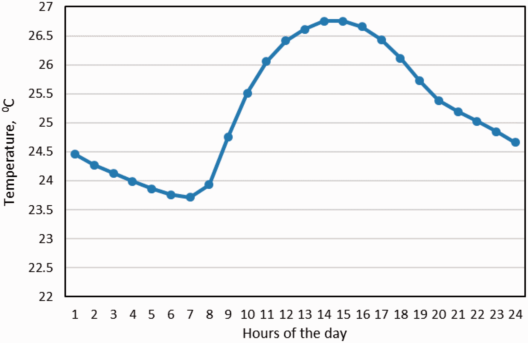
Averaged diurnal temperature variation for the entire measurement duration.

The monthly variation of the WSC was also obtained and is shown in Figure 11; it can be seen that it does not have any clear trend. From the figure, it can be seen that September has the largest WSC of 0.23, while November has the lowest WSC of 0.08.

Figure 11.

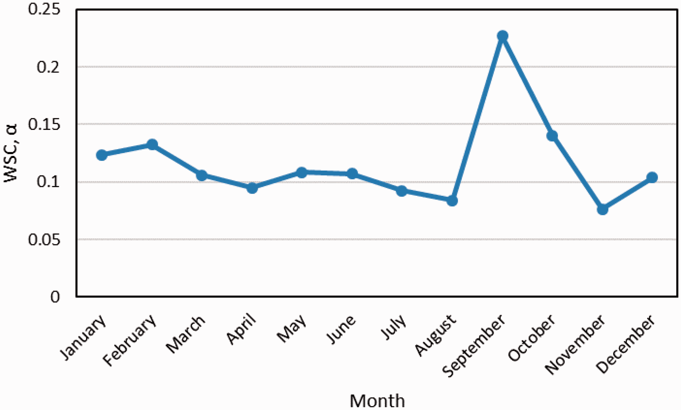
Monthly averaged WSC, α.

TI

It is well-known that for the wind turbine components, higher turbulence levels have harmful effects. Turbulence generates fatigue loads on the major component of the wind turbines. How much the wind varies is quantified with the TI. Turbulence is also known as the fluctuations in wind speed with respect to time (Aukitino et al., 2017). Using equation (35), the TI can be determined.

$$\text{TI}=\frac{{\sigma }_u}{\overline{U}}$$

(35)

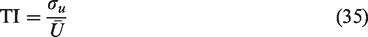
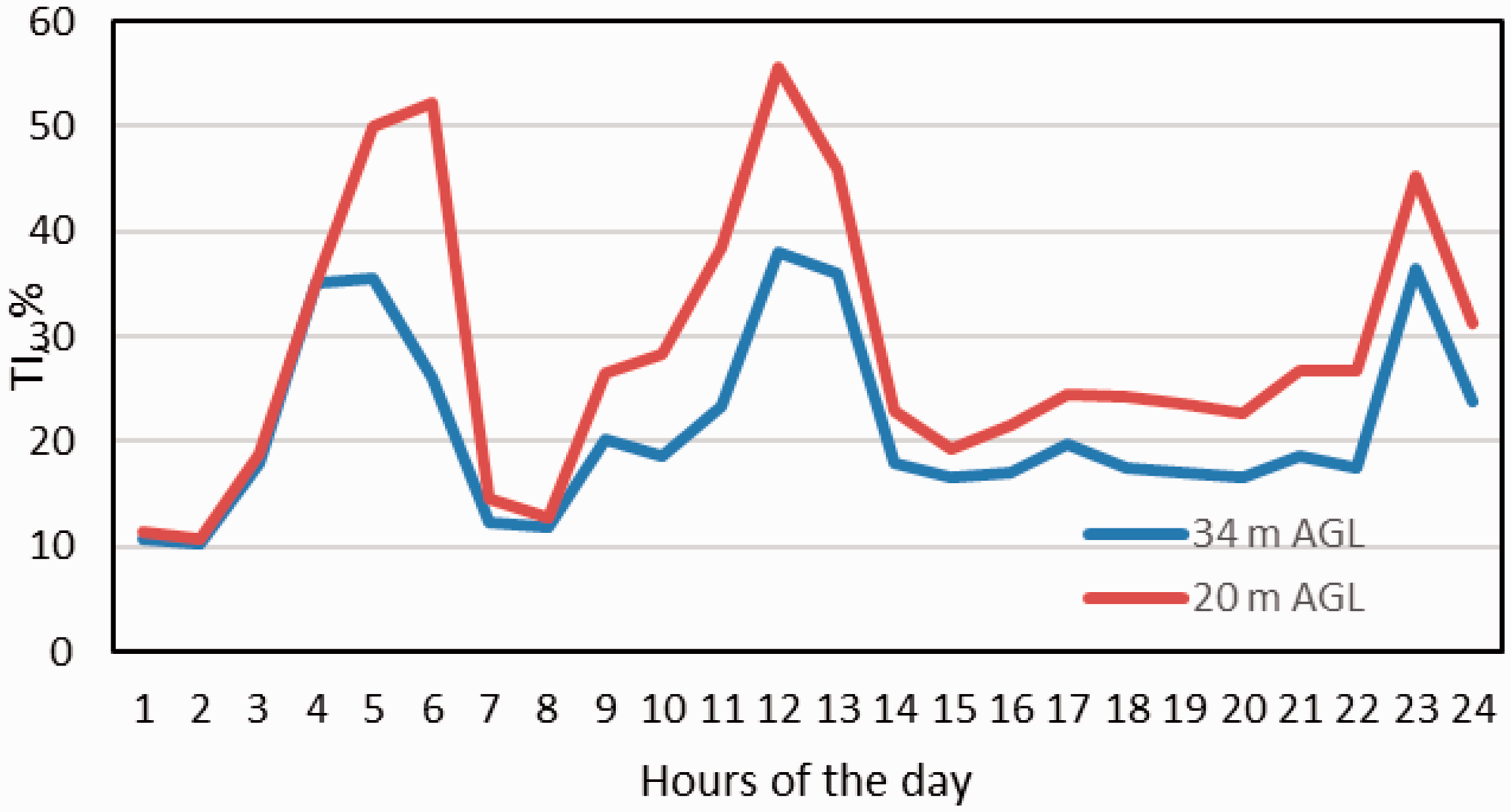
Figure 12 shows the overall TI for the entire period of study. It can be seen that the TI at 34 m AGL is less compared to that at 20 m AGL. The TI tends to be lower at greater heights as the wind flow becomes smoother due to lesser disturbances and also due to higher mean wind speed. The overall averaged TIs for the Suva site are 12.5% and 13.72% for the 34 m and 20 m AGL, respectively. It is clear from a comparison of Figures 4 and 12 that, at the time of higher wind speed, the TI is lower. From the results, it can be said that the overall averaged TI is within the range of the allowable TI of 16% for 15 m/s wind speed which suits the design standards for turbines as per IEC61400-1 standards (IEC).

Figure 12.

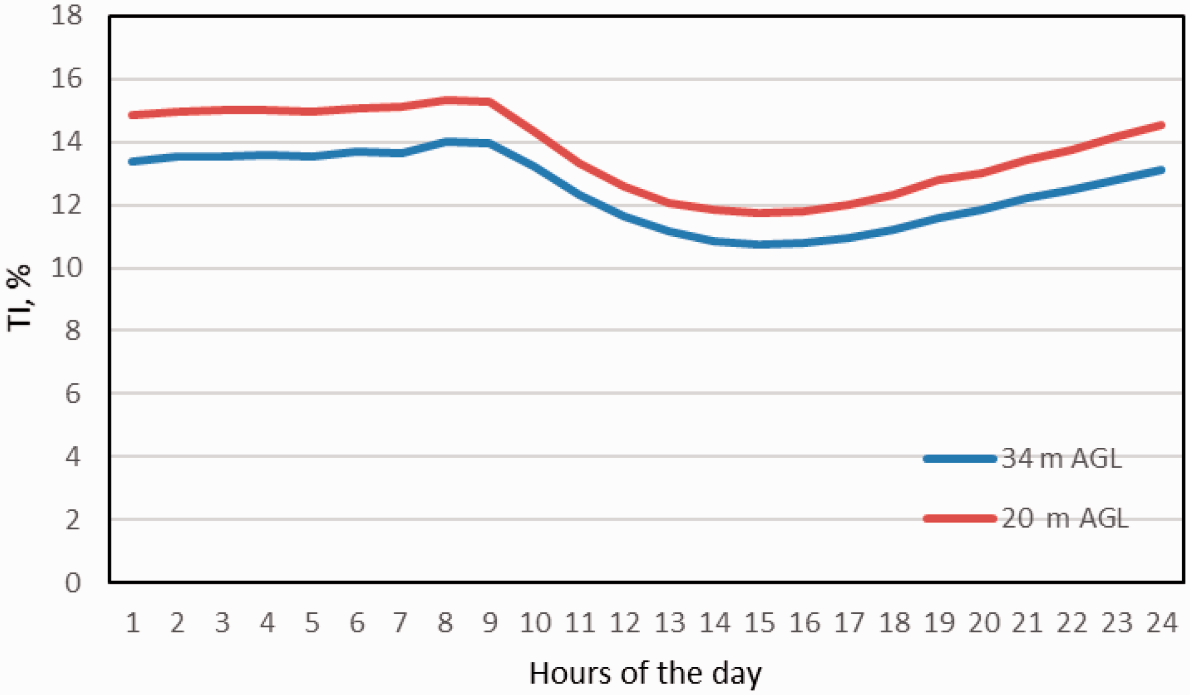
TI for the overall period.

The TI intensity for a typical windy day of June 2015 was estimated and the diurnal variation was plotted. The average wind speed for that day was 12.56 m/s and the mean TIs for this day were 9.05% and 9.75% at 34 m AGL and at 20 m AGL, respectively, as shown in Figure 13. The TI for this windy day is much lower due to higher wind speed. In the month of May in 2016, there was a low wind day where the wind speed for the day averaged 3 m/s. The mean TIs for that typical day were 21.46% and 28.71% at 34 m AGL and at 20 m AGL, respectively. When the wind speed dropped below 1 m/s, the turbulence level became very high at the time of sunrise and midday. The TIs for the low wind day are shown in Figure 14.

Figure 13.

TI for a windy day.

Figure 14.

TI for a low wind day.

WPD and direction analysis

In a wind resource assessment, the analysis of the wind direction with the available WPD is very important. In previous studies, the wind rose plots have been very common but from a recent study by Zheng et al. (2016), the WPD rose plots are found to be more useful than the wind speed rose plots. From this analysis, it can be found from which direction the maximum amount of wind power can be generated. The analysis was carried out with the wind vane placed at 30 m AGL and the anemometer placed at 34 m AGL. The WPD rose plot was divided into segments of 30°. As mentioned earlier, the data analyzed were obtained at 10 min interval and the wind direction was considered not to vary with height within the height of interest. According to Capps and Zender (2010), between the cut-in and the cut-out speeds, wind power is harvested which means that the effective wind which can be used to generate power is between these two values. The analysis is based on the cut-in and cut-off speeds of the Vergnet 275 kW wind turbine which will be used for estimating the AEP and for performing an economic analysis in later section. The cut-in speed of the Vergnet 275 kW wind turbine is 3 m/s, while the cut-off speed is 25 m/s. The effective wind, which is between 3 m/s and 25 m/s, recorded for the overall 10 min wind measured data is 74.175% of the time. It is seen that the effective wind shown via the WPD is more for winter than summer, and the effective percentage WPD recorded for summer and winter was 69.74% and 79.47%, respectively. Figure 15 shows the overall effective wind energy rose plot based on the cut-in and cut-out wind speeds for the overall period for the Suva site. The predominant wind direction for the site was between 60° and 150°. There was no major difference in the summer- and winter-averaged wind direction as can be seen from Figures 16 and 17, respectively. The predominant wind directions for these seasons were also between 60° and 150°. Overall, the maximum energy will be harnessed from the eastward direction. Fiji has the dominant wind force of southeast trade winds, but due to the site location (terrains), the prevalent wind is mostly eastwards. The site being very close to the sea, sea-breeze and land-breeze also play an important role. Figure 18 shows the hourly averaged effective WPD. The hourly averaged WPD ranged mostly between 50 W/m² and 100 W/m² but some averages were higher. The hourly averaged maximum WPD is 362 W/m² at the wind speed of 25 m/s.

Figure 15.

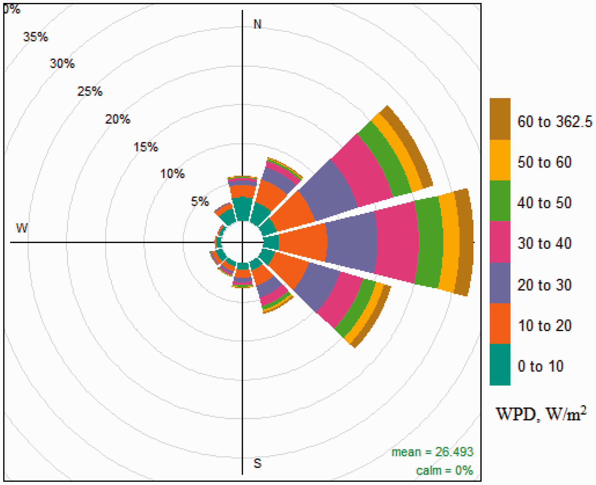
WPD rose plot for the overall period.

Figure 16.

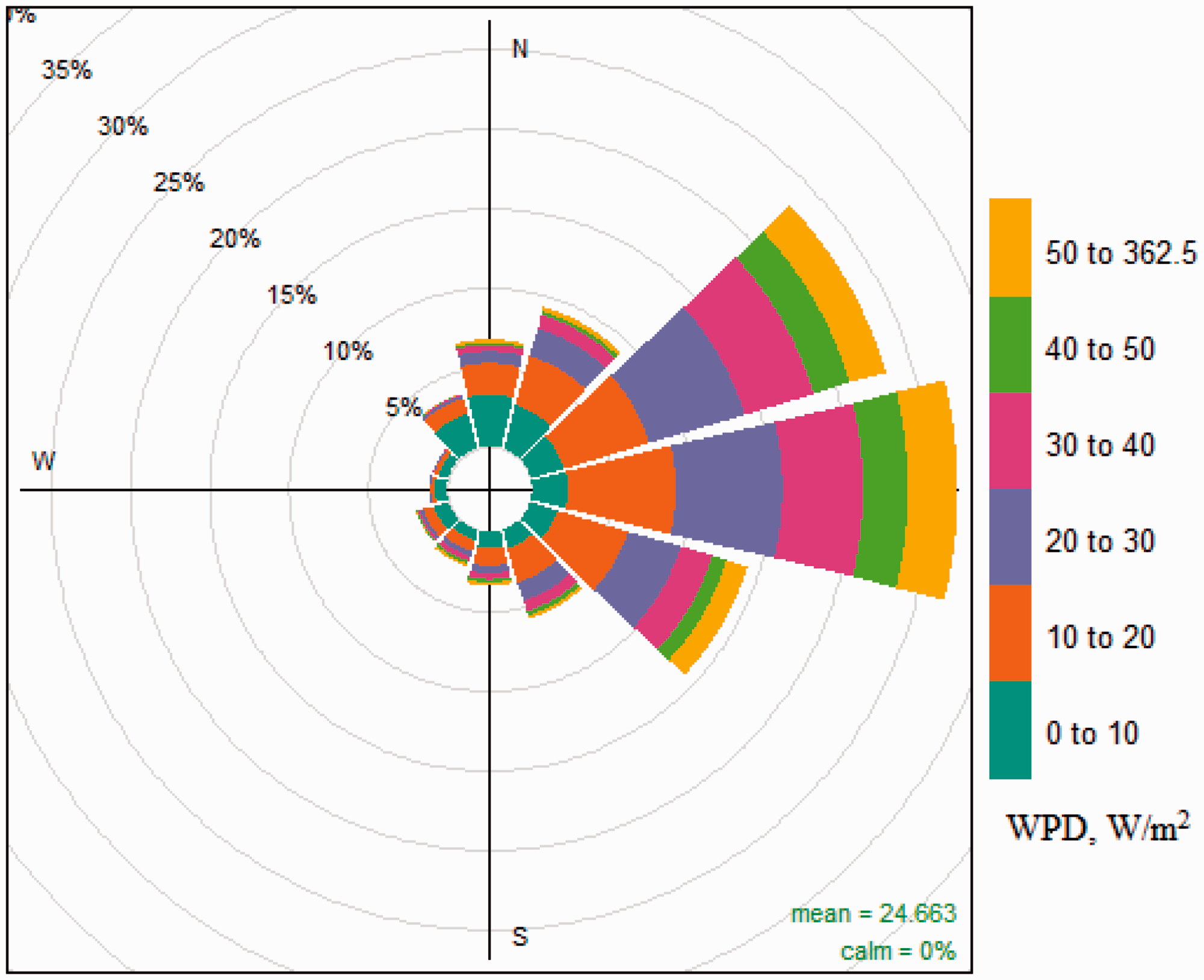
WPD rose plot for summer.

Figure 17.

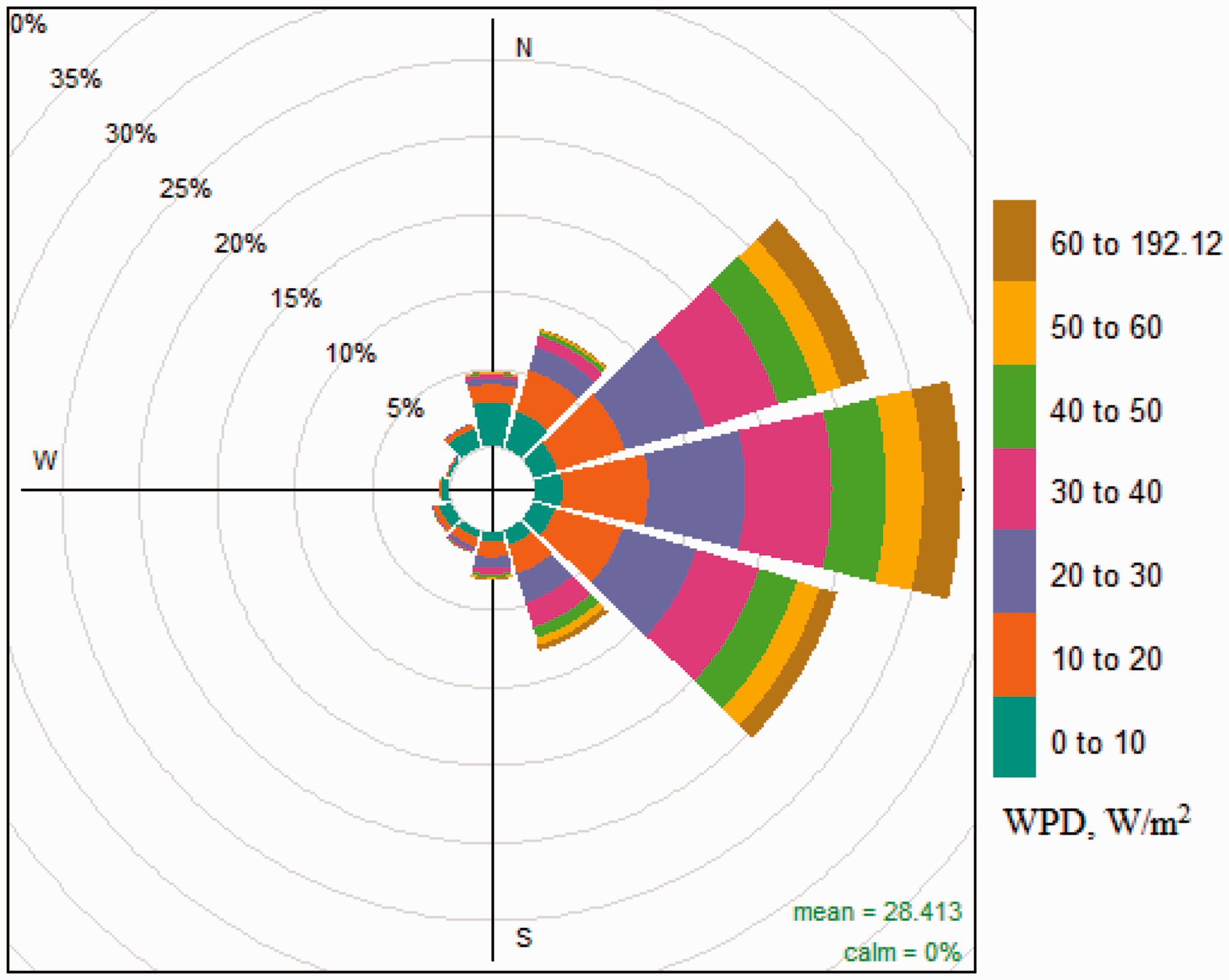
WPD rose plot for winter.

Figure 18.

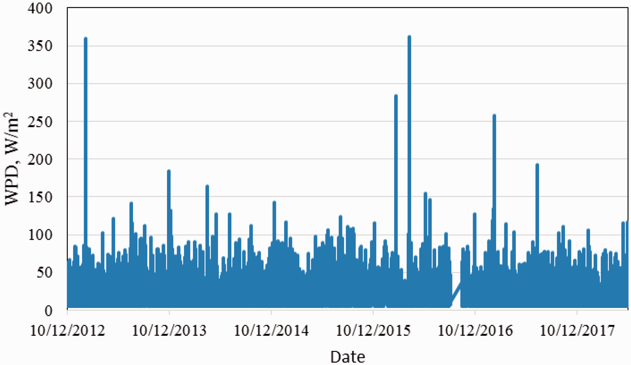
Hourly averaged effective WPD for the duration of measurements.

Weibull parameters and their accuracy

The Weibull parameters for the entire period of study were estimated using the 10 different methods and are shown in Table 2. Based on the best fit obtained with the help of error estimation, the best method was selected. From the results, it can be seen that the best method is the EMJ. This method is the best method because in the error analysis it has overall lowest ranking as seen in Table 3. While it gives the fourth highest R² value, it gives the second lowest RMSE and MAE values, and third lowest COE value, giving it the best rank overall. While MM gave the highest R² value, the other error parameters were way behind other methods. The other method that showed lowest error estimations was the MO with the lowest RMSE and MAE values, but the other error parameters were considerably behind those of other method, ultimately giving it an overall second rank.

Table 2.

Methods of estimating Weibull parameters, the k and A values, mean wind speed and WPD, and goodness of fit test/errors.

Method	k	A	U	WPD	R 2	COE	RMSE	MAE	MAPE
MQ	1.73	6.43	5.730613	244.6804	0.9834	0.8356	0.5696	0.3651	8.0592
MO	1.93	5.85	5.188653	160.5405	0.9851	1.0617	0.3602	0.2791	8.117
EMJ	1.94	5.85	5.187931	159.4656	0.9853	1.0708	0.3614	0.2812	8.3008
EML	1.94	5.85	5.187931	159.762	0.9853	1.0697	0.3619	0.282	8.3258
LS	1.64	5.62	5.02794	177.709	0.9747	0.8974	0.5118	0.4073	8.5859
ML	1.87	5.82	5.167275	164.2095	0.9834	1.0248	0.3707	0.2814	7.511
MML	1.83	5.76	5.118416	162.783	0.9826	1.0118	0.3868	0.2946	7.123
EPF	1.98	5.85	5.185445	156.1209	0.9858	1.1013	0.3713	0.2906	8.962
WASP	2.23	6.1	5.402637	157.9151	0.9864	1.2229	0.498	0.3382	12.9398
MM	2.16	6.73	5.960115	217.6643	0.9884	1.0581	0.7733	0.7181	19.953

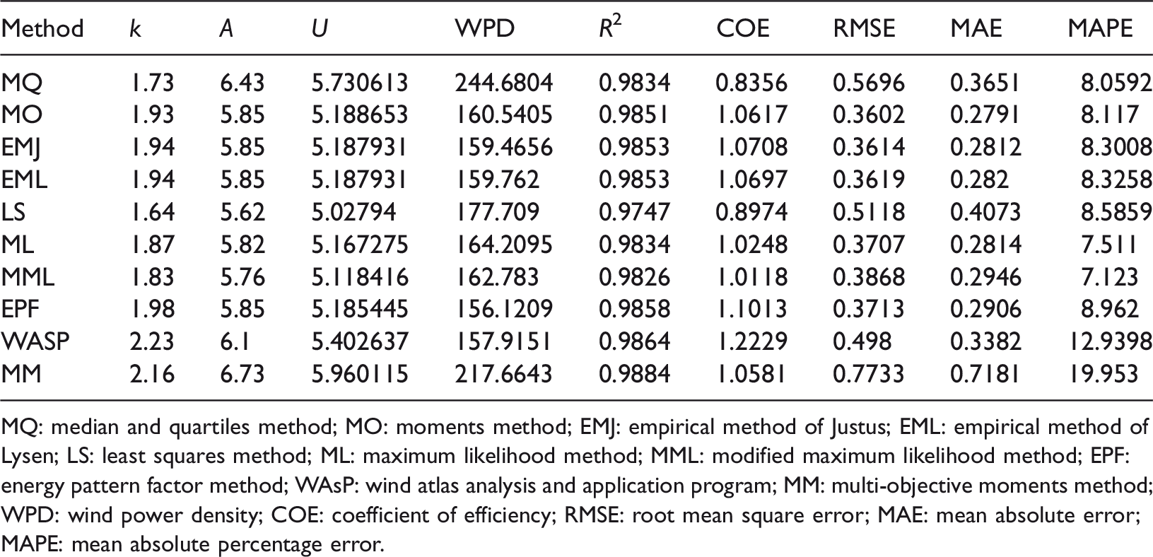
MQ: median and quartiles method; MO: moments method; EMJ: empirical method of Justus; EML: empirical method of Lysen; LS: least squares method; ML: maximum likelihood method; MML: modified maximum likelihood method; EPF: energy pattern factor method; WAsP: wind atlas analysis and application program; MM: multi-objective moments method; WPD: wind power density; COE: coefficient of efficiency; RMSE: root mean square error; MAE: mean absolute error; MAPE: mean absolute percentage error.

Table 3.

Performance evaluation by ranking.

Method	k	A	U	WPD	R 2	COE	RMSE	MAE	MAPE	RANK
EMJ	1.94	5.85	5.187931	159.4656	4	3	2	2	5	1
MO	1.93	5.85	5.188653	160.5405	6	5	1	1	4	2
EML	1.94	5.85	5.187931	159.762	5	4	3	4	6	3
EPF	1.98	5.85	5.185445	156.1209	2	2	5	5	8	4
ML	1.87	5.82	5.167275	164.2095	8	7	4	3	2	5
MML	1.83	5.76	5.118416	162.783	9	8	6	6	1	6
WASP	2.31	6.3	5.581549	169.0733	3	1	9	9	9	7
MQ	1.73	6.43	5.730613	244.6804	7	10	8	7	3	8
MM	2.16	6.73	5.960115	217.6643	1	6	10	10	10	9
LS	1.64	5.62	5.02794	177.709	10	9	7	8	7	10

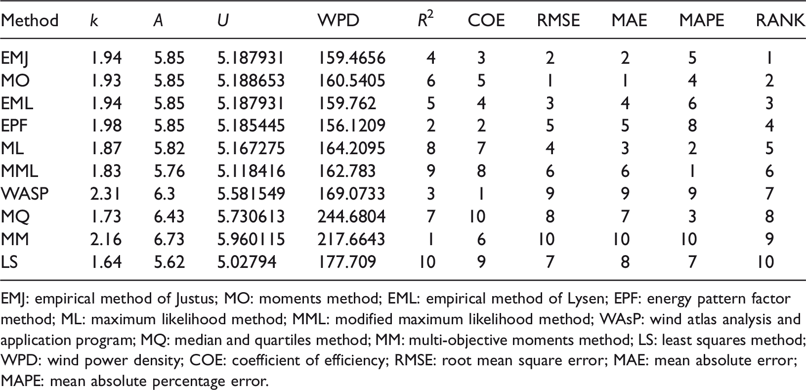
EMJ: empirical method of Justus; MO: moments method; EML: empirical method of Lysen; EPF: energy pattern factor method; ML: maximum likelihood method; MML: modified maximum likelihood method; WAsP: wind atlas analysis and application program; MQ: median and quartiles method; MM: multi-objective moments method; LS: least squares method; WPD: wind power density; COE: coefficient of efficiency; RMSE: root mean square error; MAE: mean absolute error; MAPE: mean absolute percentage error.

Table 4.

AEP from five Vergnet 275 kW turbines in the Suva city.

Turbine site	Location (m)	Geographic location	Power density (W/m2)	Net AEP (MWh)	Capacity factor (%)
1	(652,000, −2,008,900)	18° 9′ 49.96″S	164	426.69	17.7
		178° 26′ 9.92″E
2	(654,000, −2,007,200)	18° 8′ 53.80″S	160	417.603	17.3
		178° 27′ 20.92″E
3	(651,340, −2,004,000)	18° 7′ 10.39″S	127	327.713	13.6
		178° 25′ 49.57″E
4	(650,600, −2,007,000)	18° 8′ 48.21″S	151	391.802	16.2
		178° 25′ 18.38″E
5	(656,300, −2,004,000)	18° 7′ 9.11″S	148	385.653	16
		178° 28′ 38.30″E

Seasonal Weibull parameters

The Weibull parameters for the two different seasons were found by the same analysis as done for finding the Weibull parameters for the entire period. The dataset was first divided into the two seasons’ datasets for the dry season (winter) and wet season (summer). For the summer season, the MO was found to be the best method but for winter the best method was found to be the EMJ.

Wind speed frequency distribution

The overall wind speed data were divided into bins of wind speeds. Based on different Weibull parameter estimation methods, the Weibull curves for the 10 different methods were drawn and are shown in Figures 19–21. From the graphs, it is noted that wind speed was mostly between 0 m/s and 8 m/s; however, for the winter season, higher wind speeds were more frequent, as can be seen from Figure 21. The effective wind for the site is between 5 m/s and 8 m/s throughout.

Figure 19.

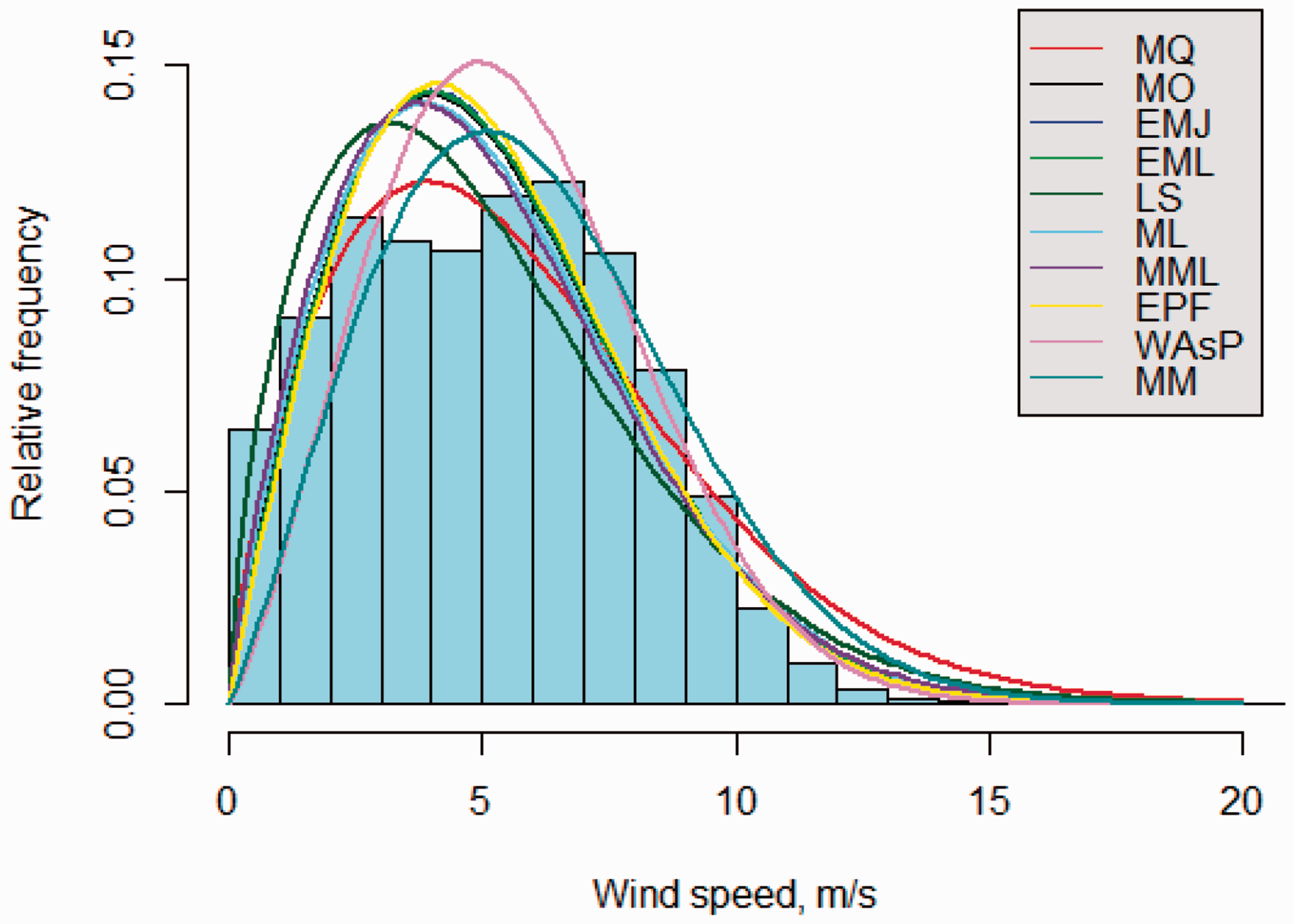
Wind frequency distribution and Weibull curves from 10 different methods for the overall period.

Figure 20.

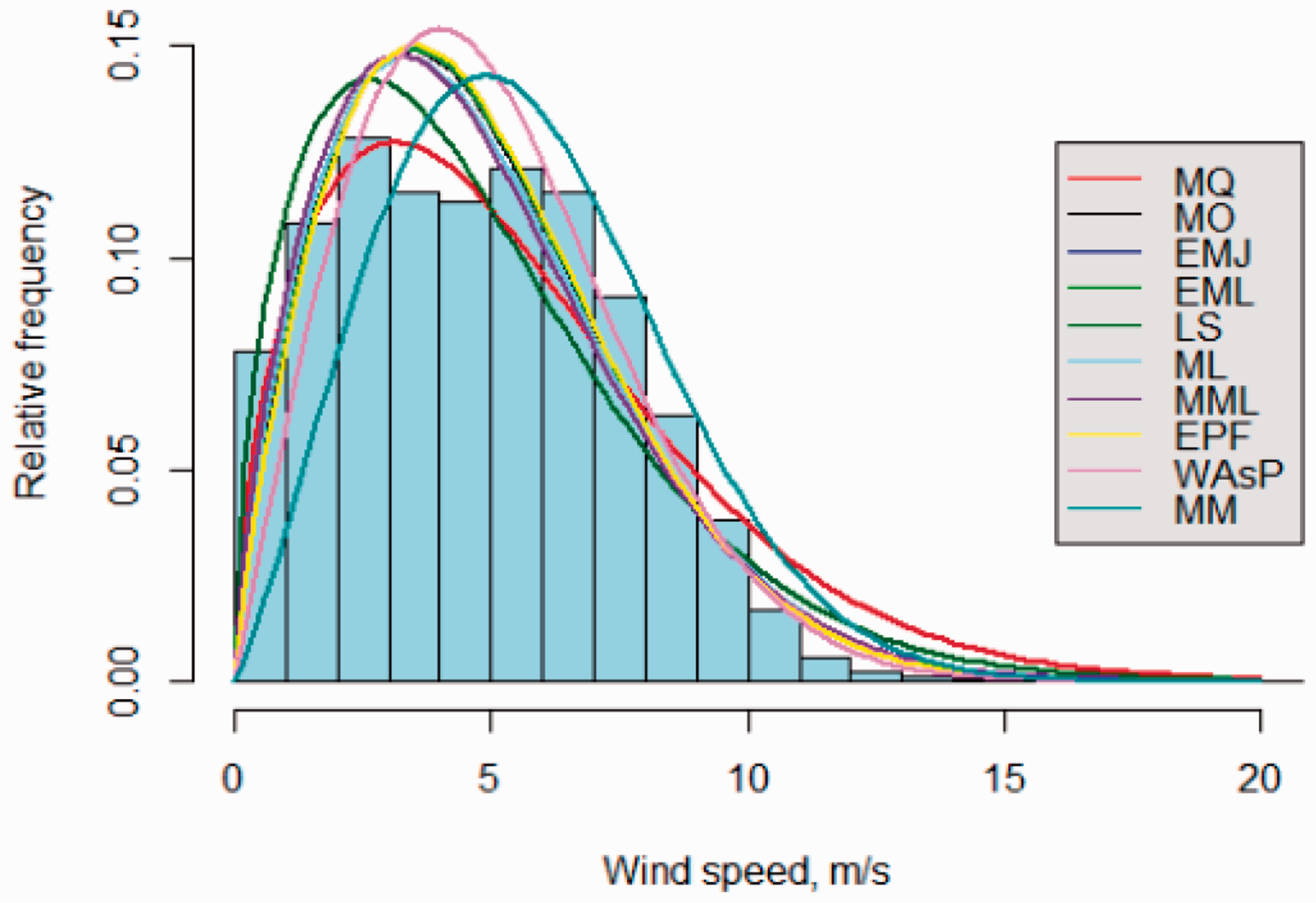
Wind frequency distribution and Weibull curves from 10 different methods for summer.

Figure 21.

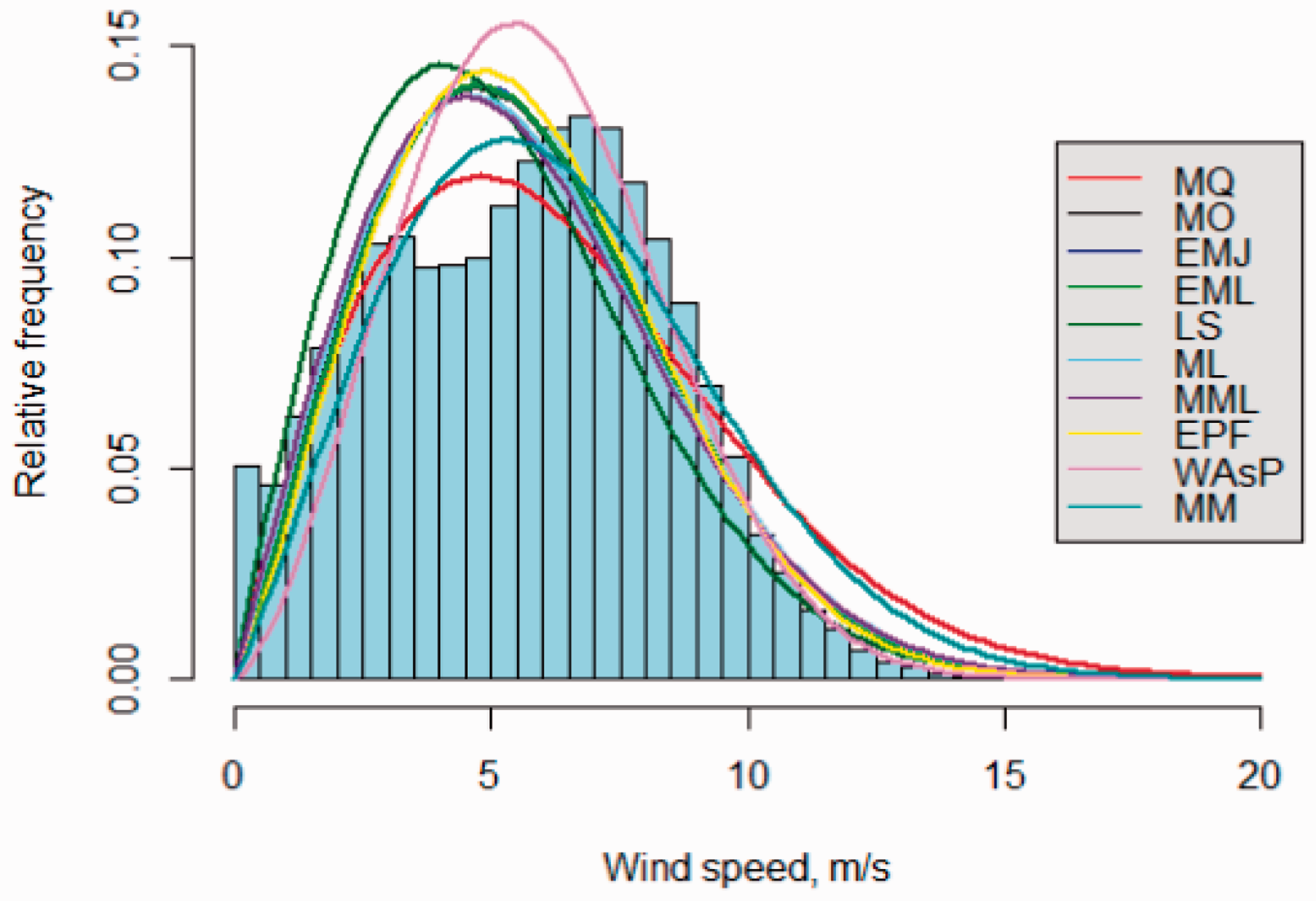
Wind frequency distribution and Weibull curves from 10 different methods for winter.

Resource grid

The resource grid of the WPD of the site was drawn using the WAsP software. The resource map is drawn on the basis of the resolution of the map which is the rectangular sets of points on the map. With the help of resource maps, we can manage the set of points for which a summary of wind predicted climate data is calculated. The points are arranged into rows and columns and are regularly spaced. Each point in the grid is the simpler version of a normal turbine site. To develop a resource map, the resource grid must be associated with a generalized wind climate and needs to be entirely located in the associated map. For realistic modeling of every point in the grid, there should be at least 5–10 km of terrain from any point in the grid to any border of the map. For each point in the resource map, WAsP calculates the elevation, mean wind speed, and mean power density along with other parameters. To obtain the resource grid, first the generalized wind climate is calculated. The next step is to digitize the vector map. To digitize the map, the terrains and roughness levels need to be defined. For the area, the WAsP calculates the WPD, wind speed, Weibull parameters as well as some other parameters. The resource map of WPD for Suva based on the digitized map is shown in Figure 22. The maximum WPD is found at the peak of the terrains/mountains. Suva city is built on terrains not like some other cities where the land is more or less level. Suva has most of its land covered with buildings as well as trees. The WPD for most of the area covered is between 120 W/m² and 200 W/m² and the peak is having a WPD of 337 W/m².

Figure 22.

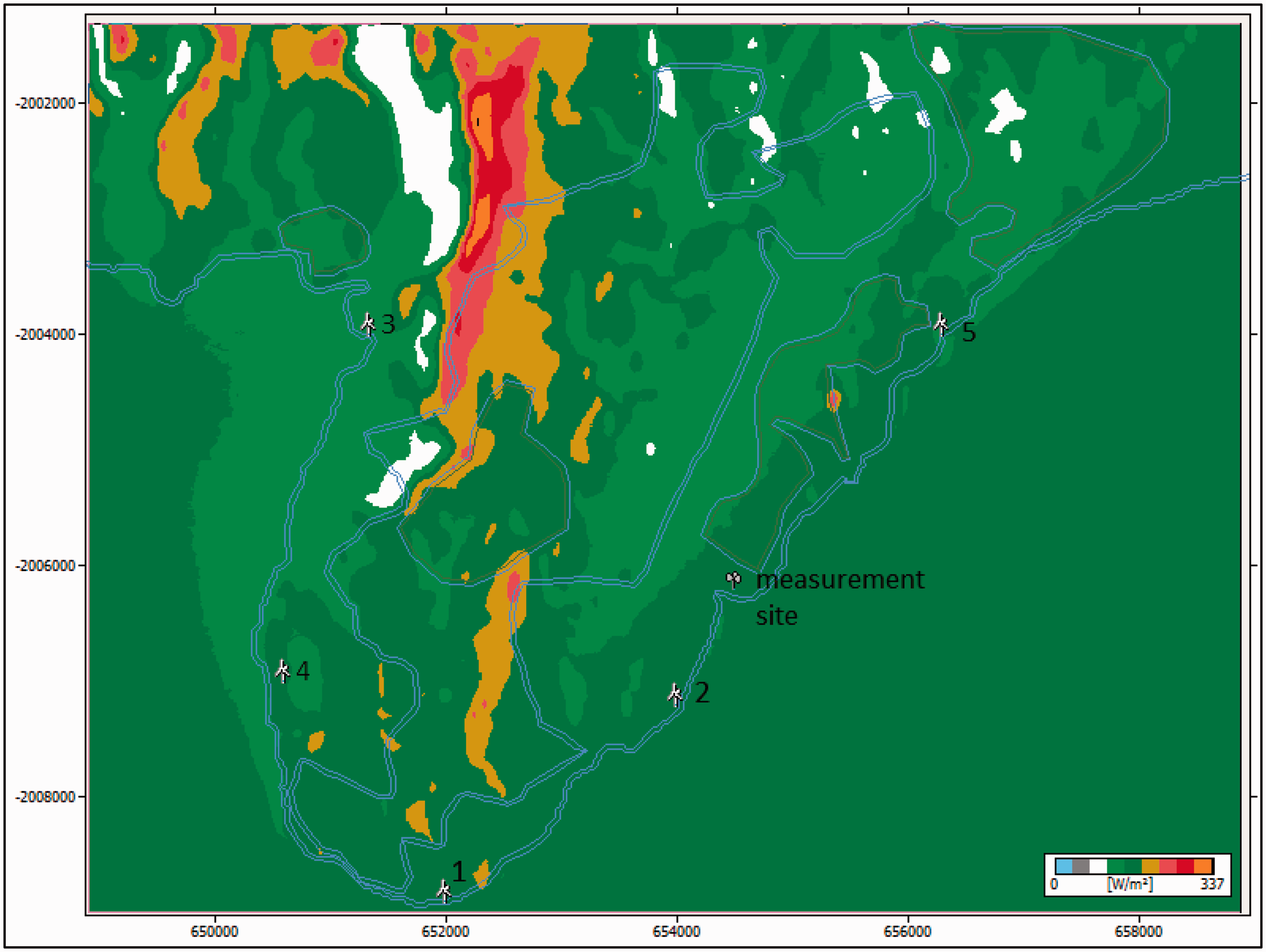
High-resolution overall WPD map of Suva city. The numbers 1–5 indicate the location of preferred installation sites for the turbines.

For explicit analysis, there were five sites selected for installation of the wind turbines. The sites chosen are close to the shoreline and have effective WPD potential based on the high-resolution resource grid map which is shown in Figure 22. The AEP was calculated for each selected site which is shown in the next section to show how much energy can be harvested if we place a turbine at the selected location and also since Suva is not very highly populated; however, it is one of the most populated cities in the South Pacific region, placing a large wind farm will not be possible due to non-availability of large land; thus, scattering the turbines and locating them at sites of high wind speeds will be a good solution.

AEP

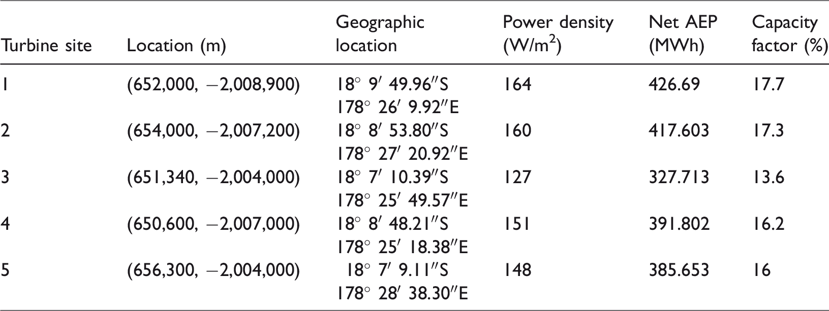
Using the Vergnet 275 kW wind turbine, the AEP was estimated using WAsP, as shown in Table 4. WAsP has become one of the main tools in wind industry for estimations of AEP for small wind turbines as well as for large-scale wind farms. For estimation, the hub height of the turbine was taken as 34 m, a rotor diameter of 32 m, a cut-in speed of 3 m/s, rated wind speed of 12.2 m/s with a density of 1.16 kg/m³, and a cut-out wind speed of 25 m/s. The power curve of the turbine is shown in Figure 23.

Figure 23.

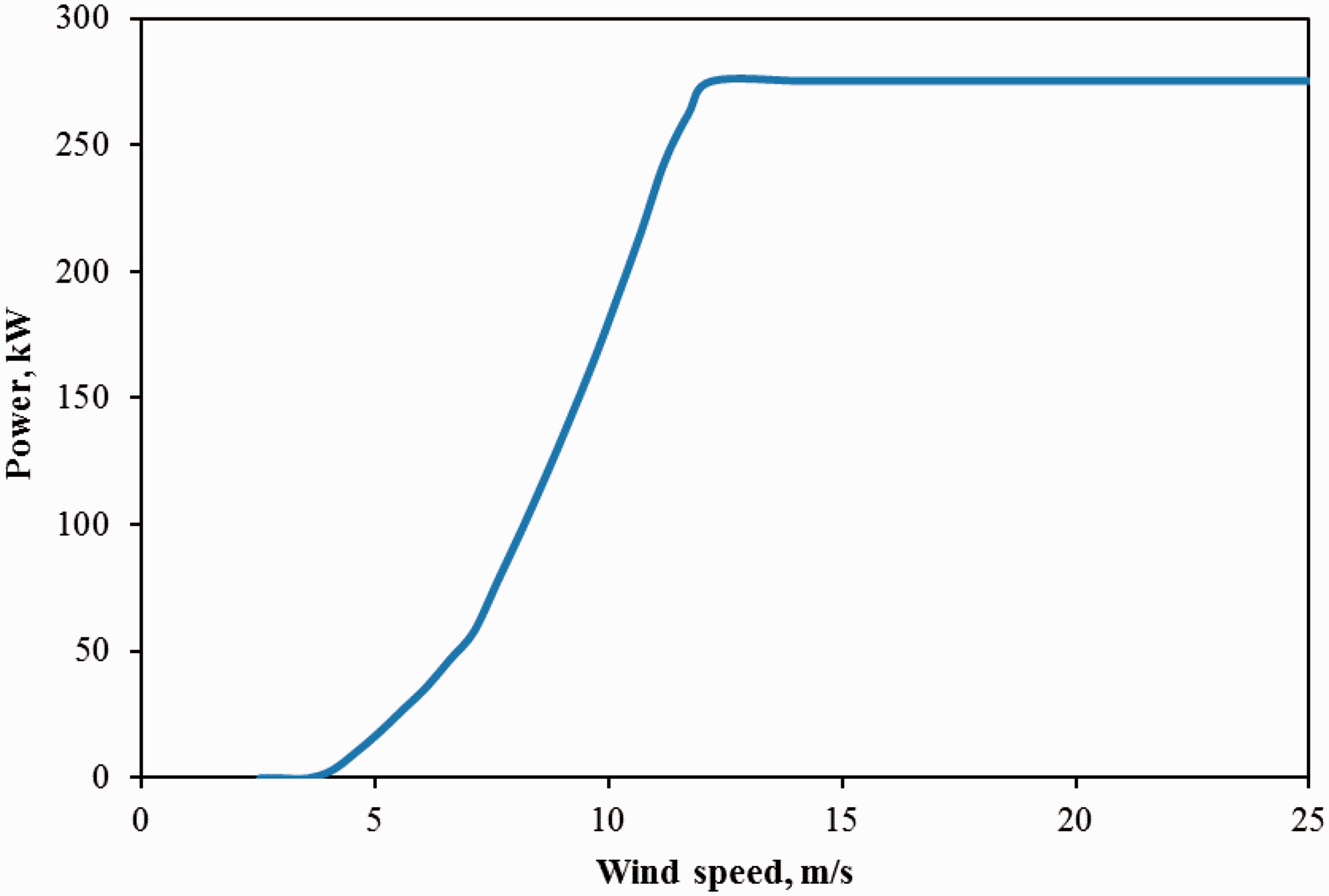
Power curve for the Vergnet 275 kW wind turbine.

The Vergnet turbines are chosen for many reasons: the turbines are easier to lower during cyclones, easier to maintain, and also these turbines have already been installed and are performing very well in Vanuatu as well as in Fiji. A number of other turbines could be used so that the AEP could be increased but due to higher initial costs, these turbines are excluded. The other problem is noise—if large turbines are installed, there would be high noise levels and this will become another major concern for the dense population of Suva. The AEP for all the five turbines was estimated using WAsP.

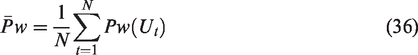
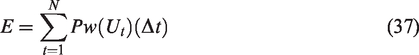
The average power generated by a turbine is obtained by taking the averaged wind speed for the time interval from time $t_i$ to $t_i+\Delta t$ for the period of N observations expressed through

$$\overline{P}w=\frac{1}{N}{\displaystyle \sum _{t=1}^N\mathit{Pw}(U_t)}$$

(36)

where $\mathit{Pw}(U_t)$ is the power output defined by the turbine power curve. The energy yield from the turbine can be expressed as:

$$E={\displaystyle \sum _{t=1}^N\mathit{Pw}(U_t)}(\Delta t)$$

(37)

For the analysis, the Vergnet 275 kW two-bladed wind turbines are chosen for all sites’ power output estimation. The sites selected for the turbines are close to shorelines and are flat surfaces and for all the turbines, hub heights are selected to be 34 m AGL. The error in the estimation of wind speed will be negligible, since the measurements are performed at a height of 34 m AGL. The total AEP for all the five selected sites is 2029 MW for one year. The average capacity factor for the all five sites together is 17%. The capacity factor is the generated AEP over the expected AEP for the wind farm. The wake loss for all the turbines is 0%. The AEP for the five turbine sites ranged from 344 MW to 442 MW. The power density also was high ranging from 127 W/m² to 164 W/m².

Economic analysis

The economic analysis of installing five Vergnet turbines at the above sites was carried out. For the analysis, the following assumptions were taken into account:

All amounts are in US$.

The lifetime (T) of the turbine is assumed to be 20 years.

The interest rate (r) and inflation rate (i) are considered to be 12% and 3%, respectively.

Operational maintenance/repair costs (C_omr) are considered to be 25% of the annual cost of the turbine (machine price/lifetime).

Scrap value (S) is taken as 10% of the cost of the turbine and civil work.

Investment (I) includes the cost of the turbine plus its transportation cost to Fiji and the cost of the civil work and the costs associated with grid integration.

For calculating the present value of cost is expressed by the following equation:

$$\text{PVC}=I+C_{\text{omr}}\left[\frac{1+i}{r-i}\right]\left[1-{\left(\frac{1+i}{1+r}\right)}^T\right]-S{\left(\frac{1+i}{1+r}\right)}^T$$

(38)

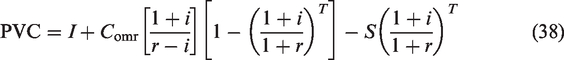
The cost of a Vergnet 275 kW wind turbine for Fiji is US$615,000 (including US$35,000 transport cost to Fiji). The operation maintenance and repair cost (C_omr) is equal to US$615,000/20 × 0.25 comes to US$7,687.50. The scrap value, S, comes to US$58,000. The scrap value is the 10% of the initial cost. The interest rate and inflation constants are taken as 0.12 and 0.03, respectively. Thus, the present value cost using equation (38) comes to US$675,647.

The total AEP for the five turbines is 1950 MWh. The period for maintenance is neglected. The EFL sells electricity to its consumers at FJ$0.33/kWh (charge/unit) which is US$0.16/kWh. The average cost of each kWh energy produced by a turbine will be equal to US$675,647/(20 × 390 MWh) which is US$0.09/kWh. The amount recovered for one turbine per year would be US$62,400 based on the current price of electricity in the country (US$0.16). To recover the full expense on one generator based on the current rate, it will take 10.83 years. If this type of wind turbine with the combination of other energy sources which are solar and hydro is used, the cost of electricity could be reduced, making the country pollution free.

Conclusion

There is a reasonably good wind energy potential in Suva, Fiji. Wind resource assessment for Suva is carried out after a long measurement campaign of more than five years. The data analysis shows that the overall average wind speed for the site is 5.18 m/s at 34 m AGL. The seasonal mean wind speeds were not alike; the winter month showed higher wind speeds compared to the summer months. The wind speed for summer was 4.8 m/s, and 5.64 m/s for winter. This is due to the reason that Suva falls under the rainforest climate where there are no true dry seasons. The wind shear analysis was done and it was observed that the heating and cooling effects are observed. The wind from the eastwards has the most effective wind which is used for power generation. The wind data analyzed shows that 74.175% produced is the most effective wind for power generation. The TI was found for the overall as well as for the windy and low wind days. It was observed that the overall average TI was 12.5% and 13.72% for the 34 m and 20 m, respectively. The TI for the windy day was lower compared to a low wind day which had a very high TI. The Weibull parameter analysis was done and it was found that EMJ was the best Weibull approximation method to find the parameters k and A. The WPD for the site based on the EMJ was 159.46 W/m². The map for the Suva city was digitized and the WPD map was drawn. An economic analysis was carried out and it was found that installing Vergnet 275 kW wind turbines will take 10.83 years to recover the cost incurred when installing the turbines.