Sage Journals: Discover world-class research

Abstract

We have studied the hydrocarbon production from oil shale reservoirs filled with diverse initial saturations of fluid phases by implementing numerical simulations of various thermal in-situ upgrading processes. We use our in-house fully functional, fully implicit, and non-isothermal simulator, which describes the in-situ upgrading processes and hydrocarbon recovery by multiphase-multicomponent systems. We have conducted two sets of simulation cases—five-spot well pattern problems and Shell In-situ Conversion Process (ICP) problems. In the five-spot well pattern problems, we have analyzed the effects of initial fluid phase that fills the single-phase reservoir and thermal processes by four cases—electrical heating in the single-phase-aqueous reservoir, electrical heating in the single-phase-gaseous reservoir, hot water injection in the single-phase-aqueous reservoir, and hot CO₂ injection in the single-phase-gaseous reservoir. In the ICP problems, we have analyzed the effects of initial saturations of fluid phases that fill two-phase-aqueous-and-gaseous reservoir by three cases—initial aqueous phase saturations of 0.16, 0.44, and 0.72. Through the simulation cases, system response and production behavior including temperature profile, kerogen fraction profile, evolution of effective porosity and absolute permeability, phase production, and product selectivity are analyzed. In the five-spot well pattern problems, it is found that the hot water injection in the aqueous phase reservoir shows the highest total hydrocarbon production, but also shows the highest water-oil-mass-ratio. Productions of phases and components show very different behavior in the cases of electrical heating in the aqueous phase reservoir and the gaseous phase reservoir. In the ICP problems, it is found that the speed of kerogen decomposition is almost identical in the cases, but the production behavior of phases and components is very different. It is found that more liquid organic phase has been produced in the case with the higher initial saturation of aqueous phase by the less production of gaseous phase.

Keywords

Oil shale kerogen in-situ upgrading electrical heating hot fluid injection In-situ Conversion Process (ICP)

Introduction

Increasing energy demand necessitates the stable energy supply by technically and economically feasible production of energy sources. Oil shales are organic-rich sedimentary rocks, where solid organic matter—kerogen—occupies the pores. Kerogen is decomposed into multicomponent materials of fluids and solids in the environments of high temperature. Fluids include a number of species including liquid and gaseous hydrocarbons. Among the unconventional resources that have been actively researched, oil shales are believed to have tremendous reserves in the United States, approximately 75% of the world’s oil shales (Knaus et al., 2010).

To heat the kerogen in oil shales to its pyrolysis temperature, a few technologies can be applied such as mining followed by surface retorting with direct/indirect heating, in-situ upgrading process, and in-situ combustion approach. Among them, the in-situ upgrading process introduces heat into kerogen while it is located in the subsurface as in its natural state. In-situ upgrading process has several advantages over surface retorting and in-situ combustion; it can be applied to deep and thick deposits with less water requirement, emissions of pollutants, and environmental impacts (Crawford and Killen, 2010). There have been plenty of studies on the diverse methods of in-situ upgrading of oil shales including Shell In-situ Conversion Process (ICP), ExxonMobil Electrofrac, EGL Technology of American Shale Oil, LLC (AMSO), and Texas A&M Steamfrac (Crawford and Killen, 2010; Symington, 2006; Thoram and Ehlig-Economides, 2011; Vinegar, 2006).

In-situ upgrading process has a few challenges as well; far longer heating time is required than surface retorting, but excess heat should be avoided because it can reduce oil quality and energy efficiency and cause environmental impacts; shale is not a good conductor of heat, and natural or induced fracture systems are necessary to distribute the heat effectively (Crawford and Killen, 2010); and the cost of in-situ upgrading is estimated to be high by significant operating cost in the case of hot fluid injection process and significant fixed cost in the case of electrical heating, respectively (Lee, 2014). In this regard, Shell ICP is an effective method to evenly heat the oil shales using densely located multiple heaters in hexagonal patterns. Shell has been developing oil shale technologies for more than 50 years including experiments and field production test and produced over 1000 bbls of oil by applying ICP in the Mahogany Demonstration Project-South (MDP-S) (Fowler and Vinegar, 2009). The delineation of general ICP method is shown in Figure 1. Converted fluids by the conductive heating process from the hexagonally installed heaters are produced at the producing wells.

Figure 1.

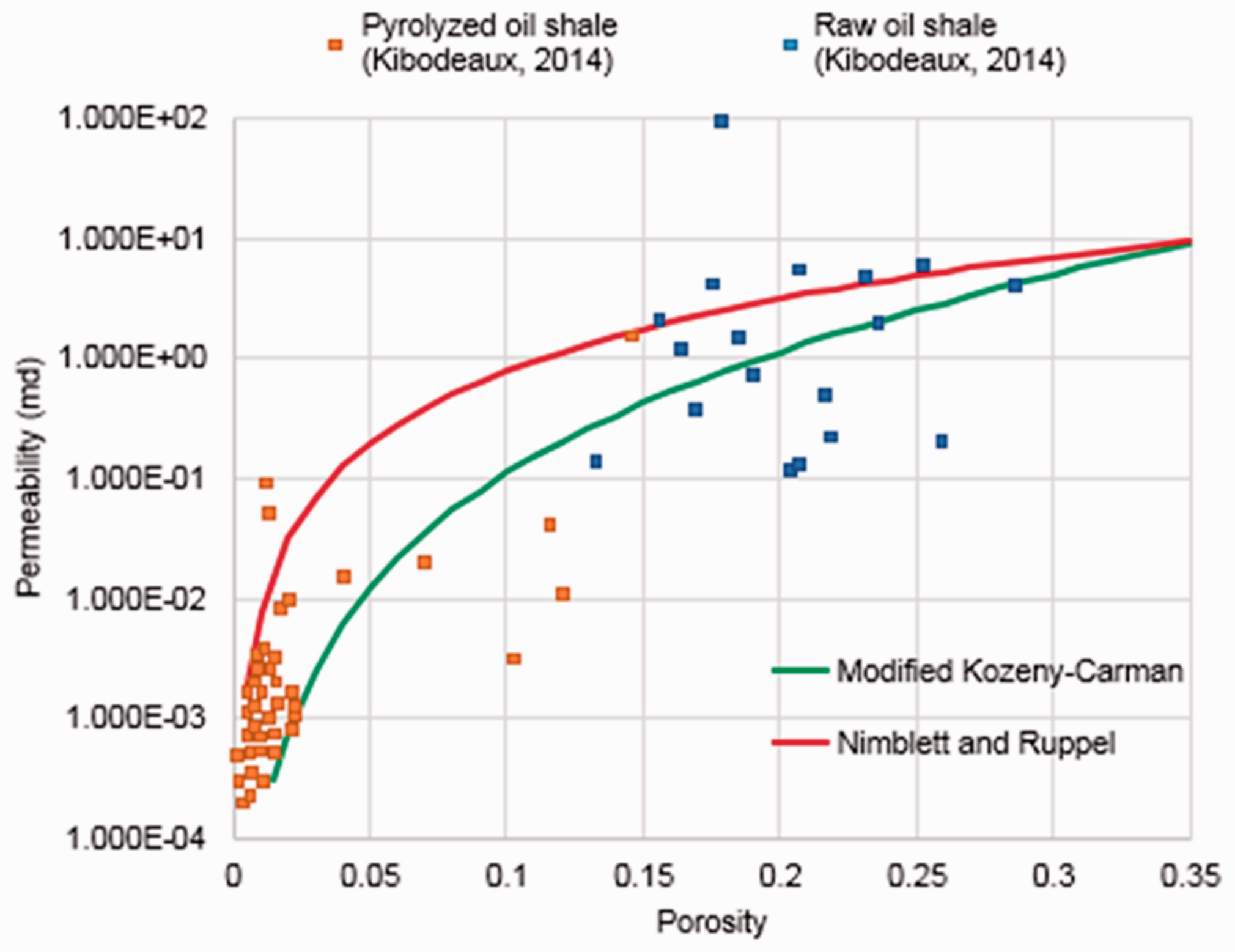
Delineation of general Shell ICP method.

Figure 2.

Correlations of porosity and permeability.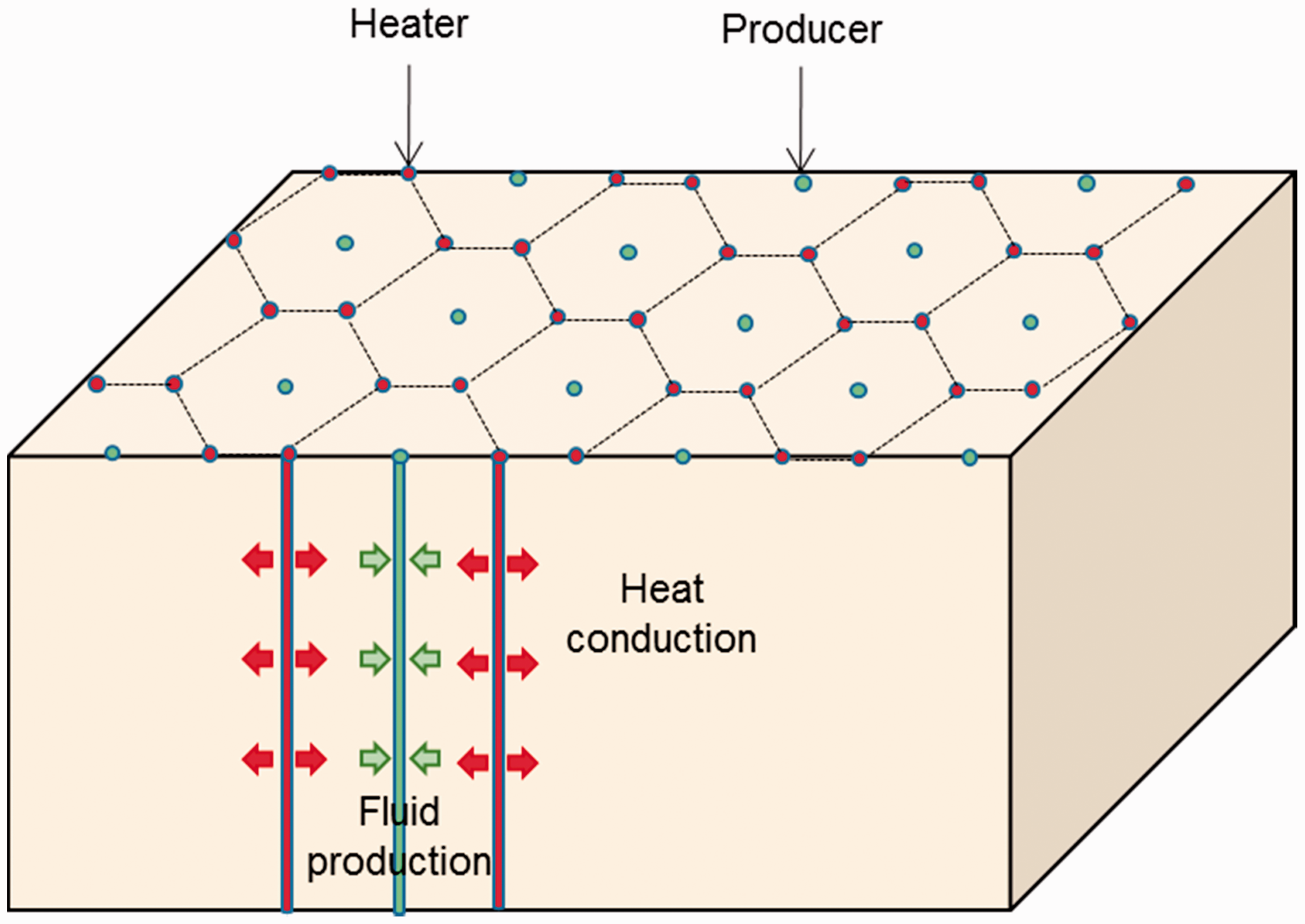

In the implementation of ICP, the initial saturation of fluid phases in oil shales, especially the amount of water, has the significant impact on the project efficiency by affecting flow of converted fluids. There have been several simulation studies on the ICP, but they did not consider the effect of differing water content in the system on the fluid flow in production process. Shen (2009) has conducted the simulation of pilot production by ICP in the Mahogany Field Experiment; heating and production processes after the 30 days of dewatering process have been simulated. Fan et al. (2010) have simulated the application of ICP using diverse heating temperatures and heater patterns; they have omitted the water component and aqueous phase in the simulations, and the effect of water in the system has been ignored.

Comparing with the ICP method of electrical heating, hot fluid injection can be considered to heat the oil shales by heat convection as well as conduction, especially in the systems with pre-existing fracture networks. Hot gas such as CO₂ and hot water are favorable to be injected to gas-dominant reservoirs and water-dominant reservoirs, respectively. Lee et al. (2016a) have conducted the comparison study of diverse in-situ upgrading processes including ICP and ExxonMobil Electrofrac of electrical heating, and Texas A&M Steamfrac of hot water injection to analyze the effect of heating methods on the productivity and product selectivity in the oil shale system initially filled with 100% aqueous phase. Youtsos et al. (2013) have conducted the numerical simulation of thermal and reaction fronts during the in-situ upgrading by hot CO₂ injection in the oil shale system initially filled with 100% gaseous phase.

From the previous simulation studies on the in-situ upgrading process, we have found that the effect of differing initial saturations of fluid phases, especially the water content, has not been considered thoroughly, even though it should be fully accounted for the realistic simulations. Also, the comparison of heating methods has not been done in the same geometry of reservoir system. In this regard, we conduct two sets of numerical simulations in this study.

The first set of simulations involves four cases of a five-spot well pattern problem to analyze the effects of heating methods and the initial saturations of fluid phases in the same reservoir geometry. In this set of simulation cases, we use the five-spot well pattern of simple geometry to clearly estimate and compare the system responses including the distributions of temperature, kerogen volume fraction, and effective porosity, and the production behaviors of fluid phases and components.

The second set of simulations involves three cases of ICP method as the application of actually proposed in-situ upgrading technology. We use the well patterns introduced in the pilot production of MDP-S in the Green River Formation of the United States (Fowler and Vinegar, 2009). From this set of simulation cases, we analyze the effect of water content on the implementation of ICP method in the two-phase-aqueous-and-gaseous reservoirs. In each simulation case, the system response, production behavior of fluids, product selectivity, and productivity will be analyzed.

Simulation model description

In the numerical simulation of in-situ upgrading process, heating and production procedures should be described thoroughly to predict the likelihood of feasible production of hydrocarbons from oil shales. However, the physical and chemical phenomena occurring in the thermal processes applied to oil shales are highly complex to be described, because they involve a number of subsequent/concurrent chemical reactions, continuous evolution of porosity and permeability, and changes of fluid composition and phase properties.

In this study, we use a fully functional simulator developed for the in-situ upgrading process, which describes the thermophysical and chemical phenomena in the oil shale reservoir systems (Lee et al., 2016b). The simulator is capable of describing the coupled flow of multiphase-multicomponent fluid and heat in porous and fractured media involving chemical reactions, where the porosity and permeability continuously alter by the changing amount of solid phase during the thermal process.

The simulator involves the six chemical reactions of in-situ upgrading process provided by Shell in the Green River Formation of the United States as listed in Table 1. The reactions are (1) kerogen decomposition, (2) cracking of heavy oil in gaseous phase, (3) cracking of heavy oil in liquid organic phase, (4) cracking of light oil in gaseous phase, (5) cracking of light oil in liquid organic phase, and (6) coking of hydrocarbon gas. Including nitrogen to the components in the reactions, 10 components of heavy oil (C₂₂H₄₆), light oil (C₁₁H₂₄), hydrocarbon gas (C₂H₆), water (H₂O), hydrogen (H₂), carbon dioxide (CO₂), nitrogen (N₂), kerogen, prechar, and char are considered in the four phases of aqueous, liquid organic, gaseous, and solid.

Table 1.

Chemical reactions of in-situ upgrading process.

Reaction	Chemical formula		Frequency factor (1/s)	Activation energy (J/mol)
Kerogen decomposition	Kerogen →	0.02691 H₂O + 0.009815 heavy oil + 0.01755 light oil + 0.0402 HC gas + 0.01049 H₂ + 0.0541 CO₂ + 0.5828 prechar	4.34 × 10⁷	161 600
Cracking of heavy oil	Heavy oil (G) → Heavy oil (O) →	0.2034 light oil + 2.1153 HC gas + 16.9188 prechar 1.8269 light oil + 0.0402 HC gas + 1.8735 prechar	9.20 × 10¹¹ 9.20 × 10¹¹	206 034 206 034
Cracking of light oil	Light oil (G) → Light oil (O) →	5.1983 HC gas 0.5125 HC gas + 11.0771 prechar	6.77 × 10¹¹ 6.77 × 10¹¹	219 328 219 328
Coking of hydrocarbon gas	HC gas (G) →	3.0 H₂ + 1.8885 char	8.87 × 10¹⁵	311 432

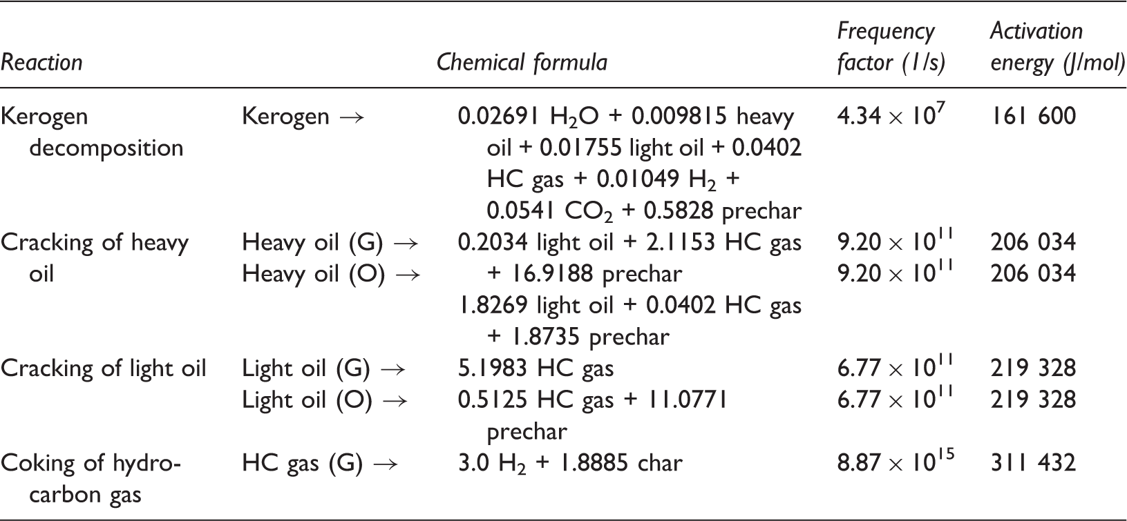
Source: Wellington et al. (2005).

Materials in the reservoir system present as in either single-phase or multiphase-equilibrium states by the thermophysical conditions. Phase transition by fluid flow, change of reservoir pressure or temperature, chemical reactions, vaporization, condensation, and gas evolution is considered. The simulator computes the thermodynamic properties of phases by diverse equations of state and mixing rules. The properties of bulk oil shale rock are computed by considering the composition of phases in its pores and fractures.

Many oil shales are composed of dolomite and calcine, and natural fracture systems occur in such systems (Dyni, 2006). The simulator describes the naturally fractured media using the concept of Multiple Interacting Continua (MINC) (Pruess, 1985). MINC simulates the fractured rock by dividing the domain into homocentric grids for the fracture at the external position and the rock matrix at the internal position. The fracture domain mainly provides the flowing path of fluid and heat. In our simulations, the reservoir contains a well-connected natural fracture system with the dense fracture spacing of 3 m and the high fracture permeability of 1.480 × 10⁻¹³ m² (= 150 md), and it satisfies the assumption of MINC method, which considers the naturally fractured reservoir as a continuum. We use the volumetric fraction of 0.01 of bulk oil shale rock for the fracture network.

Continuous change of porosity and permeability of rock matrix is computed at every moment by accounting kerogen decomposition, subsequent generation of fluids and solids, fluid expansion by the increase of pressure and temperature during the heating process, and pressure decrease by production. Two concepts of porosities are accounted in the simulations—media porosity and effective porosity. Media porosity involves whole phases of fluids and solid, while effective porosity involves only fluid phases. The permeability of rock is computed every moment according to the evolution of effective porosity.

In our two sets of simulation case study, we examine the effects of initial saturation of fluid phases in the pores and fractures and the diverse heating methods. In the first set of five-spot well pattern problems, we conduct four cases of simulations in the reservoir filled with single-phase fluid initially—electrical heating in the single-phase-aqueous reservoir, electrical heating in the single-phase-gaseous reservoir, hot water injection in the single-phase-aqueous reservoir, and hot CO₂ injection in the single-phase-gaseous reservoir. In the second set of ICP problems, we conduct three cases of simulations in the reservoir filled with two-phase-aqueous-and-gaseous fluids with different water contents to each other—S_iA = 0.16, 0.44, and 0.72 (S_iG = 0.84, 0.56, and 0.28).

As well as the different initial saturation of fluid phases and the diverse heating methods, we use the different irreducible saturations of phases, different correlation models of porosity and permeability, and different initial effective porosity between the two sets of problems. Their conditions of the five-spot well pattern problems have been obtained from the validated model of previous study (Lee et al., 2016b). First, in the set of five-spot well pattern problems, we use the irreducible saturations of S_iA = 0.30, S_iO = 0.20, and S_iG = 0.05 at the matrix domain, and S_iA = 0.03, S_iO = 0.02, and S_iG = 0.005 at the fracture domain, respectively; in the set of ICP problems, we use the smaller irreducible saturations of S_iA = 0.16, S_iO = 0.12, and S_iG = 0.04 at the matrix domain, and S_iA = 0.016, S_iO = 0.012, and S_iG = 0.004 at the fracture domain, respectively, to counterbalance the flow of two-phase fluid presenting initially. Second, we use different correlation models of porosity and permeability in the two sets of problems as shown in Figure 2, even both models are based on the core data of Green River Formation (Kibodeaux, 2014). In the set of five-spot well pattern problems, we use the correlation of Nimblett and Ruppel (2003), which was used in the validated model of previous study (Lee et al., 2016b); in the set of ICP problems, we use the modified Kozeny–Carman equation for the better representation of core data (Krauss and Mays, 2014). Third, in the set of five-spot well pattern problems, we use the initial effective porosity of 0.04 and corresponding absolute permeability of 1.228 × 10⁻¹⁶ m² (= 0.124 md) at the rock matrix; in the set of ICP problems, we use the initial effective porosity of 0.015 and 3.092 × 10⁻¹⁹ m² (=3.133 × 10⁻⁴ md) at the rock matrix, for more realistic description of low-permeable raw shales.

Simulation of five-spot well pattern problems

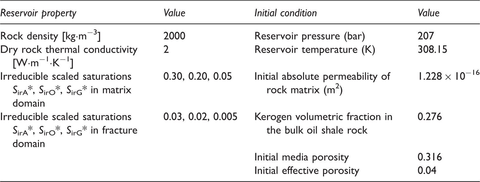
Simulation model and initial reservoir properties

A quarter of a five-spot well pattern system in a well-connected naturally fractured reservoir is simulated by using a 2D model with 1 m thickness (Figure 3). The heater (or the injection well) is located at the corner of the model, and the production well is located at the other corner on a diagonal line. The reservoir properties and the initial conditions have been obtained from the Green River Oil Shale, as provided in Table 2 (Lee et al., 2016b). Two initial conditions of fluid phases have been considered—single phase aqueous and single phase gaseous. The initial aqueous phase and gaseous phase are occupied by 100% of water component and 100% of CO₂, respectively. For the computation of relative permeability and capillary pressure in the matrix domain, Van Genuchten model and Parker’s model have been used for the two-phase flow and the three-phase flow, respectively.

Figure 3.

Reservoir geometry and simulation model of five-spot well pattern cases.

Table 2.

Reservoir properties and initial conditions in the simulation cases of five-spot well pattern problems.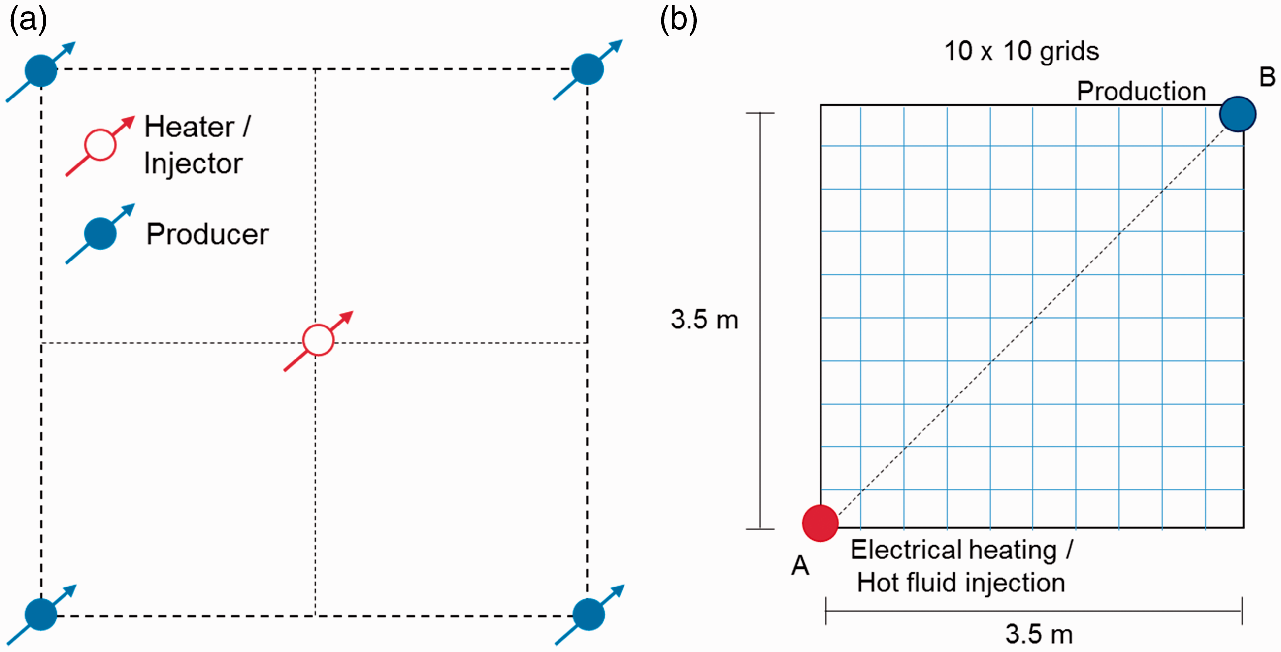

Reservoir property	Value	Initial condition	Value
Rock density [kg·m⁻³]	2000	Reservoir pressure (bar)	207
Dry rock thermal conductivity [W·m⁻¹·K⁻¹]	2	Reservoir temperature (K)	308.15
Irreducible scaled saturations S_irA, S_irO, S_irG* in matrix domain	0.30, 0.20, 0.05	Initial absolute permeability of rock matrix (m²)	1.228 × 10⁻¹⁶
Irreducible scaled saturations S_irA, S_irO, S_irG* in fracture domain	0.03, 0.02, 0.005	Kerogen volumetric fraction in the bulk oil shale rock	0.276
		Initial media porosity	0.316
		Initial effective porosity	0.04

Four cases of thermal and production processes for 1000 days are simulated—electrical heating in the aqueous phase reservoir, electrical heating in the gaseous phase reservoir, hot water injection in the aqueous phase reservoir, and hot CO₂ injection in the gaseous phase reservoir. In the cases of electrical heating by an electric heater, the heater grid block is continuously heated during the whole process of heating and production, and the constant heater temperature of 618.15 K is used. In the cases of hot fluid injection, the heated fluids are injected by the constant rate of 5 × 10⁻⁴kg/s in the simulation model (= 2 × 10⁻³kg/s in one five-spot well pattern system), and by the variable enthalpy that makes the injection fluid temperature = 618.15 K. The heater/injection well temperature for each case during the process is provided in Figure 4. It shows that the heater temperature in the electrical heating cases was kept constant from t = 0 days to t = 1000 days by the constant temperature at the heater well grid, while the injection well temperature in the cases of hot fluid injection was gradually increasing from the initial reservoir temperature to the objective temperature. The injection well temperature approached the objective temperature of 618.15 K at t = 400 days in the injection cases.

Figure 4.

Temperature of the heater/injection well of five-spot well pattern cases.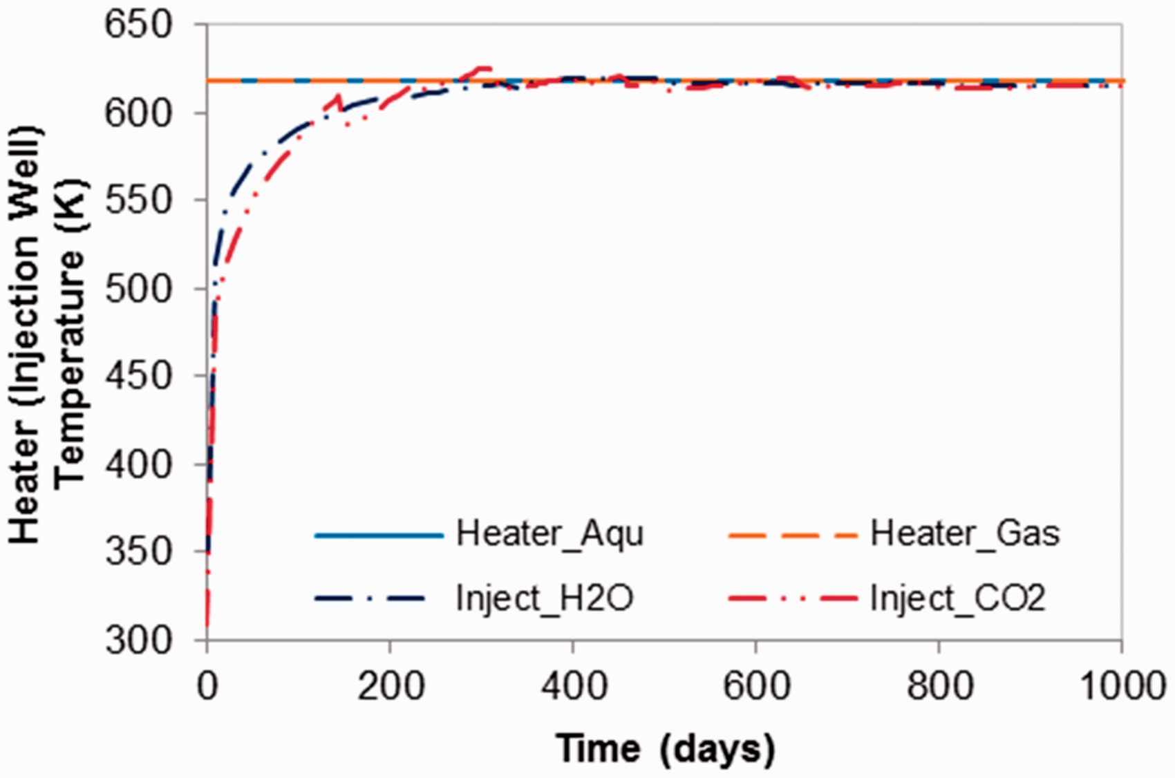

From t = 0 days to 50 days, only thermal process is applied in the cases of electrical heating, while the same rate of fluid to the injection rate is produced in the cases of hot fluid injection. Then the converted fluids are produced from t = 50 days to 1000 days in each case using the gradually decreasing wellbore flowing pressure.

Simulation results and discussion

System behavior

The distributions of temperature on the diagonal line AB in Figure 3 during the heating and production processes are provided in Figure 5. The case of hot water injection shows the fastest temperature increase among the cases. This has been caused by that the flowing hot water has allowed the heat to be transferred more vigorously by convection, than the cases of electrical heating. Comparing with the case of hot CO₂ injection, hot water has the higher heat capacity than hot CO₂ of same temperature; thus the hot water injection case shows even faster temperature increase in the reservoir than the hot CO₂ injection case.

Figure 5.

Reservoir profiles of five-spot well pattern cases—distributions of temperature on the line AB.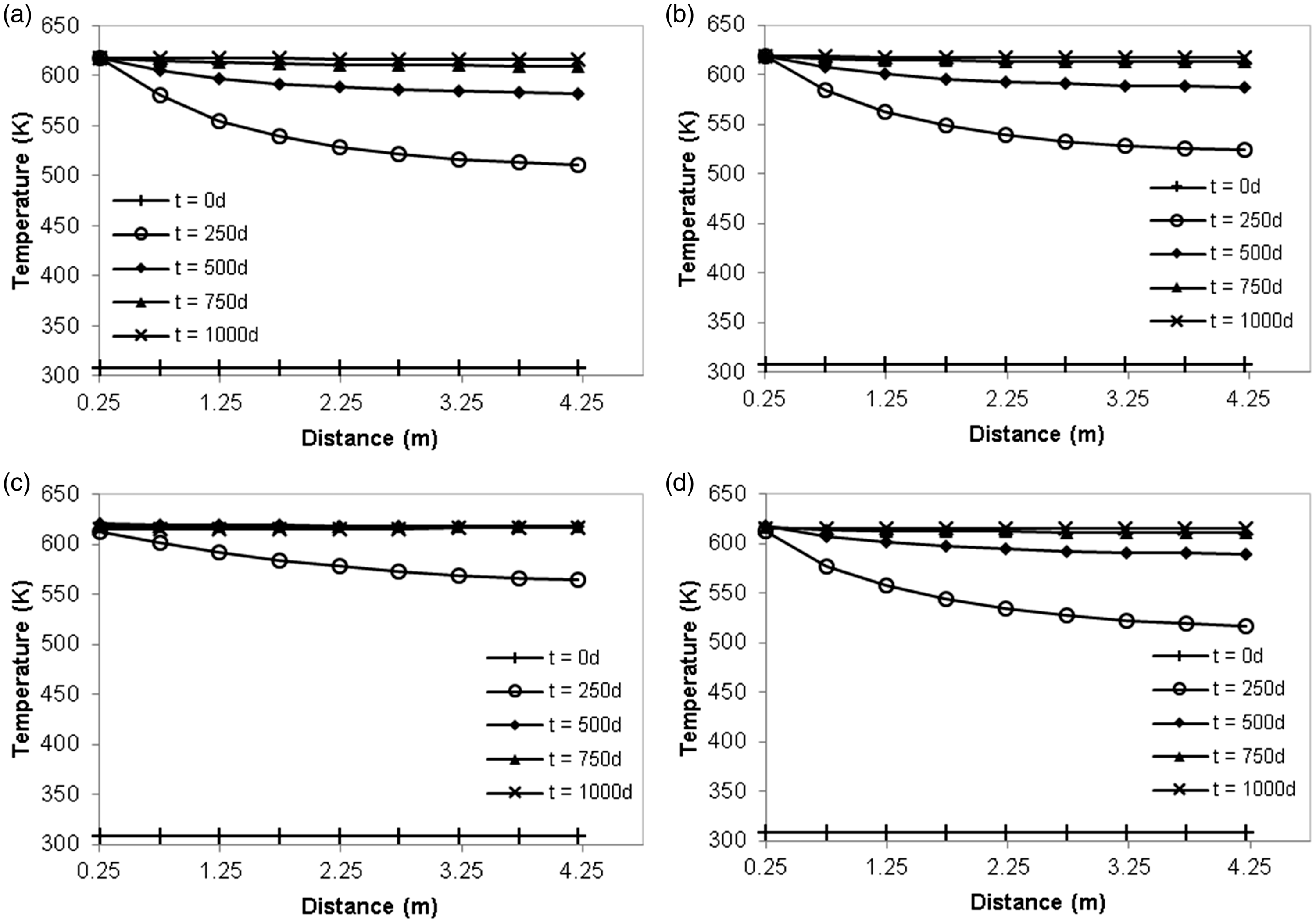

Figure 6 shows the distributions of kerogen volume fraction in solid phase. By the fast increase of temperature, the case of hot water injection shows the active kerogen decomposition in the wide area from the early time of 250 days. The distributions of effective porosity of the matrix domain are provided in Figure 7. The case of hot water injection has the fastest increase of effective porosity in the wide area among the cases, by the fast increase of temperature and the active decomposition of kerogen. At the end of the process at t = 1000 days, the effective porosity in each case have approached 0.2.

Figure 6.

Reservoir profiles of five-spot well pattern cases—distributions of kerogen volume fraction in solid phase on the line AB.

Figure 7.

Reservoir profiles of five-spot well pattern cases—distributions of effective porosity on the line AB.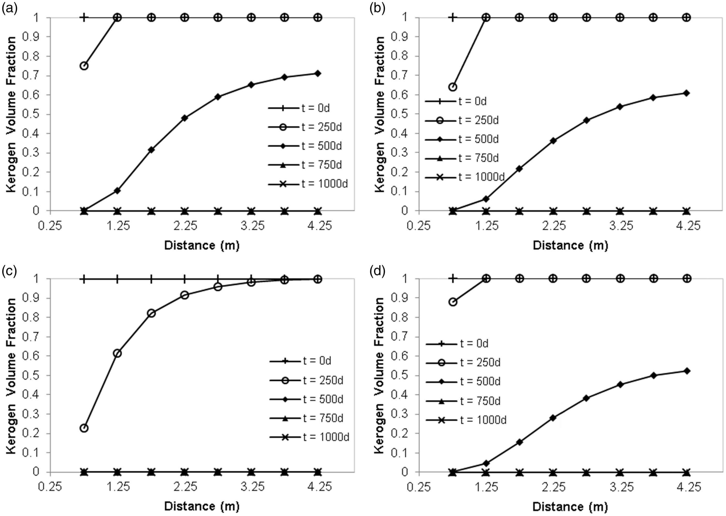

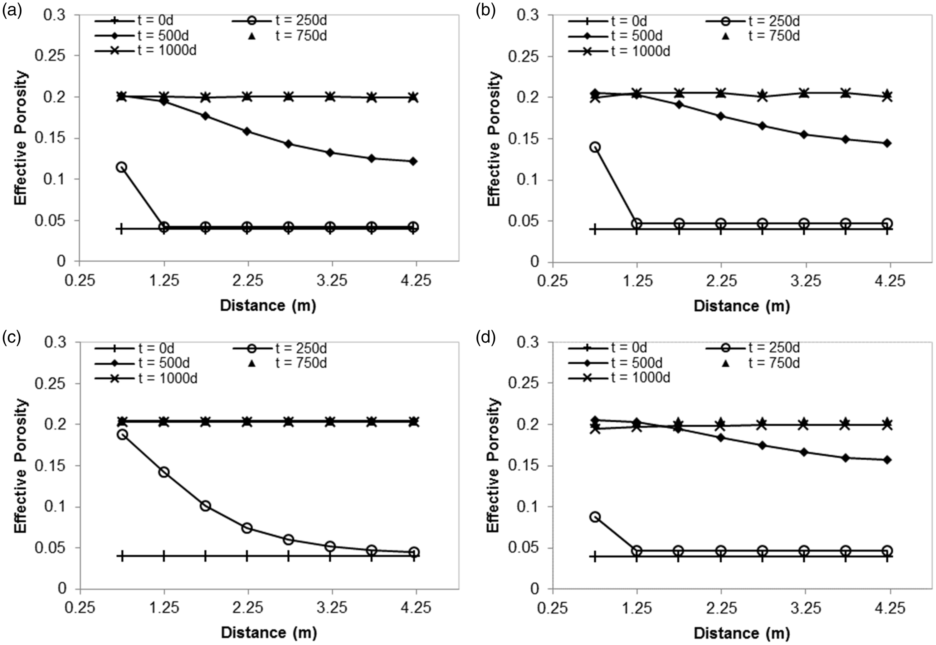
The increase of effective porosity in each case during the processes of heating and production has been resulted by the kerogen decomposition and fluid expansion, but the final effective porosity is still smaller than the initial media porosity of 0.316 because of the generation of solid products. In the cases of electrical heating and hot CO₂ injection in the gaseous phase reservoir, it is found that the effective porosity of the matrix domain at distance = 0.75 m at t = 750 days is higher than the final effective porosity. This has been caused by that the increase of effective porosity by the gaseous phase expansion in the matrix domain at t = 750 days is higher than that at t = 1000 days in those cases, by the higher reservoir pressure at t = 750 days.

Kerogen mass in place and productions of phases

Figure 8 provides the kerogen mass in place and the production rates of phases in one five-spot well pattern system in the simulation cases. In Figure 8(a), it is found that the kerogen mass in place rapidly decreases from t = 400 days, 370 days, 200 days, and 370 days, until it reaches to zero at t = 750 days, 710 days, 470 days, and 710 days, in the cases of electrical heating in the aqueous phase reservoir, electrical heating in the gaseous phase reservoir, hot water injection in the aqueous phase reservoir, and hot CO₂ injection in the gaseous phase reservoir, respectively.

Figure 8.

Results of five-spot well pattern cases—kerogen mass in place and production rates of phases.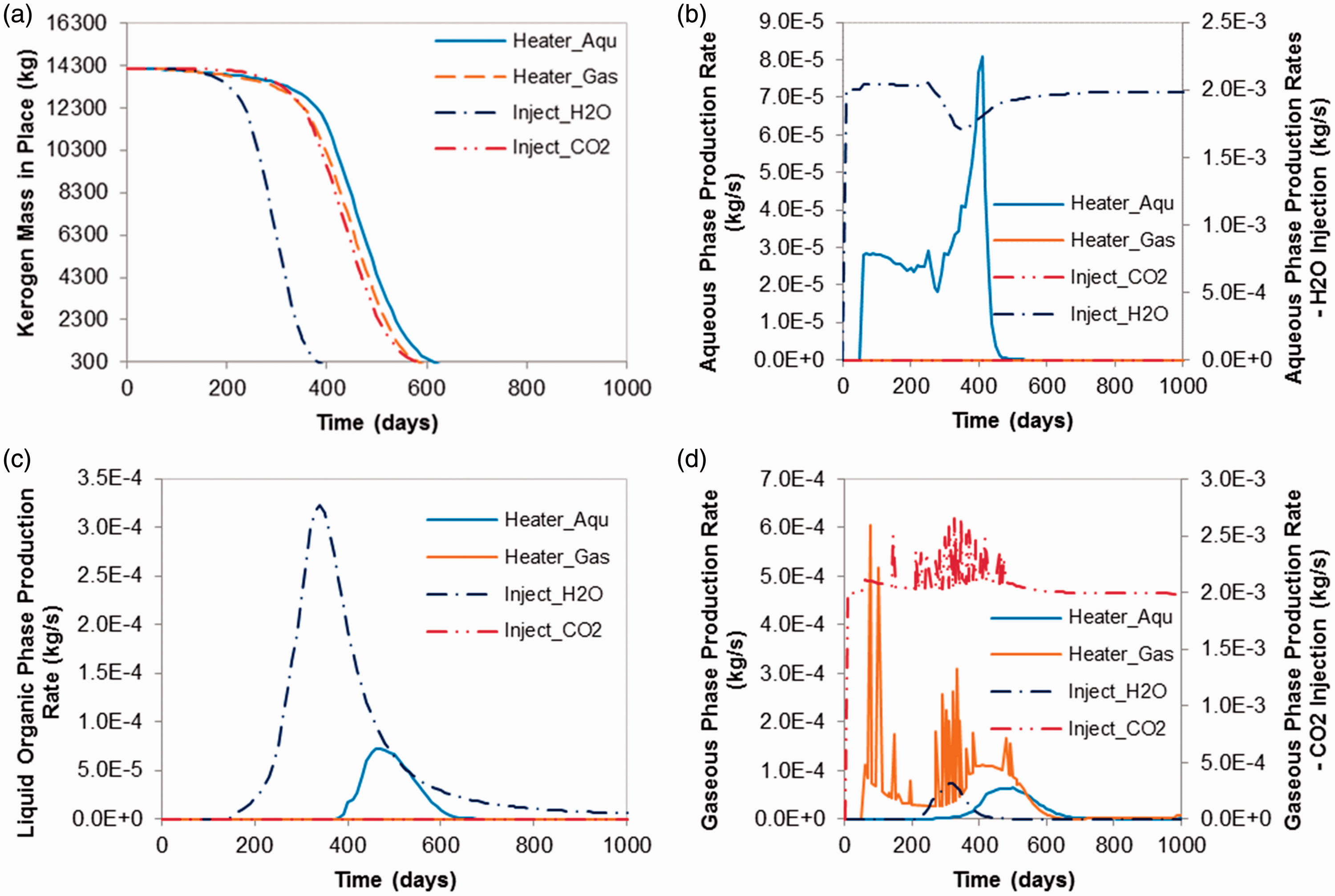

Figure 8(b) and (c) show that aqueous phase and liquid organic phase are not produced in the cases of electrical heating and hot CO₂ injection in the gaseous phase reservoir during the process, and they have remained at the matrix domain after being generated from the kerogen decomposition due to their far lower mobility than that of gaseous phase in such system where gaseous phase is dominant.

In Figure 8(b), it is found that the peak of the production rate of aqueous phase is 8.103 × 10⁻⁵kg/s (= 0.0587 STB/day) at t = 410 days in the case of electrical heating in the aqueous phase reservoir. In the case of hot water injection in the aqueous phase reservoir, the aqueous phase production rate remains almost same as the injection rate after t = 600 days.

In Figure 8(c), it is found that the peaks of the production rate of liquid organic phase are 7.267 × 10⁻⁵kg/s (= 0.0702 STB/day) and 3.229 × 10⁻⁴kg/s (= 0.312 STB/day) in the cases of electrical heating in the aqueous phase reservoir and hot water injection in the aqueous phase reservoir, respectively.

From Figure 8(d), it is found that the cases of electrical heating and hot CO₂ injection in the gaseous phase reservoir have much higher production rate of gaseous phase production than the cases of aqueous phase reservoir. The peaks of the gaseous phase production rate are 6.458 × 10⁻⁵kg/s (= 0.179 MSCF/day) at t = 500 days and 7.287 × 10⁻⁵kg/s (= 0.202 MSCF/day) at t = 320 days in the cases of electrical heating and hot water injection in the aqueous phase reservoir, respectively. In the case of electrical heating in the gaseous phase reservoir, the peak of gaseous phase production rate is 6.053 × 10⁻⁴kg/s (= 1.679 MSCF/day) at t = 60 days. In the case of hot CO₂ injection in the gaseous phase reservoir, the gaseous phase production rate peaks at t = 360 days by the rate of 2.511 × 10⁻³kg/s (= 6.965 MSCF/day) and remains almost same as the injection rate after t = 500 days. The cumulative productions of phases are summarized in Table 3.

Table 3.

Cumulative productions of phases in the five-spot well pattern problems.

Cases	Aqueous production (kg)	Liquid organic production (kg)	Gaseous production (kg)	GOR (kg/kg)	WOR (kg/kg)
Electrical heating/aqueous phase reservoir	1082.43	815.08	1087.02	1.334	1.328
Electrical heating/aqueous phase reservoir	(9.08 STB)	(9.11 STB)	(42.23 MSCF)
Electrical heating/gaseous phase reservoir	0	0	3789.81	–	–
Electrical heating/gaseous phase reservoir			(147.22 MSCF)
Hot water injection/aqueous phase reservoir	1.689 × 10⁵	5062.01	691.72	0.137	33.36
Hot water injection/aqueous phase reservoir	(1416.22 STB)	(56.60 STB)	(26.87 MSCF)
Hot CO₂ injection/gaseous phase reservoir	0	0	1.779 × 10⁵	–	–
Hot CO₂ injection/gaseous phase reservoir			(6909.49 MSCF)

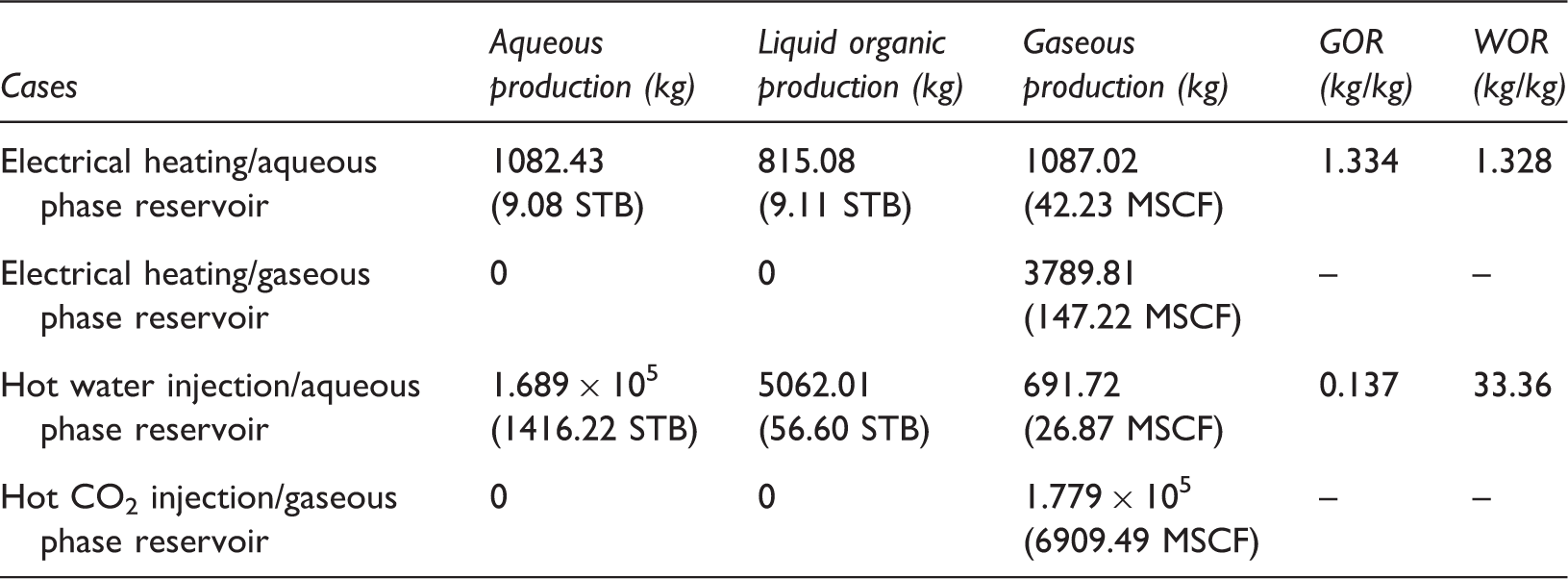
GOR: gaseous phase–liquid organic phase; WOR: aqueous phase–liquid organic phase.

Productions of components

The production rates of fluid components are provided in Figure 9, and the cumulative productions of components are listed in Table 4. From Figure 9(a), (b), and (f), it is found that the heavy oil, light oil, and water components are produced in the cases of electrical heating and hot CO₂ injection in the gaseous phase reservoir, even though liquid organic phase and aqueous phase have not been produced in those cases as shown in Figure 8. In these cases, those components are produced in the form of vapor in gaseous phase.

Figure 9.

Results of five-spot well pattern cases—production rates of components.

Table 4.

Cumulative productions of components in the five-spot well pattern problems.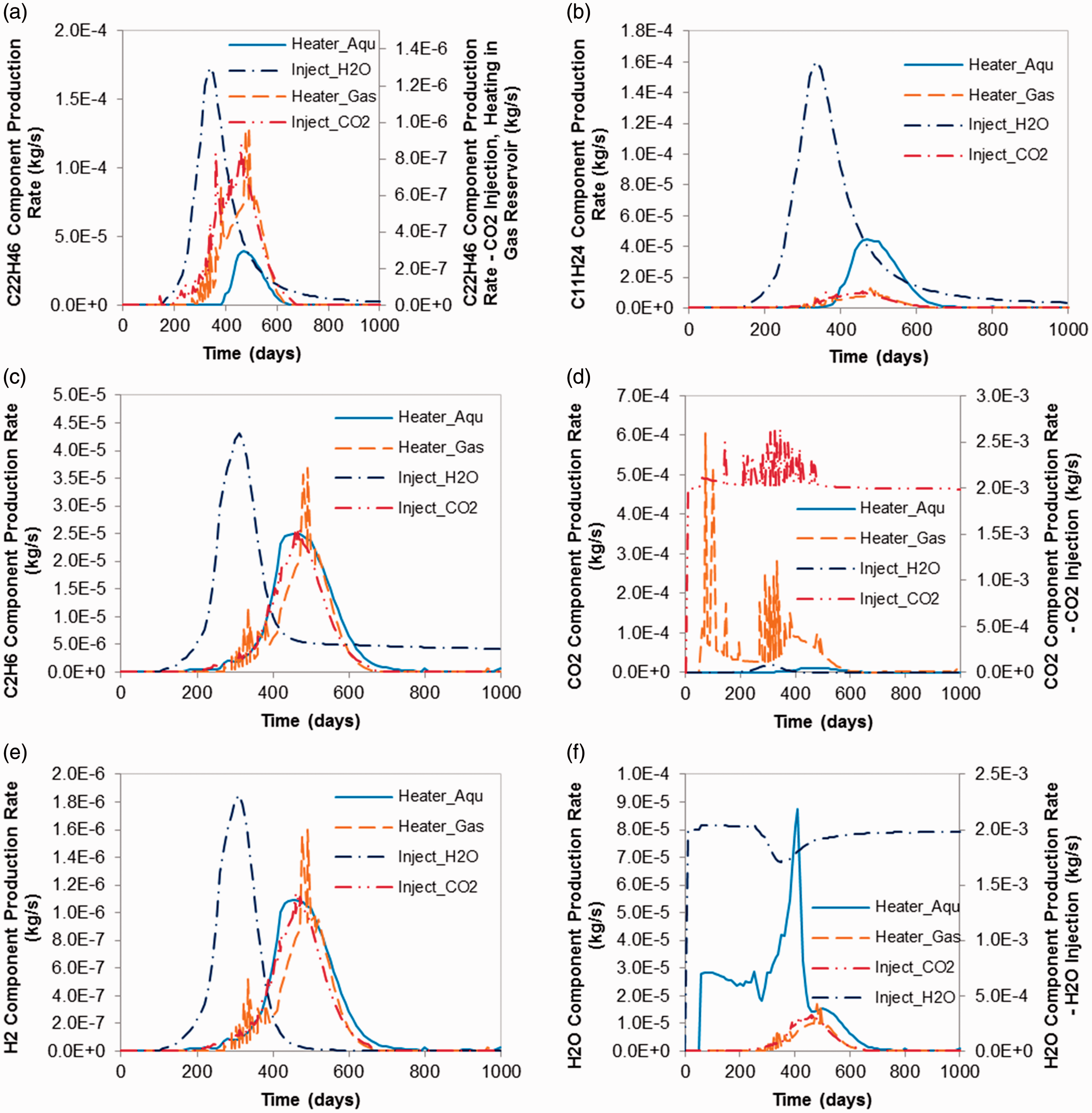

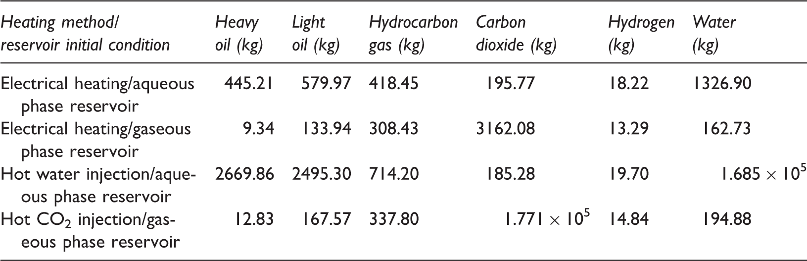
Heating method/ reservoir initial condition	Heavy oil (kg)	Light oil (kg)	Hydrocarbon gas (kg)	Carbon dioxide (kg)	Hydrogen (kg)	Water (kg)
Electrical heating/aqueous phase reservoir	445.21	579.97	418.45	195.77	18.22	1326.90
Electrical heating/gaseous phase reservoir	9.34	133.94	308.43	3162.08	13.29	162.73
Hot water injection/aqueous phase reservoir	2669.86	2495.30	714.20	185.28	19.70	1.685 × 10⁵
Hot CO₂ injection/gaseous phase reservoir	12.83	167.57	337.80	1.771 × 10⁵	14.84	194.88

Comparing Figure 9(d) and (f) with the Figure 8(b) and (d), it is found that the aqueous phase and gaseous phase are composed of almost 100% water and 100% CO₂ in the cases of hot water injection in the aqueous phase reservoir and hot CO₂ injection in the gaseous phase reservoir, respectively. From Table 4, it is found that the case of hot water injection in the aqueous phase reservoir shows the highest cumulative production of every fluid component except for CO₂, which shows the highest value of cumulative production in the case of hot CO₂ injection.

Simulation of ICP

Simulation model and initial reservoir properties

The simulation examples include the three cases having the diverse water contents in the reservoir systems. The three reservoirs are naturally fractured and initially filled with two phases of fluid—aqueous and gaseous. The initial volume fraction of the aqueous phase in the void spaces of pores and fractures are 0.16, 0.44, and 0.72 in case 1, case 2, and case 3, respectively. The initial aqueous phase and gaseous phase are occupied by 100% of water component and 100% of hydrocarbon gas, respectively. The effects of initial saturation of aqueous phase on the productivity and product selectivity are evaluated through the simulation cases.

In the simulation cases, electrical heating by multiple electric heaters of ICP has been applied, with the specific well patterns proposed by MDP-S pilot production in Green River Formation (Fowler and Vinegar, 2009). Multiple electric heaters and producers are located in hexagonal patterns in the reservoir (Figure 10(a) and (b)). A quarter of one hexagon has been simulated using a 2D model as shown in Figure 10(c), which has 34.4 m thickness as in the pilot production implementation. The closed boundary condition for the flows of heat and fluid has been applied at the boundaries. In the simulations, heating and production are continued until t = 300 days. The electric heaters are heated up to T = 618.15 K (=345℃). The converted fluids by the heating process are produced using the gradually decreasing wellbore flowing pressure.

Figure 10.

Reservoir configuration and simulation model of ICP cases.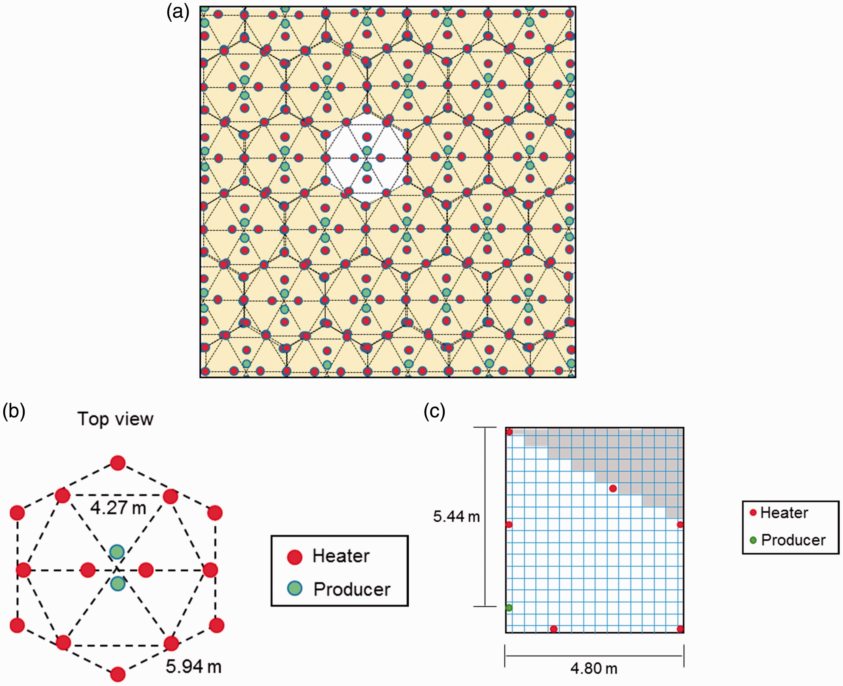

The reservoir properties and the initial conditions are provided in Table 5. The reservoir rock properties and the initial conditions of reservoir including pressure and temperature are same to the previous cases of five-spot well pattern problems. The initial saturation of solid phase is 0.276, which is fully composed of kerogen. The initial effective porosity is 0.015 in each case, which corresponds to the initial absolute permeability of 3.133 × 10⁻⁴ md. For the computation of relative permeability and capillary pressure in the matrix domain, Van Genuchten model and Parker’s model have been used for the two-phase flow and the three-phase flow, respectively.

Table 5.

Reservoir properties and initial conditions in the simulation cases of ICP.

Reservoir property	Value	Initial condition	Value
Irreducible scaled saturations S_irA, S_irO, S_irG* in matrix domain	0.16, 0.12, 0.04	Initial absolute permeability of rock matrix (m²)	3.092 × 10⁻¹⁹ (=3.133 × 10⁻⁴ md)
Irreducible scaled saturations S_irA, S_irO, S_irG* in fracture domain	0.016, 0.012, 0.004	Kerogen volumetric fraction in the bulk oil shale rock	0.276
		Initial media porosity	0.291 0.015
		Initial effective porosity	0.291 0.015

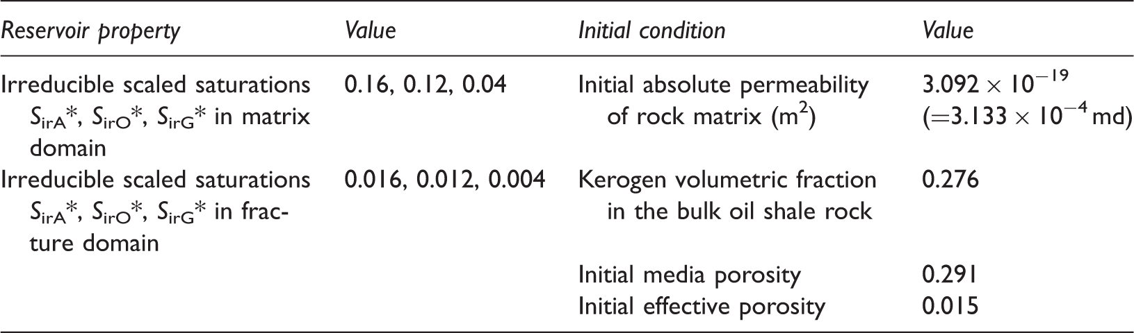
ICP: in-situ conversion process.

Simulation results and discussion

System behavior

The distribution profiles of temperature and kerogen mass in place during the process in case 1 are shown in Figure 11. The formation temperature increases gradually from region around the heaters and approaches evenly high temperature at t = 230 days. The kerogen in the system gradually decomposes from the region around the heaters, and whole decomposes at t = 230 days. Cases 2 and 3 have showed the similar distribution profiles to case 1.

Figure 11.

Reservoir profiles of ICP case 1.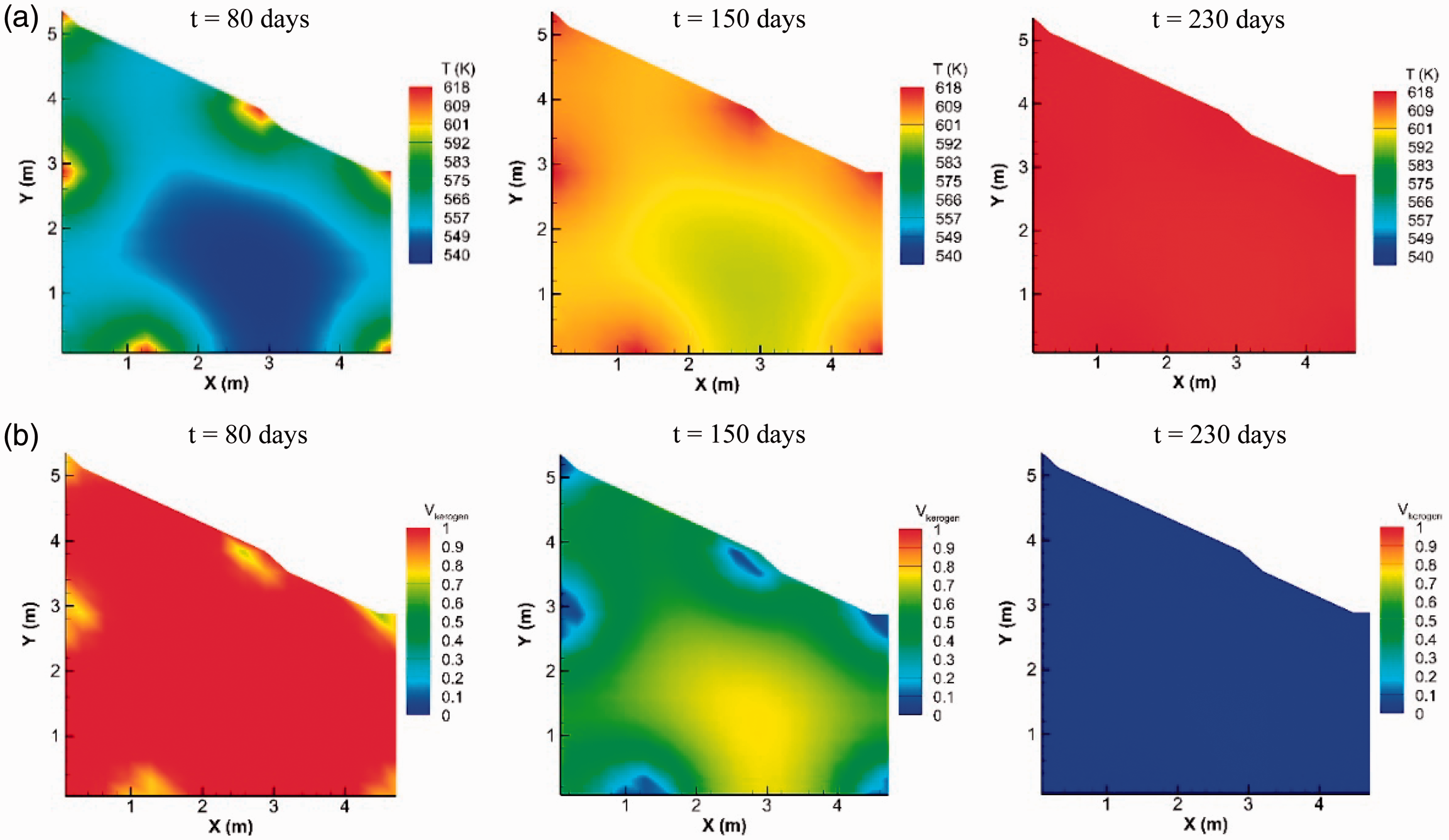

The system responses of each case are shown in Figure 12. Oil shale formation of 34.44 m interval has been considered. Figure 12(a) shows that kerogen in the system actively decomposes from t = 100 days in each case. The curves of kerogen mass in place show insignificant difference among the cases. This is because, the initial volume fraction of void space of pores and fractures was 0.025, and the difference of thermal conductivity of bulk shale is less than 2% between the cases considering the following composite thermal conductivity of bulk oil shale rock.

K = (1 - φ) K_{R} + \sum_{β \equiv A, O, G, S} φ S_{β} K_{β}

(1)

where K_R and

K_{β}

are the thermal conductivities of dry porous rock and phase β [W·m⁻¹·K⁻¹], respectively.

Figure 12.

System behavior of ICP cases—kerogen mass in place in the system, and effective porosity and absolute permeability of rock matrix at the monitoring point (x, y) = (2.56 m, 2.56 m).

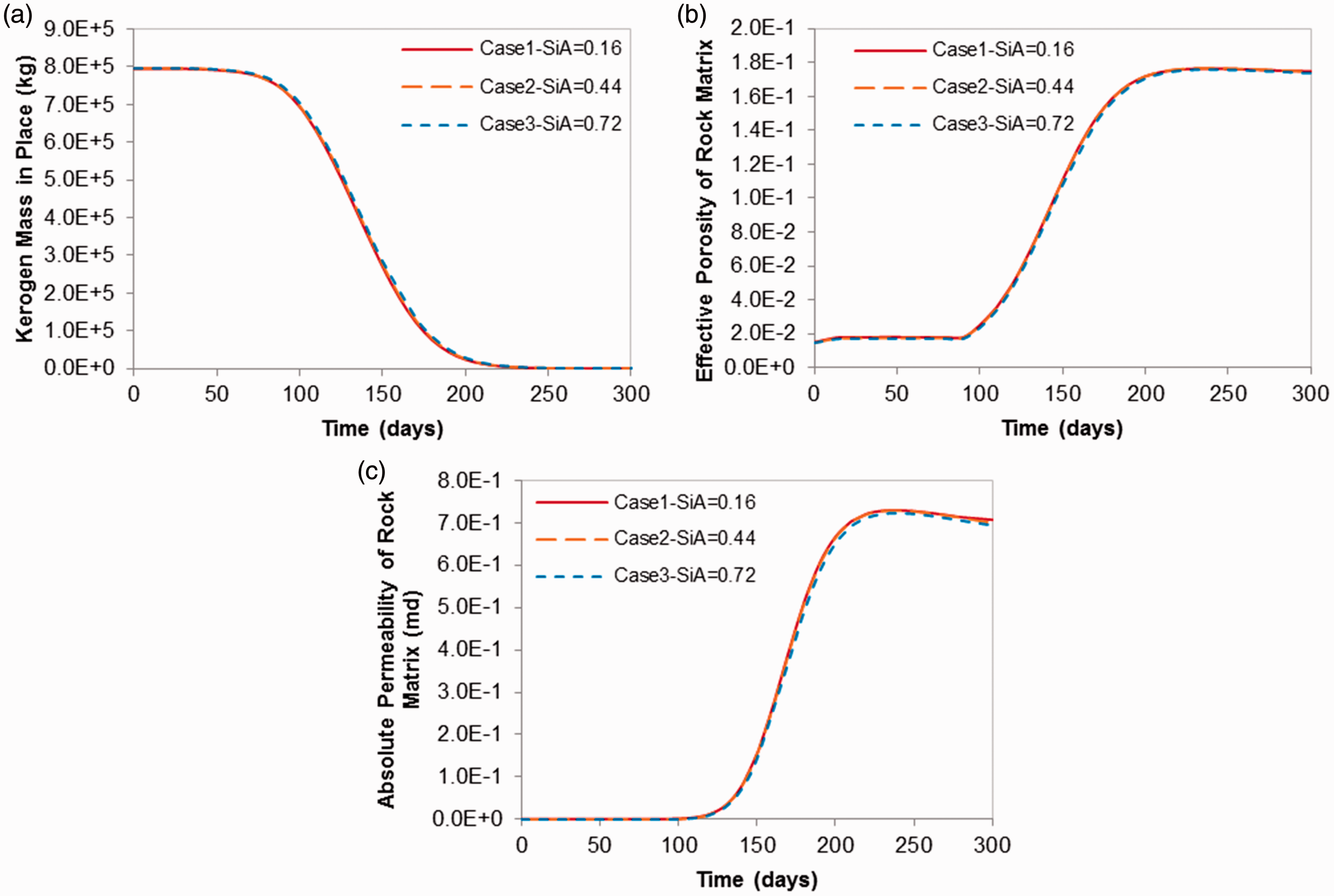
Figure 12(b) and (c) indicate the evolution of effective porosity and corresponding matrix permeability by the kerogen decomposition at the monitoring point (x, y) = (2.56 m, 2.56 m). The values of final effective porosity are 0.1748, 0.1742, and 0.1739 in the cases, respectively. They are smaller than the initial media porosity of 0.291 because of the solid products remaining in the pores. The effective porosity and matrix permeability slightly decrease from t = 220 days because the system pressure decreases due to the production, while temperature has stopped increasing.

Production of phases

Production is continued from t = 15 days to t = 300 days in each case. The production rates and cumulative productions of fluid phases are provided in Figure 13. In each case, the production rates of liquid organic phase and gaseous phase increase as kerogen actively decomposes, and gradually decreases after their peaks as the supply of hydrocarbons from kerogen decomposition decreases. The production rates of aqueous phase and liquid organic phase approach zero around t = 150 days and t = 250 days, respectively. After t = 250 days, only a small amount of gaseous phase is produced.

Figure 13.

Results of ICP cases—production rates and cumulative productions of fluid phases.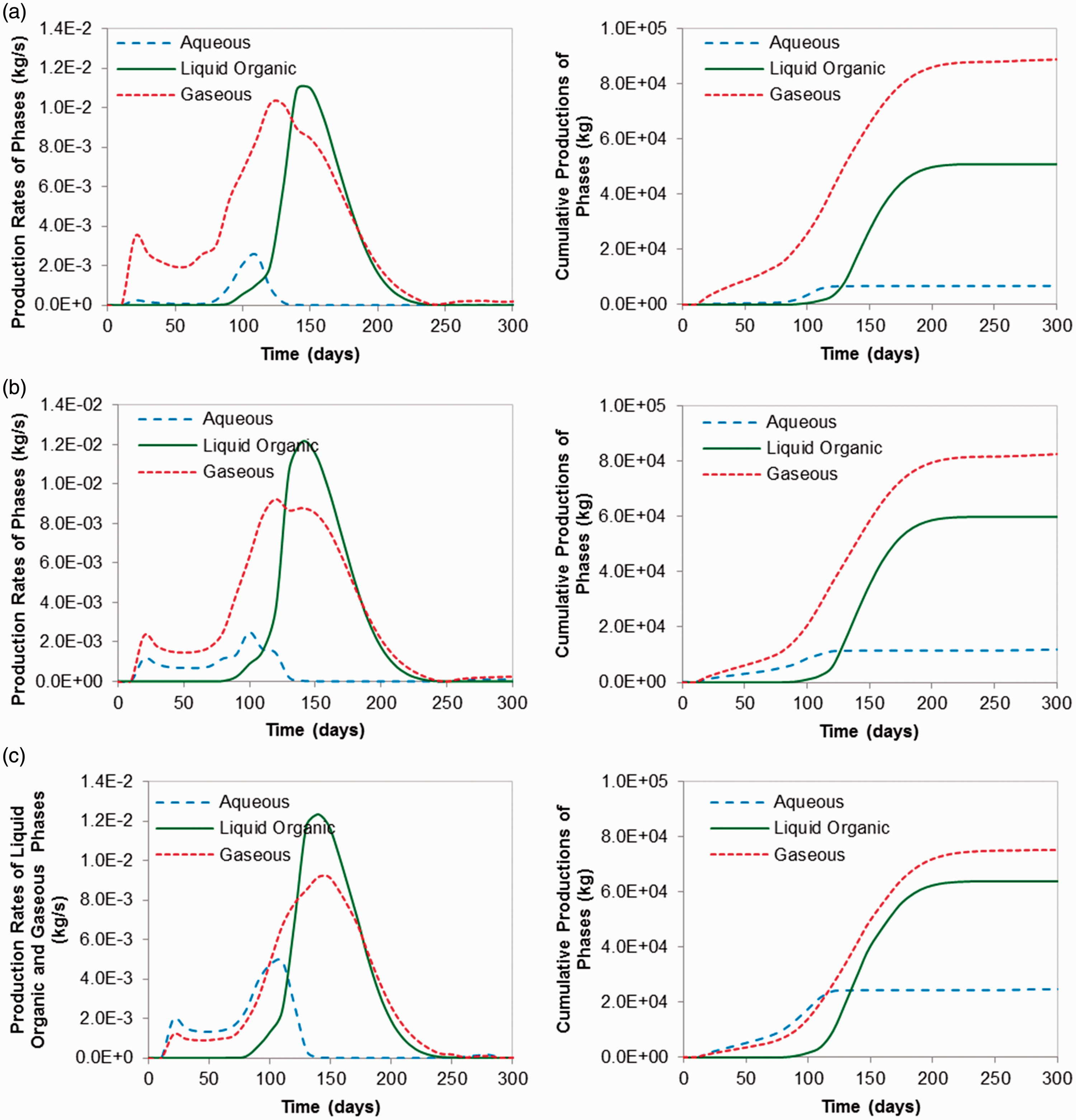

Production rate of liquid organic phase shows the highest peaks in each case, and gaseous phase and aqueous phase follow it. The peaks of the production rate of liquid organic phase are 1.100 × 10⁻²kg/s, 1.216 × 10⁻²kg/s, and 1.234 × 10⁻²kg/s; the peaks of the production rates of gaseous phase are 1.021 × 10⁻²kg/s, 9.252 × 10⁻³kg/s, and 9.204 × 10⁻³kg/s; the peaks of the production rates of aqueous phase are 2.566 × 10⁻³kg/s, 2.484 × 10⁻³kg/s, and 4.863 × 10⁻³kg/s in cases 1, 2, and 3, respectively. It is noticeable that case 2 with S_iA = 0.44 has the lower peak of the production rate of aqueous phase than case 1 with S_iA = 0.16, by the higher production rate of liquid organic phase.

The cumulative productions of fluid phases and the produced mass ratios of gaseous phase–liquid organic phase (GOR) and aqueous phase–liquid organic phase (WOR) are summarized in Table 6. The cumulative production of liquid organic phase increases with increasing initial saturation of aqueous phase, but the WOR also increases. The cumulative production of gaseous phase shows the highest value among the phases in every case.

Table 6.

Cumulative productions of phases in the ICP cases.

Cases	Aqueous production (kg)	Liquid organic production (kg)	Gaseous production (kg)	GOR (kg/kg)	WOR (kg/kg)
Case 1—S_iA = 0.16	6702	50,839	87,896	1.729	0.132
	(56.21 STB)	(561.00 STB)	(3414.41 MSCF)
Case 2—S_iA = 0.44	11,417	59,847	81,479	1.361	0.191
	(95.75 STB)	(660.39 STB)	(3165.15 MSCF)
Case 3—S_iA = 0.72	24,324	63,826	75,050	1.176	0.381
	(203.99 STB)	(704.30 STB)	(2915.41 MSCF)

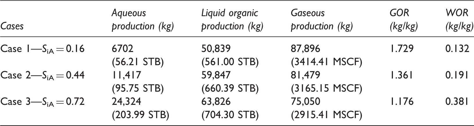
ICP: in-situ conversion process.

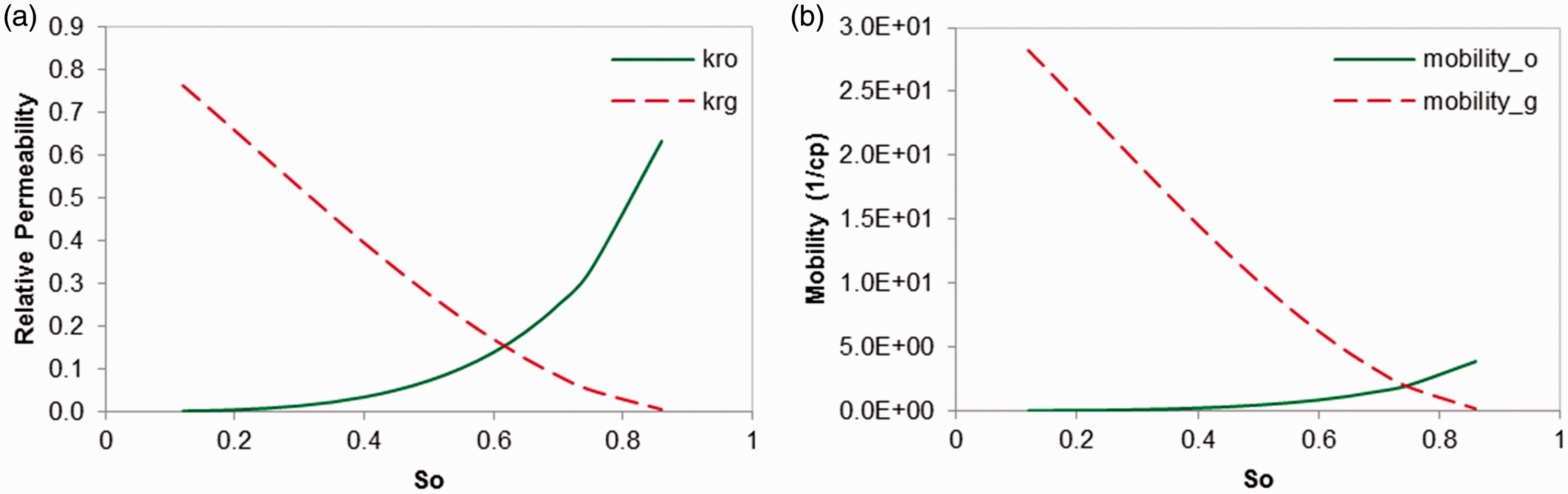
The saturation curves of fluid phases at the monitoring point (x, y) = (2.56 m, 2.56 m) are provided in Figure 14. In the fracture domain, gaseous phase replaces the liquid organic phase and aqueous phase as production proceeds, while above 60% of liquid organic phase still has remained in the matrix domain at the end of the process in each case. The curves of relative permeability from Parker’s model and the mobility of liquid organic phase and gaseous phase in the system with S_A = 10% are provided in Figure 15. Despite the higher relative permeability of liquid organic phase above S_o = 0.61, the far higher mobility of gaseous phase has caused the flow of only gaseous phase from the matrix domain to the fracture domain and the trapping of liquid organic phase in the matrix domain at the end of the process.

Figure 14.

Results of ICP cases—saturations of fluid phases in the fracture domain and matrix domain at the monitoring point (x, y) = (2.56 m, 2.56 m).

Figure 15.

Relative permeability and mobility curves of liquid organic phase and gaseous phase in the matrix domain, where S_A = 0.1.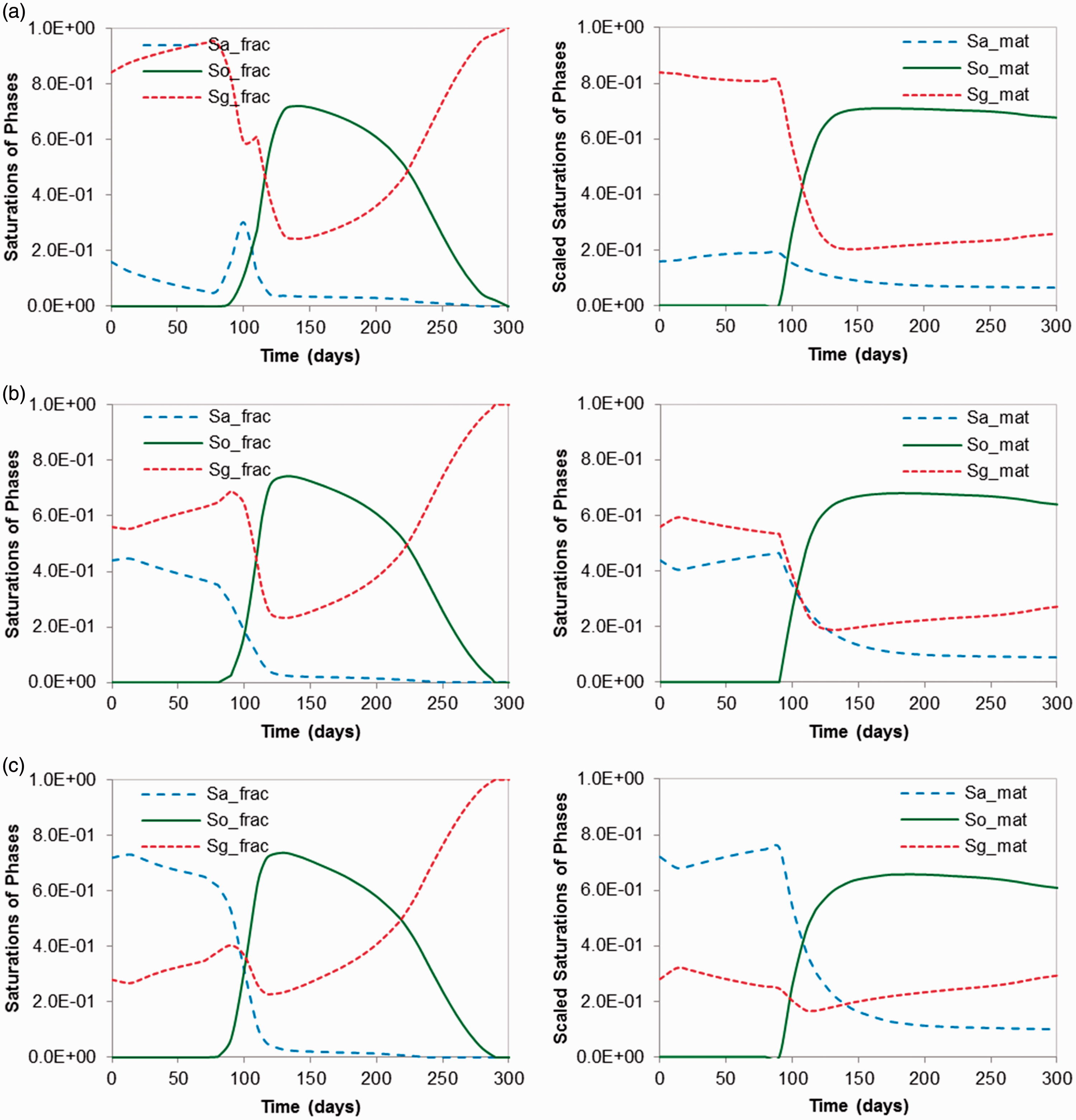

Production of components

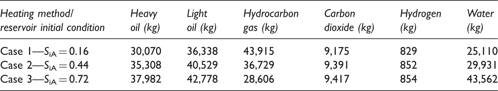
The production rates and cumulative productions of fluid components during the process are provided in Figure 16. Hydrocarbon gas, light oil, and water components have taken the highest portion of the produced fluids in the case 1, 2, and 3, respectively. The cumulative productions of the components are summarized in Table 7. Cumulative production of every component except for hydrocarbon gas increases with increasing initial saturation of aqueous phase. More carbon dioxide and hydrogen have been produced in the case with higher initial saturation of aqueous phase; they have been produced as dissolved in aqueous phase and liquid organic phase, as well as in the form of free gas. In every case, the higher cumulative production of light oil than heavy oil has been caused by the cracking reactions of heavy oil into lighter hydrocarbons, as well as by the higher mobility of light oil.

Figure 16.

Results of ICP cases—production rates and cumulative productions of components.

Table 7.

Cumulative productions of components in the ICP cases.

Heating method/ reservoir initial condition	Heavy oil (kg)	Light oil (kg)	Hydrocarbon gas (kg)	Carbon dioxide (kg)	Hydrogen (kg)	Water (kg)
Case 1—S_iA = 0.16	30,070	36,338	43,915	9,175	829	25,110
Case 2—S_iA = 0.44	35,308	40,529	36,729	9,391	852	29,931
Case 3—S_iA = 0.72	37,982	42,778	28,606	9,417	854	43,562

ICP: in-situ conversion process.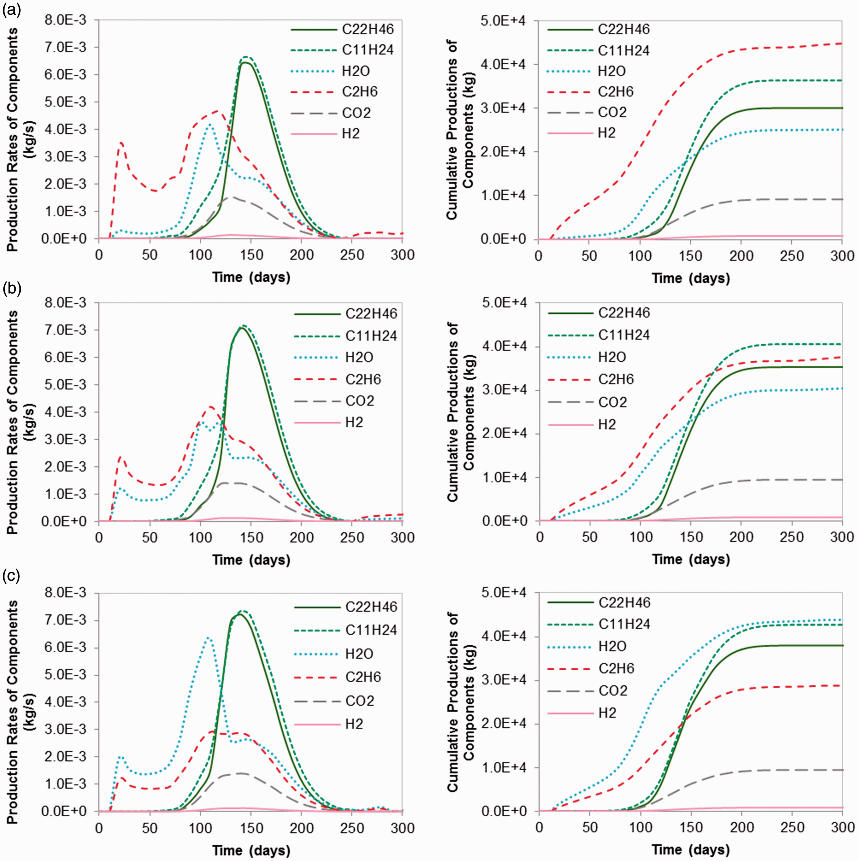

Conclusion

In this study, we have investigated the effects of initial saturations of fluid phases in the reservoir and diverse thermal methods on production behavior by conducting two sets of simulations—five-spot well pattern problems and ICP problems. From the first set of five-spot well pattern problems, we have the following conclusions.

The increase of system temperature and the decomposition of kerogen in the system have been fastest in the case of hot water injection in the aqueous phase reservoir, by the vigorous heat transfer by conduction and convection.

The final effective porosity and absolute permeability of rock matrix in each case has approached 0.2 and 3.111 md, respectively.

The case of hot water injection in the aqueous phase reservoir has showed the largest cumulative productions of hydrocarbons (heavy oil, light oil, and hydrocarbon gas) among the cases, even also has showed the largest WOR.

Enormous energy loss and huge operating cost are expected in the case of hot water injection. The envisioned work will include the analysis of energy efficiency and economic feasibility of each case.

From the second set of ICP problems, we have the following conclusions.

Even the cases have different initial saturations of fluid phases in the system, the difference of speed of kerogen decomposition is insignificant by the low initial effective porosity of the system.

The final effective porosity and absolute permeability of rock matrix in the cases have approached 0.17 and 0.642 md, respectively.

In every case, gaseous phase has showed the highest mass of cumulative production among the phases. More liquid organic phase has been produced with the higher S_iA, by the less production of gaseous phase.

At the end of the heating and production process, only gaseous phase has flowed through the fracture domain, while above 60% of liquid organic phase has been trapped in the matrix domain due to its far lower mobility than the gaseous phase.

Footnotes

Acknowledgments

The authors would like to appreciate the Crisman Institute for Petroleum Research of Texas A&M University for supporting this study.

Declaration of conflicting interests

The author(s) declared no potential conflict of interest with respect to the research, authorship, and/or publication of this article.

Funding

The author(s) disclosed receipt of the following financial support for the research, authorship, and/or publication of this article: This study was financially supported by the Crisman Institute for Petroleum Research of Texas A&M University (Crisman project number: 1.7.05b).

References

Crawford

Killen

(2010) New challenges and directions in oil shale development. In: Ogunsola

Hartstein

Ogunsola

(eds) Oil Shale: A Solution to the Liquid Fuel Dilemma, Oxford: Oxford University Press, pp. 21–60.

Dyni

(2006) Geology and resources of some world oil-shale deposits, Denver: US Department of the Interior, US Geological Survey, pp. 2005–5294.

Fan

Durlofsky

Tchelepi

(2010) Numerical simulation of the in-situ upgrading of oil shale. SPE Journal 15(2): 368–381.

Fowler

Vinegar

(2009) Oil shale ICP-Colorado field pilots. In: SPE western regional meeting, San Jose, California: 24–26 March, Society of Petroleum Engineers.

Kibodeaux KR (2014) Evolution of porosity, permeability, and fluid saturations during thermal conversion of oil shale. In: SPE annual technical conference and exhibition, Amsterdam, The Netherlands, 27–29 October, Society of Petroleum Engineers.

Knaus

Killen

Biglarbigi

(2010) An overview of oil shale resources. In: Ogunsola

Hartstein

Ogunsola

(eds) Oil Shale: A Solution to the Liquid Fuel Dilemma, Oxford: Oxford University Press, pp. 3–10.

Krauss

Mays

(2014) Modification of the Kozeny-Carman equation to quantify formation damage by fines in clean, unconsolidated porous media. SPE Reservoir Evaluation & Engineering 17(4): 466–472.

Lee K (2014) Rigorous simulation model of kerogen pyrolysis for the in-situ upgrading of oil shales. Doctoral dissertation, Texas A & M University, pp. 38–170.

Lee

Moridis

Ehlig-Economides

(2016a) Numerical simulation of diverse thermal in-situ upgrading processes for the hydrocarbon production from kerogen in oil shale reservoirs. Energy Exploration and Exploitation. (accepted 11 August 2016).

10.

Lee

Moridis

Ehlig-Economides

(2016b) A comprehensive simulation model of kerogen pyrolysis for the in-situ upgrading of oil shales. SPE Journal 21(5): 1612–1630.

11.

Nimblett J and Ruppel C (2003) Permeability evolution during the formation of gas hydrates in marine sediments. Journal of Geophysical Research: Solid Earth 108(B9): 2420.

12.

Pruess

(1985) A practical method for modeling fluid and heat flow in fractured porous media. Society of Petroleum Engineers Journal 25(1): 14–26.

13.

Shen C (2009) Reservoir simulation study of an in-situ conversion pilot of Green-River oil shale. In: SPE rocky mountain petroleum technology conference, Denver, Colorado, 14–16 April. Society of Petroleum Engineers.

14.

Symington W (2006) ExxonMobil’s Electrofrac process for in situ oil shale conversion. In: 26th oil shale symposium, Golden Colorado, Colorado, 16–20 October, Colorado School of Mines.

15.

Thoram S and Ehlig-Economides CA (2011) Heat transfer applications for the stimulated reservoir volume (SRV). In: SPE annual technical conference and exhibition, Denver, Colorado, 30 October–2 November, Society of Petroleum Engineers.

16.

Vinegar H (2006) Shell’s in-situ conversion process. In: 26th oil shale symposium, Golden Colorado, Colorado, 16–20 October, Colorado School of Mines.

17.

Wellington SL, Berchenko IE, De Rouffignac EP, et al. (2005) In situ thermal processing of an oil shale formation to produce a condensate. Google Patents (US 6880633 B2).

18.

Youtsos

Mastorakos

Cant

(2013) Numerical simulation of thermal and reaction fronts for oil shale upgrading. Chemical Engineering Science 94: 200–213.

Compositional simulation of hydrocarbon recovery from oil shale reservoirs with diverse initial saturations of fluid phases by various thermal processes

Abstract

Keywords

Introduction

Simulation model description

Simulation of five-spot well pattern problems

Simulation model and initial reservoir properties

Simulation results and discussion

System behavior

Kerogen mass in place and productions of phases

Productions of components

Simulation of ICP

Simulation model and initial reservoir properties

Simulation results and discussion

System behavior

Production of phases

Production of components

Conclusion

Footnotes

Acknowledgments

Declaration of conflicting interests

Funding

References