
Abstract
Climate change is one of the greatest challenges the building industry faces. Engineers and architects require representative future weather data if they would like to see how their buildings and designs will fare under a changing climate. The most common method used to create future weather involves manipulating observations commonly known as morphing, but the most used algorithms can create implausible weather conditions due to their unbounded nature. Here, bounded morphing algorithms will be described and their effectiveness proved mathematically. The improved bounded method applies two additional conditions on the morphed distribution to the maximum and minimum values, in addition to the mean values. The benefits over the standard approach will also be illustrated considering the changes in the distribution of temperature and solar irradiation due to climate change. The improved algorithms outperform the standard morphing procedures in terms of preserving the underlying climate signal while not creating unrealistic or implausible weather conditions. This method should give engineers confidence that the generated future weather series are more robust and representative of potential future weather.
Introduction
Hourly weather data files or weather years are an important resource for building simulation studies. These weather files mostly take the form of typical weather years of a particular location and are created from historic observations.1,2 There are several approaches that have been adopted for the generation of typical weather files such as the Test Reference Year (TRY), 3 Typical Mereological Year (TMY) 4 or International Weather for Energy Calculation (IWEC). 5 The process for creating the files is similar with weather variables in a given month ranked to determine the most average, from which the most average months are assembled to create a composite average year. Such weather years can form the industry-standard and their use can be a requirement by building regulations and other codes and standards. For example, in the UK, the Chartered Institution of Building Services Engineers (CIBSE) provides a set of TRY weather years which since 2006 have been made available for 14 site locations.1,3 Additionally, in some countries warm weather data sequences are used for the purpose of overheating risk analysis and cooling system sizing, for example in the UK, the CIBSE Design Summer Years.3,6
In all these cases, the weather years are based on historical observed data. Climate change presents the likelihood that the historic climate we have experienced in the past is unlikely to be representative of the weather conditions that will be experienced in the future over the next few decades. 7 In recent years, the world has experienced unprecedented extreme events. The European heat wave of 2019 has been found to be 10 times more likely due to climate change. 8 This single event broke several records at single locations and for example exceeding the highest temperature recorded in France by 2°C and caused excess mortality in the thousands.9,10
Such heat events though are expected to become more common. 7 The warming will largely be driven by anthropogenic emissions, a warmer atmosphere with modifications due to aspects such as the position of the Jet streams. Whilst these local effects are uncertain, studies have demonstrated that Europe is warming faster than the rest of the northern midlatitudes over the past 42 years due to more persistent double jets over Europe. 9 Across the world it is expected that warmer temperatures will be compounded with more frequent heatwaves and drought. 10 It has long been suggested that using historic observations for building design could be inappropriate considering the potential impact of climate change,11,12 and the speed and unprecedented nature of recently observed extreme weather events further puts their use into question.
In recognition of the need to take account of future climate changes in building design, CIBSE introduced in 2009 a set of TRY and DSY weather years reflective of possible future climates based on the UK government’s UKCIP02 climate change scenarios for the United Kingdom. These weather years were called the CIBSE Future Weather Years. The methodology used to produce the CIBSE Future Weather Years is described in CIBSE TM48. 13 The methodology was based on a method to apply the climate change projections to the existing weather file which was called ‘morphing’. 14 The morphing method consists of adjusting an observed weather year using a set of mathematical operations that result in a new weather year that has new average monthly climate conditions consistent with the climate change projections but retains the hour-to-hour variability of the observed weather timeseries. The morphing method is one of several ‘downscaling’ methods through which the coarse spatial and temporal scale information from climate models can be incorporated to produce the site-specific hourly weather data required for building simulation. 15
While the use of future weather data within building simulation is now very much commonplace within research and industry, nearly all studies use Belcher et al.’s morphing method. Even a recent open access tool uses the morphing methodology exactly as described by Belcher et al. 16 However, there are clear compromises in the use of this method. For example, as discussed by Belcher et al., not all characteristics of the predicted change in temperature could be preserved within the transformed data. In recognition of the limitations of the Belcher et al. algorithms, a revised set of algorithms were developed by researchers at Arup for the CIBSE TM49 project, which developed new Design Summer Years for London. 17 These algorithms were also used in the production of the 2016-issue CIBSE weather years 18 and have been used in the Arup proprietary tool WeatherShiftTM. 19 While Dickinson and Brannon briefly introduced the concept of a bounded transformation, 19 to date there has been no published proof that such algorithms are suitable or how they improve on the original morphology methodology.
In this work we will first go through the original morphing procedure in detail to demonstrate its limitations with respect to the adjustment of temperature data. We will then describe the revised morphing algorithms which we term a Weighted Stretch and a Bounded Temperature Weighted Stretch. Most of the impacts on the transformed weather series are self-evident from the mathematical formulation of the approach taken, but in the results, we will show the key differences between the revised and the Belcher et al. morphing algorithms on the transformed weather files including the impacts on the outputs from building simulation.
Original morphing algorithms
The creation of a future weather file using a morphing method starts with a timeseries of observations of a weather variable,
A simple shift can be defined by,

A simple stretch is defined as,

A shift and stretch is defined as a combination of a simple shift and a simple stretch and is defined by

UKCP18 probabilistic change factors and units.
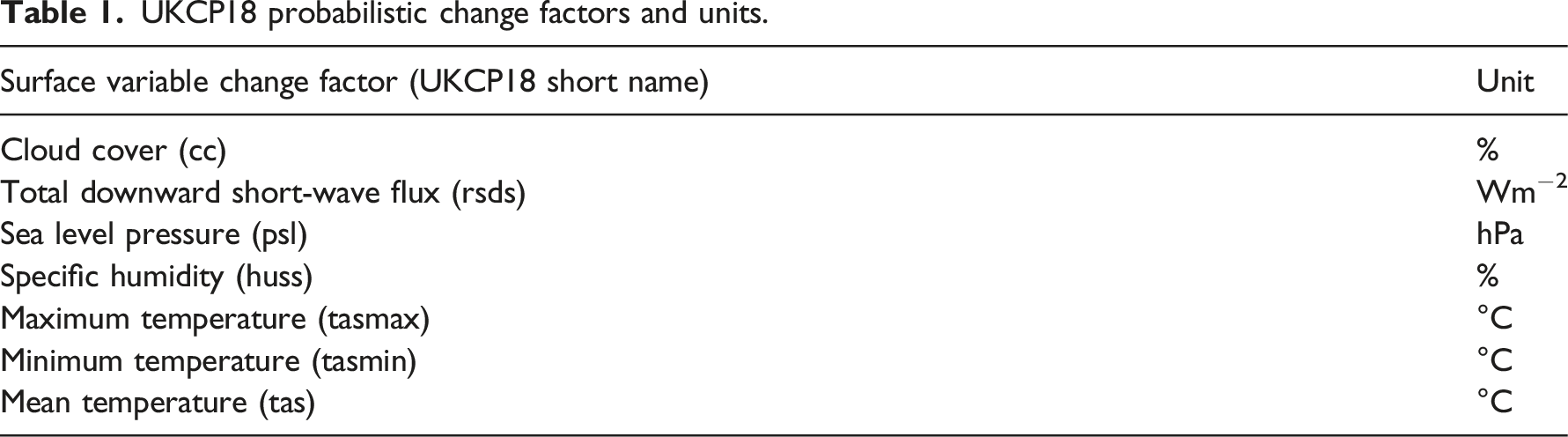
Cloud cover is measured in Oktas, but the change factor is a percentage change. The first step is to convert the percentage change to an absolute value whereby equation (1) could be applied.
Solar radiation has a clear diurnal cycle, and any change must preserve this distribution. The change factor though is given as an absolute change. The absolute change can be converted to a fractional change by normalising the change to the observed baseline ie
The sea level pressure can be calculated by taking the observed atmospheric pressure and applying the equation (1) using the absolute change specified in the projections.
Specific humidity is not observed but can be calculated from temperature, air pressure and relative humidity which are all measured. The specific humidity is given as a percentage change so the change factor can be derived from
Dry bulb temperature (dbt) has three change factors associated. Namely the change in the mean, daily maximum and daily minimum of which all three are used to derive the morphed time series. The scaling factor is given by: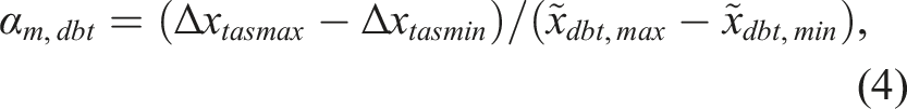
The application of the morphing algorithms is relatively straight forward in each case. However, there are some clear limitations with this method. 1. Morphing the dry bulb temperature preserves the change in the mean temperature and the change in average diurnal temperature range given by the three change factors but not the projected daily average maximum temperature and daily average minimum temperature independently. It can be verified that:

Hence only one of the change factors is conserved in the new time series. 2. For variables such as cloud cover there is a physical limit which the transformed time series can not go beyond. In this case no lower than a clear sky (0 Oktas) and no higher than full sky cover (8 Oktas). The case of a negative (positive) change factor means a reduction (an increase) in all cloud cover measurements but any observation of 0 (8) Oktas would remain unchanged. Hence the morphed time series would not preserve the climate change anomaly.
Given the shortcomings of the morphing method there was a need to propose a new methodology which maintains the underlying climate projections.
Bounded weighted stretch morphing algorithms
In this section the details of the revised algorithms that were used for CIBSE TM49 are described (Hacker, 2014, pers. comm.) as well as the required mathematical proofs.
The problems identified in the previous section can be characterised as the need to preserve the physical and natural limits of some weather variables or there is a need to preserve additional features of the distribution of the transformed time series such as the change in the average daily maximum temperature. This imposes an upper and lower bound to the transformation which means the morphing procedure must preserve these conditions. For a normalised input bounded between 0 and 1: 1. If 2. If 3.
where
A transfer function (g) which can be applied is symmetric and takes the form:
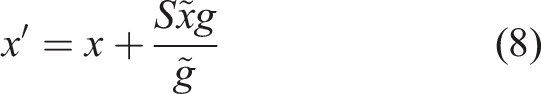
For temperature, the scaling factor would need to include information about the change in the average daily maximum temperature, and the change in the average minimum temperature as well as the change in mean temperature. The input daily temperature time series (T) should be normalised between 0 and 1. This can be achieved by applying: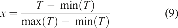


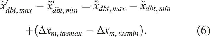
To get the transformed temperature series, the output from equation (8) must be combined with equations (10) and (11) to maintain the physical change in the daily maximum and minimum temperatures: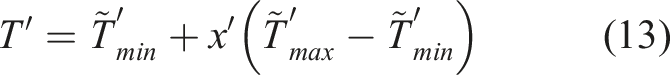
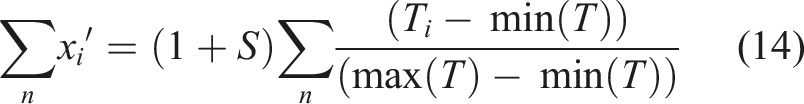
Likewise, taking the sum of equation (13) over all possible values gives the equation: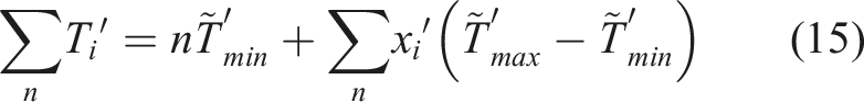
Since 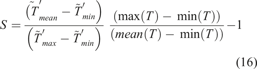
It can be shown that taking the average value of equation (13) and substituting in the values for
Application of morphing algorithms to real weather data
The purpose of using a morphing algorithm is to generate future weather data which is representative of the projections of climate change. In this work the exact nature of the climate change projections is not that important since here it is only necessary to prove the effectiveness of the bounded weighted stretch algorithm compared to the original method. The baseline for UKCP18’s probabilistic projections are from 1961–1990, 1981–2000 and 1981–2010. A climate norm is usually considered as a 30-year period therefore the baseline of the projections will be from the period 1981–2010. All climate change projections from the RCP8.5 scenario for the period 2071–2100 (or 2080 s) so the widest range of climate change projections (or change factors) are used in the analysis. At each period, 3000 samples, or probabilistic projections are available, and all 3000 will be tested here. The projections are shown in Figure 1 for February and Figure 2 for August. The change factors for mean temperature ( UKCP18 change factors for the 2080s in February. UKCP18 change factors for the 2080s in August.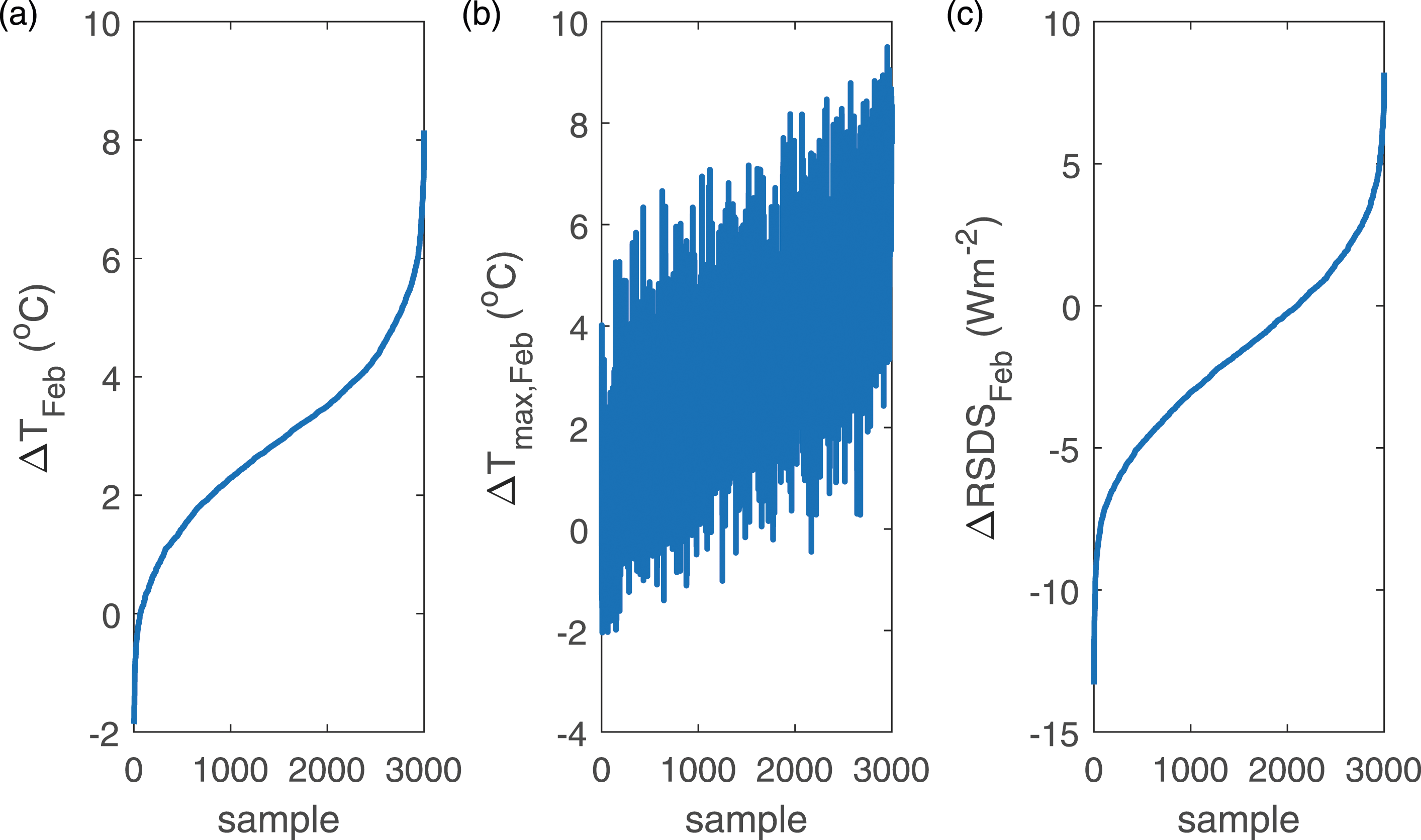
Weather observations from London Heathrow (Latitude 51.479 N, Longitude −0.449 E, WMO station ID:03772) will be considered as this will contain a range of very hot and cold weather over the time series whilst the observations from Heathrow at this location are mostly complete for example only 0.12% of the temperature data is missing. 20 Missing data will be interpolated using standard methods. 1 Building performance analysis is usually evaluated using a representative year. For heating energy, a TRY would be used so a TRY will be created using the same 1981–2010 baseline and methods used to create the current UK industry standard TRYs 1 to which the morphing algorithms will then be applied. Like most locations around the world, solar radiation is not recorded at this weather station. While measurements from satellites are available from 2004, this would only give 7 years of data. For consistency solar radiation will be recreated using the Meteorological Radiation Model. 21
The morphing algorithms will be applied following the original procedures and the bounded weighted stretch algorithms as appropriate. Here we are interested in the key differences between the morphing algorithms beyond the application of the change factors since the suitability has already been shown. From the deductions in section 4 the change factors will be realized in the morphed weather series using the bounded weighted stretch algorithm. This is also mostly true for the original algorithms. For example, when using Belcher’s method to morph the temperature, the mean of the future weather series will be equal to the mean of the original series plus the change factor. However, i.e. not true for the change in daily maximum and daily minimum temperatures. Also, the impact on the absolute maximum and minimum temperature is not certain given it is also a function of the change in mean temperature. The comparisons will take the form: 1. The difference between the expected change factor and the achieved change factor for the maximum daily and minimum daily temperature using the combined simple stretch and shift for all 3000 UKCP18 samples. 2. The difference between the monthly absolute maximum and minimum temperatures using the bounded temperature weighted stretch and the combined simple stretch and shift for all 3000 UKCP18 samples. 3. The change in the global radiation using the bounded weighted stretch and the simple stretch algorithms.
The external temperature is the key weather variable for considering how much heating and cooling energy may be required to maintain thermal comfort within a building. The heating and cooling degree days are a simple measure of how hot or cold a year and are highly correlated to the expected heating and cooling loads. The degree days are computed from counting the hours where a threshold has been exceeded and then dividing by 24 to convert it to hours. Heating degree days will be calculated with a threshold of 10°C and 18.3°C and the cooling degree days with a threshold of 23.3°C and 26.7°C corresponding with those as presented in ASHRAE handbook fundamentals. 22 Solar radiation is often a key factor in determining cooling loads hence it is also included in the comparison.
In all cases only individual months and weather variables will be considered as it is beyond the scope of this paper to consider the impact of the selection of climate change scenarios and joint probabilities of coincident weather variables.
Finally, the impact of the two algorithms across all weather variables will be demonstrated through building simulation using all 3000 samples from UKCP18 using EnergyPlus. The building considered here is a large two-story house constantly used by four people with a total conditioned area of 164 m2 sat mostly above a 130 m2 unconditioned garage. It is orientated north-south with a rectangular form. The house is intended to represent a high-performance building with a current heating requirement of 15 kWhm−2 with a thermostat of 20°C The house is simplified with all rooms combined into a single zone. The U-values of the wall, roof and floor of the conditioned zones are equal to 0.12 Wm−2K−1, 0.21 Wm−2K−1, 0.20 Wm−2K−1 respectively. There are 54 m2 of windows, 50% are orientated to the South and 40% north, with a U-value of 1.35 Wm−2K−1. The infiltration is set at 0.1 ACH. For simplicity the space is maintained at a constant 20°C all year round using an ideal loads system with the differences in heating and cooling energy (as a proxy for thermal discomfort) explaining the differences in the different morphing approaches.
Results and discussion
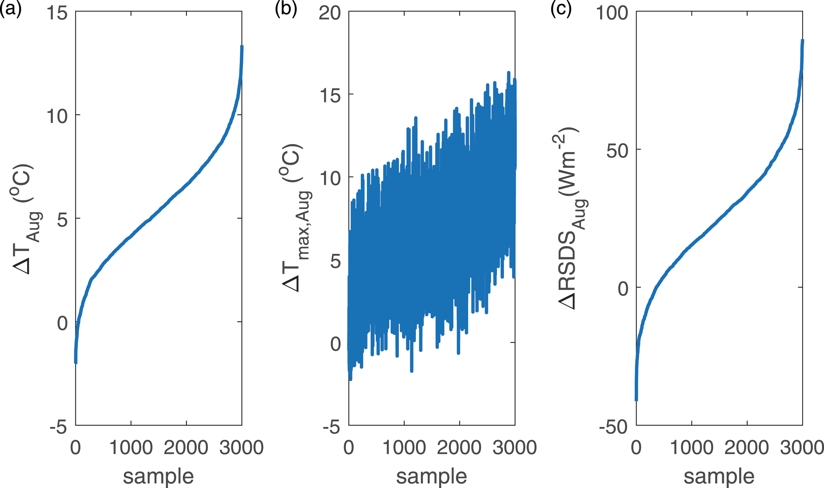
Figure 3 shows the actual change factor from applying the Belcher et al. algorithm in comparison to the expected change factor as obtained from UKCP18. There is no clear trend with the change factors scattered around the expected change factor (marked by the solid line). Only 10% are within 0.2°C of the expected value. The average difference is around 1.1°C for February and 1.7°C for August. Figure 4 shows the same comparison using the BTWS algorithm. 50% of all points sit on the expected line and in total 70% of the values are within 0.2°C. The average difference is around 0.4°C for February and 0.3°C for August. Small deviations from the expected values are where the application of the change factors on a small number of day results in an unphysical relationship where the morphed minimum (maximum) temperature is larger (smaller) than the morphed mean temperature. In these cases, only the change in the mean on that day is applied which in turn affects the overall distribution that month. Larger differences are where the change factors mostly result in unphysical changes across the month. A comparison of the expected change factor (UKCP18 projection) against the actual change factor using the Belcher algorithm for average daily maximum and average daily minimum temperature for February and August. The straight lines are what would be expected with a perfect fit. A comparison of the expected change factor (UKCP18 projection) against the actual change factor from using the BTWS algorithm for average daily maximum and average daily minimum temperature for February and August. The straight lines are what would be expected with a perfect fit.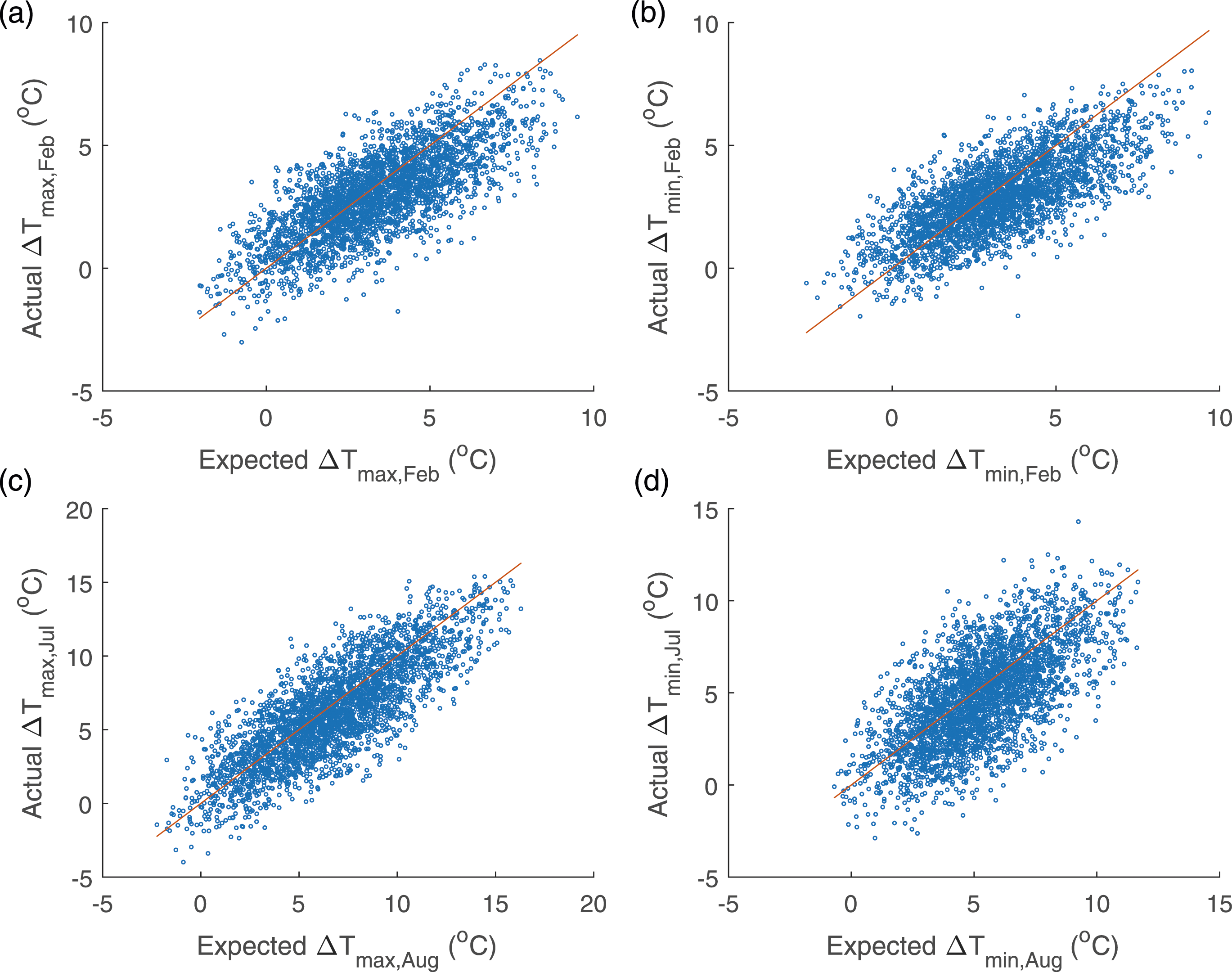
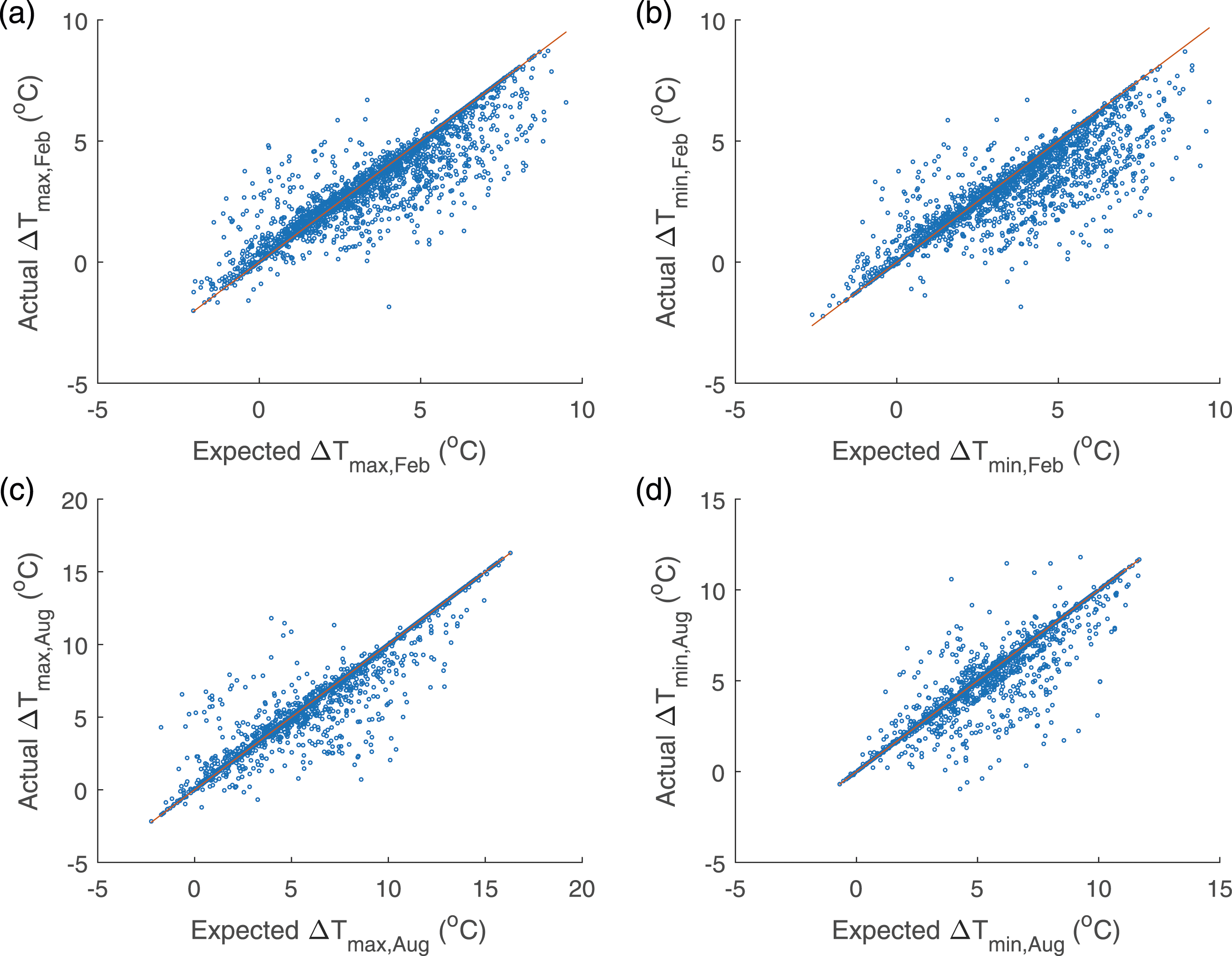
Figure 5 shows the heating degree days in February and the cooling degree days in August against the difference in the projected change in daily maximum and minimum temperatures for all 3000 climate projections from the chosen climate scenario. If the two morphing algorithms give a similar temperature distribution, then the outcome will be a small cluster around 0. Where the change in maximum temperature is greater than the expected change in minimum temperature, the Belcher algorithm gives more heating degree days and more cooling degree days. The exception is for a base temperature of 18.3°C where both algorithms give a similar number of heating degree days where the change in minimum temperature is larger than the change in maximum temperature. Comparison of (a) heating degree days at 10°C in February and (b) heating degree days at 18.3°C (c) cooling degree days at 23.3°C in August and (d) cooling degree days at 26.6°C in August against the difference between the projected change in maximum and minimum temperature in the same month using either the BTWS algorithm and Belcher algorithms.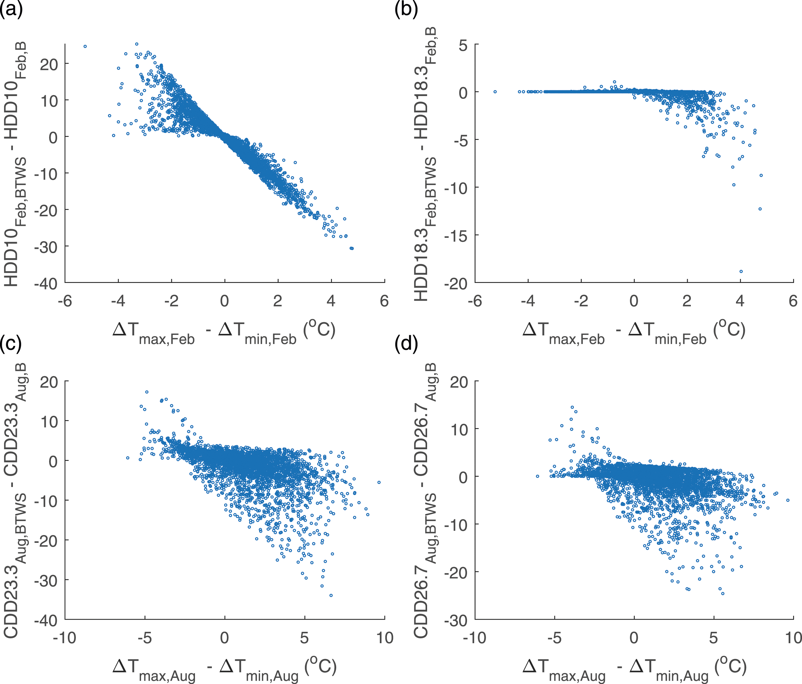
Across all samples, the average difference between the two algorithms for heating degree days is 1.2°Days with a base temperature of 10°C and 0.2°Days with a base temperature of 18.3°C. For cooling degree days, the average difference is 2.1°Days with a base temperature of 23.3°C and 1.3°Days for a base temperature of 26.6°C. The standard deviation is much larger at around 7°Days for all except for heating degree days with a base temperature of 18.3°C where the standard deviation of the difference is 0.8°Days showing the variability and dependence on the applied change factors.
The differences found in Figure 5 are simply a result of the application of the two transformations. For example, Figure 6(a) shows the morphed February temperature considering Example morphed temperatures using the Belcher and BTWS algorithms in (a) February with 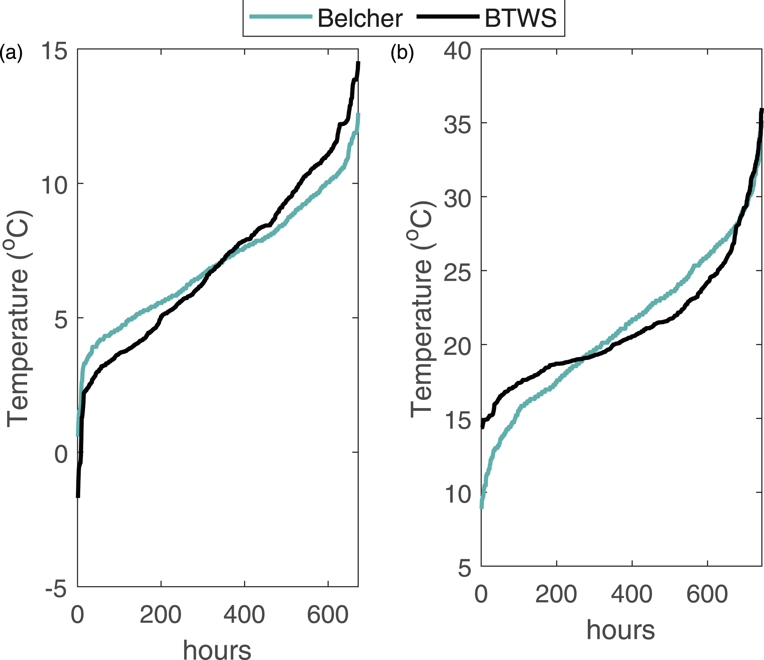
In Figure 6(b) the Belcher algorithm under predicts the change in minimum and maximum temperatures by a larger margin (
The biggest difference between the two algorithms is the ability to preserve the change in the daily average minimum temperatures and daily average maximum temperature but as found in Figure 3, that is rarely the case for the Belcher algorithm.
As expected, morphing the solar radiation results in an identical change in the amount of solar radiation for both algorithms. i.e. if the change factor suggests a five Wm−2 then both algorithms result in an increase of five Wm−2. Because the change in the mean is also preserved, the total solar radiation is also identical. Figure 7 shows the maximum monthly solar radiation using both morphing algorithms. The peak in the solar radiation for the BWS algorithm is identical to the original weather file while for the Belcher, simply reflects the distribution of the change factors. Most change factors suggest the solar radiation will increase in the summer months, but the picture is more mixed in the winter. In extreme cases, the maximum global horizontal radiation is greater than 90% of extra-terrestrial solar radiation for that hour (June and July). This implies that the application of the Belcher algorithm alone is not appropriate and further post processing would be required to ensure the output is physically consistent with what is possible. Maximum monthly global horizontal radiation using the Belcher and BWS algorithms.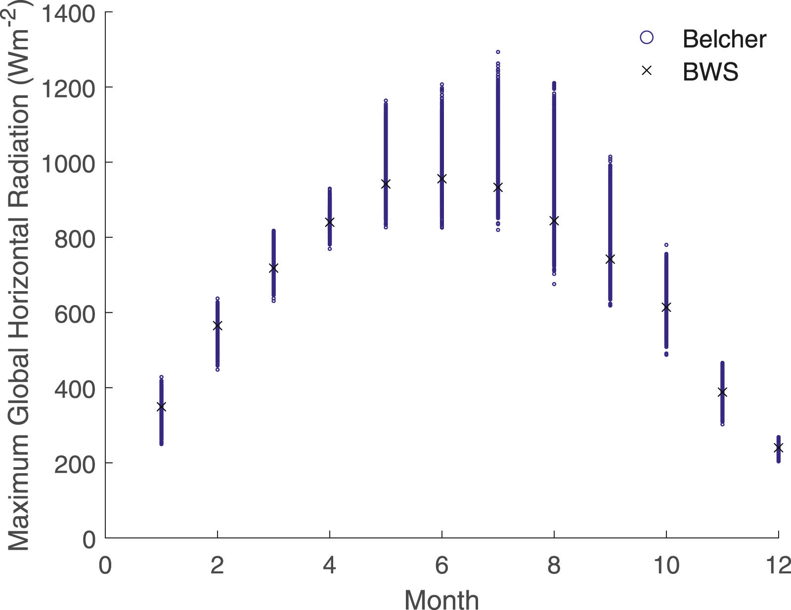
Figure 8 shows a comparison of the Belcher and BWS algorithms applied to August with a change factor of −40% (8a) and +90% (8b) which represents the full range of change found in the UKCP18 projections for the month of August. The WS algorithm maintains the peak from the original weather file in both cases whereas the Belcher algorithm morphs all values by the same percentage. Where the change factor is positive (8b) less sunny days are in effect made sunnier. If the change factor is negative, less sunny days are made less sunny, but the peak remains – the day with the greatest sunshine will still have a large solar radiation value. The largest increases and decreases are found around the mean which is a direct result of the transfer function used as expected. This would mean that on cloudless days in the summer, maximum solar radiation would be expected regardless of the change factor. Simply the weather data within the file should be physically consistent. In the case of a negative change factor this would not be the case for the Belcher algorithm and in the case a positive change factor, the peak would be much larger than expected and larger than is physically possible. A comparison of the distribution of the WS and Belcher algorithms applied to global horizontal radiation with a change factor of (a) −40% and (b) +90%. All zeros have been excluded.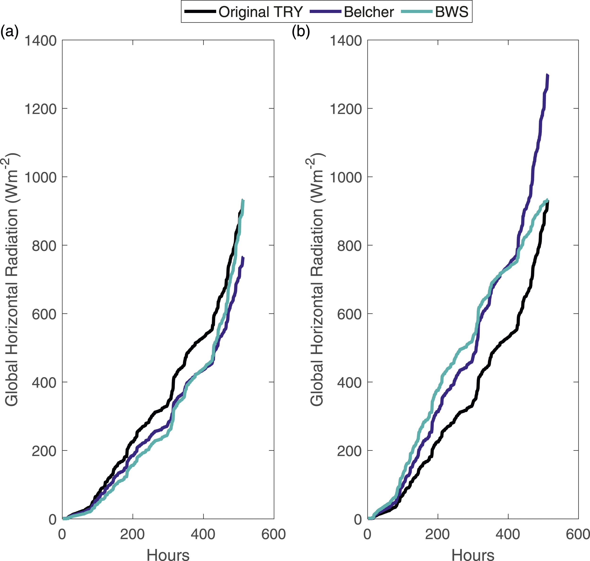
The changes in cooling degree days and solar radiation suggest that there would be an impact on building design and potential adaptations to deal with the impacts of climate change, but the combined impact of these variables has not been tested. Here all 3000 samples are used with both algorithms to compare the differences in heating and cooling energy. In the next two figures, all results will be displayed as the result using the weighted stretch algorithms subtracted from the result of using the Belcher algorithm. A positive value therefore suggests the Belcher algorithm predicts a larger total. Figure 9 shows the difference between the simulated total heating energy (9a) and the simulated total cooling energy (9b) using the Belcher and various weighted stretch algorithms. The mean difference in total heating energy is −112 kWh while the mean difference in cooling energy is 1310 kWh. The Blecher algorithm predicts heating energy will change between 95% reduction to 26% increase whereas the weighted stretch algorithms predict between 95% reduction and 32% increase across all samples. For cooling the Belcher algorithm predicts between 8% reduction to a 275% increase compared to between an 8% reduction and 253% increase for the weighted stretch algorithm. In the case of heating, there can be larger differences where increased temperature differences and reduced solar gains for example can combine to increase the temperature difference and thus heating energy requirement. But this can go both ways, with significant differences between the algorithms at the extremes. For cooling, the weighted stretch algorithm consistently predicts a reduced cooling demand suggesting that the Belcher algorithm predicts higher solar gains and/or higher temperatures leading to higher indoor temperatures. A comparison of the distribution of (a) the yearly total heating energy (b) the yearly total cooling energy from using the Belcher and WS algorithms on a complete weather file using building performance simulation. The data is presented as the result from WS algorithms subtracted from the Belcher algorithm for all climate change anomalies from UKCP18. A positive number means the energy derived from the Belcher algorithm results in a larger energy requirement.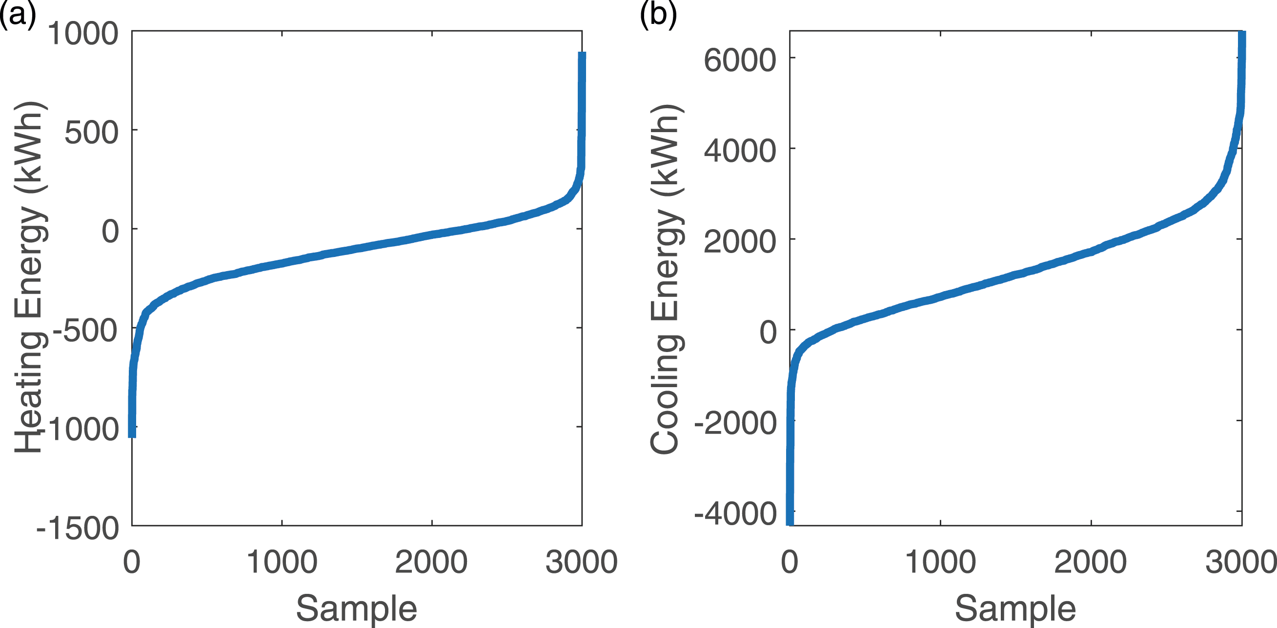
Finally Figure 10 shows the difference in the peak hourly heating energy (10a) for December, January and February and peak cooling energy (10b) for June, July and August. This shows the impact of different weather patterns in each month combined with the application of different climate change anomalies. The same patterns from Figure 9 are repeated here with peak cooling energy typically higher with a mean of 0.5 kWh larger and the maximum difference up to 2.7 kWh. The peak heating energy can be as large as 1.2 kWh, but the average is around 0. A comparison of the distribution of (a) the peak heating energy in the winter months and (b) the peak cooling energy in the summer months from using the Belcher and WS algorithms on a complete weather file using building performance simulation. The data is presented as the result from WS algorithms subtracted from the Belcher algorithm for all climate change anomalies from UKCP18. A positive number means the energy derived from the Belcher algorithm is results in a larger peak load.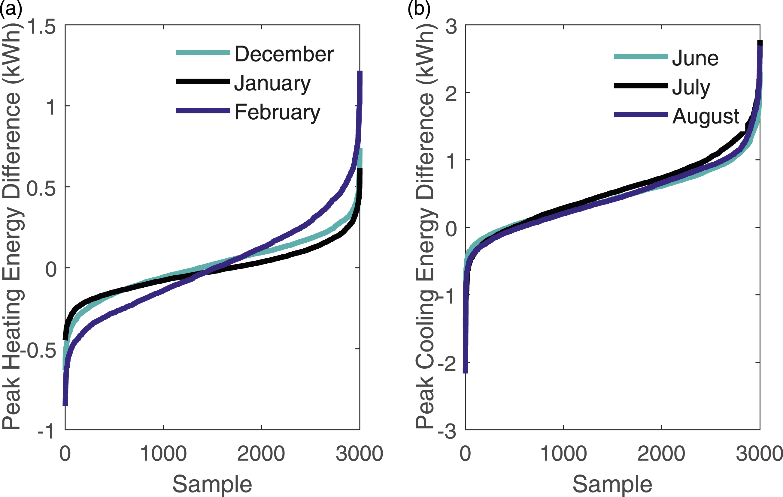
This suggests that while changes in the total energy clearly depend on the month and the climate change anomalies applied, the choice of algorithm would impact the ability to meet a benchmark energy performance such as meeting the Passivhaus requirement for total space conditioning as well as impacting on plant sizing.
Conclusions
In this work a set of revised morphing algorithms have been described and these have been shown to improve upon the shortcomings of the algorithms proposed by Belcher et al. Namely, (1) the ability to preserve changes in the mean, daily average maximum and daily average minimum temperatures and (2) the ability to preserve physical limits in the transformed weather series. These revised algorithms are (1) A weighted stretch which can be applied to any weather variable where only one change factor is known and (2) A bounded temperature weighted stretch which is applied to the dry bulb temperature where three change factors are typically available to describe the changes due to climate change. The revised algorithms have been shown to outperform the original methods in terms of maintaining the temperature change factors in the morphed weather data. When the original morphing method is applied to solar radiation this could create a peak value that was unrealistic in terms of consistency with the underlying weather – much less than expected or much greater than expected on a cloudless sky – which is impossible with the revised method.
While the revised method leads to changes in the resultant weather variables, it is also found that using the revised morphing algorithms results in changes in the indoor environment when used to create a future weather file combined with building performance simulation and thus different design decision would be made. The simulations carried out here suggests that the new weighted stretch algorithms would result in reduced heating energy on average for the same climate change prediction/climate change anomalies as well as reduced cooling energy including the reduction in peak loads. This means that the revised algorithms would mean a direct impact on building design around provision of building services and the ability to maintain thermal comfort.
The selection of transfer function is pragmatic in ensuring that the transformed weather data was symmetric about the mean value. But it is not clear from this work whether this is the most appropriate choice. When morphing the temperature, the algorithm is adapted to become asymmetric for circumstances where the transformation results in values that go outside the physical bounds (where
Footnotes
Authors’ note
Ruth Shilston is now at Mott MacDonald
Declaration of conflicting interests
The author(s) declared no potential conflicts of interest with respect to the research, authorship, and/or publication of this article.
Funding
The author(s) disclosed receipt of the following financial support for the research, authorship, and/or publication of this article: This work was supported by the Innovate UK.