
Abstract
Weather files are fundamental for building performance applications such as estimating energy demand or predicting the risk of thermal discomfort. Often such weather files are based on specific locations with limited guidance to which file to use which can lead to non-representative climate conditions for a specific building and potentially under or over engineering of systems. Recently, a new approach to generating representative weather files for building performance using climate zones has been proposed. This work presents a comparative analysis of the two approaches. Results from examining the external climate and an example building simulation reveal substantial differences: heating degree days vary by up to 931° days, cooling degree days by up to 500° days, heating energy demand differs by as much as 60%, and overheating exposure in the bedroom exceeds 26°C for up to 45 h more. Overall, we find significant variations in heating and cooling loads can be expected if unrepresentative climate data is used highlighting the importance of selecting appropriate weather data for building performance simulation. The use of zone-based files provides a more nuanced understanding of climate conditions, improving the reliability of building performance assessments and compliance with overheating standards.
Practical application
Weather files are fundamental for building performance analysis and supporting design decisions including the prediction of the risk of thermal discomfort. There is a need for these weather files to be kept up to date following the continual warming of the environment to ensure that the performance analysis represents external conditions and ensuring the analysis is fit for purpose. A significant limitation of the current approach is the uncertainty of which weather file should be used for any given location particularly in locations such as the UK. This work provides a framework for the development of climate-zones and representative weather files suitable for supporting the benchmarking of building performance across the climate zone removing ambiguity within the industry for the appropriate selection of weather data.
Keywords
Introduction
Weather files are fundamental to building performance analysis. They provide critical climatic data that influence design decisions related to energy performance, thermal comfort, daylighting, and overall building efficiency.1–5 Accurate and representative weather data allows designers to evaluate performance of buildings under various climatic conditions and optimise building design. 6 Moreover, weather files are essential in assessing the thermal behaviour of buildings. 7
Standard weather files, such as Test Reference Years (TRY) and Typical Meteorological Years, are commonly employed to represent average weather conditions8,9 and are typically used to estimate expected energy usage. 10 As the frequency and intensity of extreme weather events rise due to climate change, it becomes critical to incorporate extreme weather data into building performance evaluation, since extreme weather events can have a profound impact on a building’s energy consumption, structural integrity, and thermal comfort. Moreover, Jentsch et al. highlight that buildings designed using only historical average data are at risk of underperforming when faced with the extremes of heat. 11 It is crucial to embed the latest trend of climate change into standard weather files to ensure that buildings designed at the current date are future-proof. Thus, the development of representative extreme weather files, specifically designed to model these tail weather conditions, is crucial for designing resilient, adaptable buildings in conjunction with an idea of the general performance as can be modelled with the typical weather file.
In the UK both TRYs and probabilistic Design Summer Years (DSYs) are used for compliance within the building regulations. Specifically, TRYs are used for Part L: conservation of fuel and power12,13 while DSYs underpin part O: Overheating.14–16 However, there are two key issues with the use of these files: (1) The UK industry standard files are out of date: based on a baseline from 1984 to 2013. There has been further warming and multiple historic weather records broken across the country including the hottest temperatures. (2) Locations are fixed near urban centres, but these are not well distributed across the country. Guidance states that the most representative climate should be selected, but for many this will be hard to justify, and the most likely situation is to use the weather file nearest to the site location.
No matter how accurate building performance simulation tools are, they will only yield reliable outcomes if the weather data used for modelling accurately reflects the conditions a building will encounter throughout its lifespan. Inaccurate or flawed weather data will lead to unreliable results, which at best may be imprecise, and at worst, could be significantly misleading. Typically, weather files are constructed from historic observation at sites, normally at airports and similar, located next to urban areas.17,18 It is then the role of the user to determine which weather file is most appropriate for their building. In the UK for example, previous iterations of weather files have produced 16 sites (three for London) for use with building regulations, 19 but without further guidance a typical user would use the closest file which can have significantly different weather to where the building is located. 20
Geographical proximity does not always entail climate similarity. To enable the creation of accurate weather files which are representative of local climate, it is critical to develop a profound understanding of geographical patterns of the climate. Climate zones can then be established to amalgamate regions with a similar climate while distinguishing those with significant variations. The conventional Köppen-Geiger climate classification system, 21 which divides climates into five main climate groups and 30 sub-groups based on seasonal precipitation and temperature patterns, yields very large climate zones, not able to capture local variations. While the classification system has been updated by different groups including the impacts of climate change or the incorporation of higher resolution climate data,22,23 many countries such as the UK are split into one or two climate zones and is therefore, not suitable for applications where high resolution and granularity of climate patterns needs to be distinguished, such as weather file creation for building performance analysis. To overcome the limitations of the conventional zoning method, a hierarchical clustering method was developed and a total of 28 climate zones were created using the UK Climate Projections 2018 in our previous study. 24 To the best of our knowledge, it is the first study on dividing the UK into granular climate zones to represent local climate variations and enable more accurate creation of weather files. In contrast, none of the previous concepts of zones in building performance evaluation in the UK is based on climate.
In this work we will develop up to date weather files which cover the UK with weather files suitable for benchmarking building performance which for the first time removes the ambiguity of which file should be used for a specific site location. This will be driven by climate analysis which builds on previous work that has already defined appropriate climate zones. We will refer to these as the zone-based weather files compare the developed zone-based TRY and DSY weather files with industry standard weather files, updated to the same baseline. It is vital to know the key differences between weather files based at the UK standard locations and new zone-based files from the perspective of the external climate and how it may influence building design and then whether this reflects a change in performance through building simulation so both with will be investigated. These steps will be explained in more detail through the paper.
Methodology
Data availability is fundamental to developing weather files. As per previous studies, 17 the availability of observations is limited by the network of weather stations. Whilst there are many weather stations in the UK, most do not collect appropriate hourly weather data for the modelling of buildings via building performance simulation software. Here we restrict observations to those from the land surface synoptic observations. These mostly measure dry bulb, wet bulb and dew point temperature, cloud cover, surface pressure, wind speed and wind direction on an hourly resolution. There are over 400 weather stations which have collected this data with some stations in operation since 1949 until the present day. However, some of these stations have only collected data for a short amount of time (e.g., 1 year) or have data with a resolution of less than an hour. Additionally, there are very few stations with no gaps in the observation record.
Gaps in the data will be filled using linear interpolation for weather variables such as wind direction and wind speed. Gaps in air pressure will be filled using a spline interpolation. Gaps in temperature will be filled following a two-step process. First, the daily minimum and maximum temperatures will be interpolated (both time and magnitude) using valid maxima and minima either side of the missing data, then the gaps will be filled using a spline interpolation. This follows methods used previously for the creation of industry standard weather years.8,17
To maximise the availability of data various thresholds were employed. For hourly data, the month will be included if less than 20% of the data is missing. For bihourly data, equivalent to 49% of the data must be available. For three hourly data, at least 32% of the data must be available equivalent to less than 7 h missing over a 30-day month. In all cases, if 72 consecutive hours (or 3 days) are missing then the whole month will be considered missing for the selection of TRY months. As per previous studies contiguous months are considered more important than contiguous years for the creation of a TRY. This approach provides a balance between ensuring that enough years are available for analysis whilst ensuring that large blocks of missing data are removed.
Cloud cover is the variable most commonly unavailable with it either not being recorded or has large gaps in the data but is fundamental to aspects of the weather file such as Illuminance. Gaps larger than 72 h as stated above would not be filled due to uncertainties in data quality and this restriction alone limits the years/months available for many sites. Furthermore, linear or spline interpolation over gaps under 72 h provides an unrealistic time series. Here, gaps in cloud cover were filled from the European Centre for Medium-Range Weather Forecasts Reanalysis data V5 (ERA5) data. 25 The ERA5 data is an assimilation of satellite and ground observations using climate models to recreate observations on a regular grid with a very high correlation to the observations used as boundary conditions. The underlying resolution of the dataset is 31 km × 31 km with the nearest grid box to the weather station being selected. The uncertainty of the ERA5 data is lowest for more recent years where there are more observations and better satellite coverage. Here, the average error comparing the ERA5 cloud cover to the known cloud cover from the observations from all sites is 8% demonstrating that such data is a suitable replacement whilst increasing the data availability by filling in very long periods of missing data.
Similarly, there are significant periods of time where the relative humidity is missing from the observations. Due to the complex relationship between humidity and other psychrometric variables such as dew point temperature and wet bulb temperature, larger periods of missing relative humidity will be replaced with ERA5-land hourly data with a resolution of 9 km. This data will then be used with the observed conditions to estimate the wet bulb and dew point temperature. Again, the grid box closest to the observation location is used.
In the UK, solar irradiation is not recorded at many stations while others have simply stopped recording. Satellite data is now becoming increasingly available with a high spatial and temporal resolution. The Copernicus Atmosphere Monitoring Service (CAMS) provides historic global, direct and diffuse solar irradiation from February 2004 onwards. 26 The CAMs approach combines atmospheric models of aerosols, water vapour and ozone with the Meteosat Second Generation (MSG) satellite observations of cloud cover to provide an estimate of solar irradiation at the point of interest. Validation over the UK suggested the Root Mean Square Error of solar radiation over 3 years of observations in Lerwick (the limit of the field of vision for the MSG) is smaller than the Root Mean Square Error for Aldergrove using the Cloud Radiation Model as previously used in the UK. 27 In addition, this data has been shown to be highly suitable for the recreation of Illuminance data within the UK. 28 However, data is only available after January 2004 and therefore CAMs data can only be used to fill in the global, diffuse and direct normal irradiation for all years after January 2004. For all other years, global solar and direct solar radiation is available from the ERA5 data on single levels and will be consistent with the replaced cloud cover. The direct normal and diffuse irradiation is then calculated from the solar altitude.
Historic and updated observation locations used for the city-based weather files.
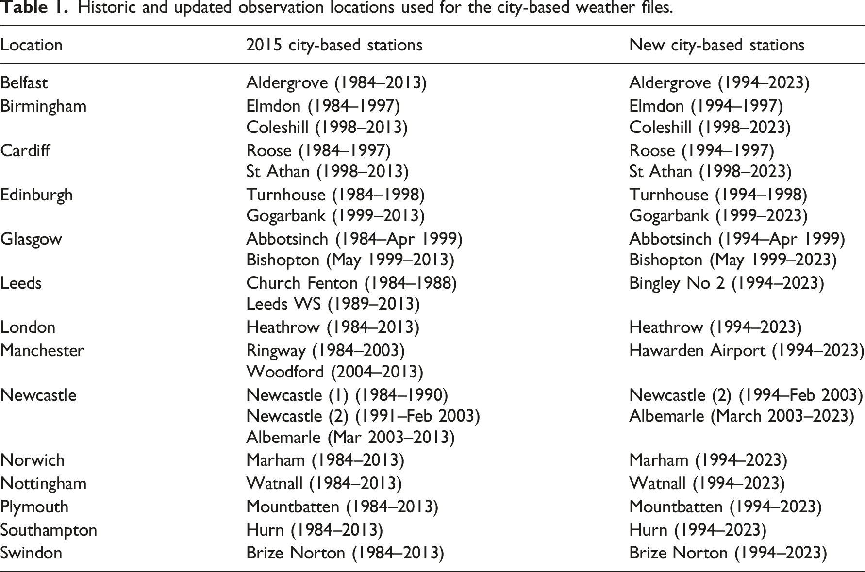
The base observation period is used to determine the months for the TRYs and the baseline observations for determining the DSYs. In the case of the DSYs, further years from the historic observations will also be used to increase the number of extreme events available. In each case this amounts to using all previous years (back to 1961) if available of the first named station. For example, in Belfast this would mean taking all observations from 1961 to 2023 for Aldergrove and for Birmingham this would mean all observations from 1961 to 1997 for Elmdon along with those from Coleshill from 1998 to 2023. In the case of London, TM49 established DSYs from rural and urban DSYs using the same years as determined from the Heathrow location. 29 TM49 used Gatwick for the rural DSYs and London Weather Station for the urban DSYs. In this case Heathrow was defined as a peri-urban site. In the update, rural DSY locations are taken from Gatwick for selected years before 1999 and Charlwood for years after. Urban DSYs come from London Weather Centre for years before 2011 and from Kew Gardens after. The peri-urban DSYs remain from Heathrow. The previous and updated locations used for baseline weather data and for determining Test Reference Years and the statistics for Probabilistic Design Summer Year are outlined in Table 1.
TRYs should consist of weather patterns which are representative of the long-term trend as observed at a particular location. Typically, Finkelstein-Schaefer (FS) statistics are used to select the appropriate months. 8 The FS statistic takes the sum of the absolute difference between an individual month’s (e.g., January) daily cumulative distribution function against the cumulative distribution using all previous months (e.g., against all previous January’s) for a given weather variable. The month with the smallest FS statistic is then taken as the month with the closest distribution to the long-term climate. This process is then followed for each month with the selected months then combined into a single TRY. The difference between various average weather files used around the world is the weather variables used to determine the average weather and depends on what is considered most important to determine building performance.
Here TRYs are created following the ISO method. 30 This method was used previously and has been described in depth elsewhere. 17 The ISO method uses dry-bulb temperature, relative humidity and solar radiation with an equal weighting to determine the 3 months with the lowest ranking (lowest weighted sum of the FS statistics). The FS statistic for wind speed is then calculated to determine the representative month. Similar to the previous update, due to the lack of directly observed solar radiation, cloud cover is used as a proxy for solar radiation in the selection of the most representative months.
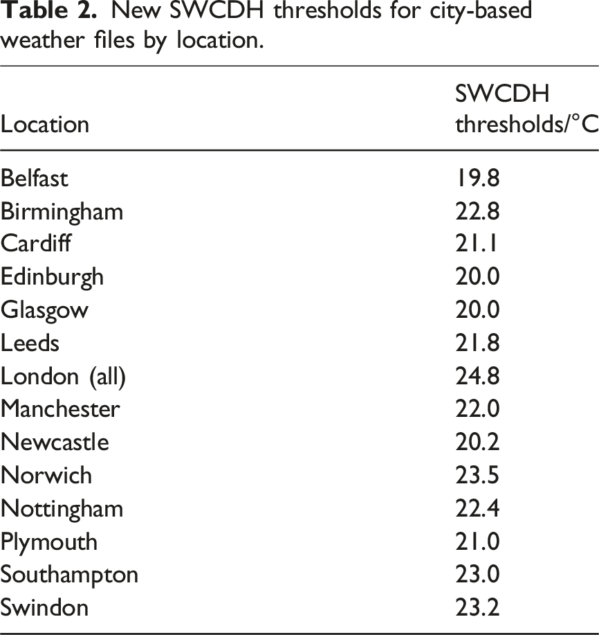
The previous method for creating DSYs involves determining extreme events, modelling these via extreme value theory to determine return period then selecting years at appropriate return periods. 31 In this work a similar approach will be used but to simplify the selection, only a single metric will be used – the Static Weighted Cooling Degree hours.
New SWCDH thresholds for city-based weather files by location.
The generation of climate zones follows the method of Xie et al where a more comprehensive description can be found. 24 A two-tiered ensemble clustering method was used to create granular climate zones in the UK, using the regional climate projections with 12 km resolution from UKCP18. The first tier identifies primary spatial climate patterns in the UK and a second-tier further segments microclimate from each primary climate zone.
A dataset of 12 model projections spanning a 100-year period (1981–2080) under the RCP8.5 emission scenario from regional projections served as the raw input for the analysis. In the first tier, 41 features were extracted from each model projection, comprising 39 climatic variables and two geographical location variables, and were used as input for the ensemble clustering model. 24 This model employed 12 base K-means models, where each projection in the dataset was assigned to a single K-means model using the bagging method. This process generated 12 variants of climate zoning results, which were then consolidated into primary climate zones through an agglomerative clustering process.
In this first step, by including geographical proximity in the clustering process, the method balances the trade-off between climate similarity and spatial continuity, resulting in compact and practical zone delineations. In total 14 climate zones were created preserving the broad spatial climate patterns experienced across the UK such as the colder north, warmer south; wetter west, and drier east, while improving local relevance.
In the second tier each climate zone was then examined in detail to identify localized microclimates. A similar clustering methodology was applied with a focus on temperature-related variables due to their significance in building performance assessments and their relevance to microclimate phenomena such as the urban heat island intensity. Specifically, three temperature variables—maximum temperature, mean temperature, and minimum temperature—were utilised for clustering.
These variables were used to further segment the microclimates within each primary climate zone. The outcome from this clustering process identified 14 climate zones which are then further segmented into 28 zones. This second clustering stage successfully captures key microclimatic areas—such as the urban heat island of London and mountainous regions—which are often overlooked in standard weather file classifications. These granular distinctions provide a more accurate reflection of local climate conditions critical for building energy modelling and a basis for further development.
However, note, the only consideration of the urban heat island intensity in the classification system is only that which is contained within the signature of the 12 km data. In many cases, urban areas would only consist of one or two grid squares at this resolution and are more anomalous than reflecting a wider climatic region within the main climate zone.
The next step is the identification of weather stations which are representative of the zone. Although the weather within the identified zones is already considered as somewhat similar by virtue of the clustering algorithm used there will be variation across the zone. A single grid cell which shows the highest similarity to the overall condition of the zone is identified to create weather files. Wasserstein distance of the climate variables between a single cell and the collection of all cells within the climate zone is employed as the selection criteria. As such, weather files created based on the selected grid cell can represent the climate condition of the whole zone.
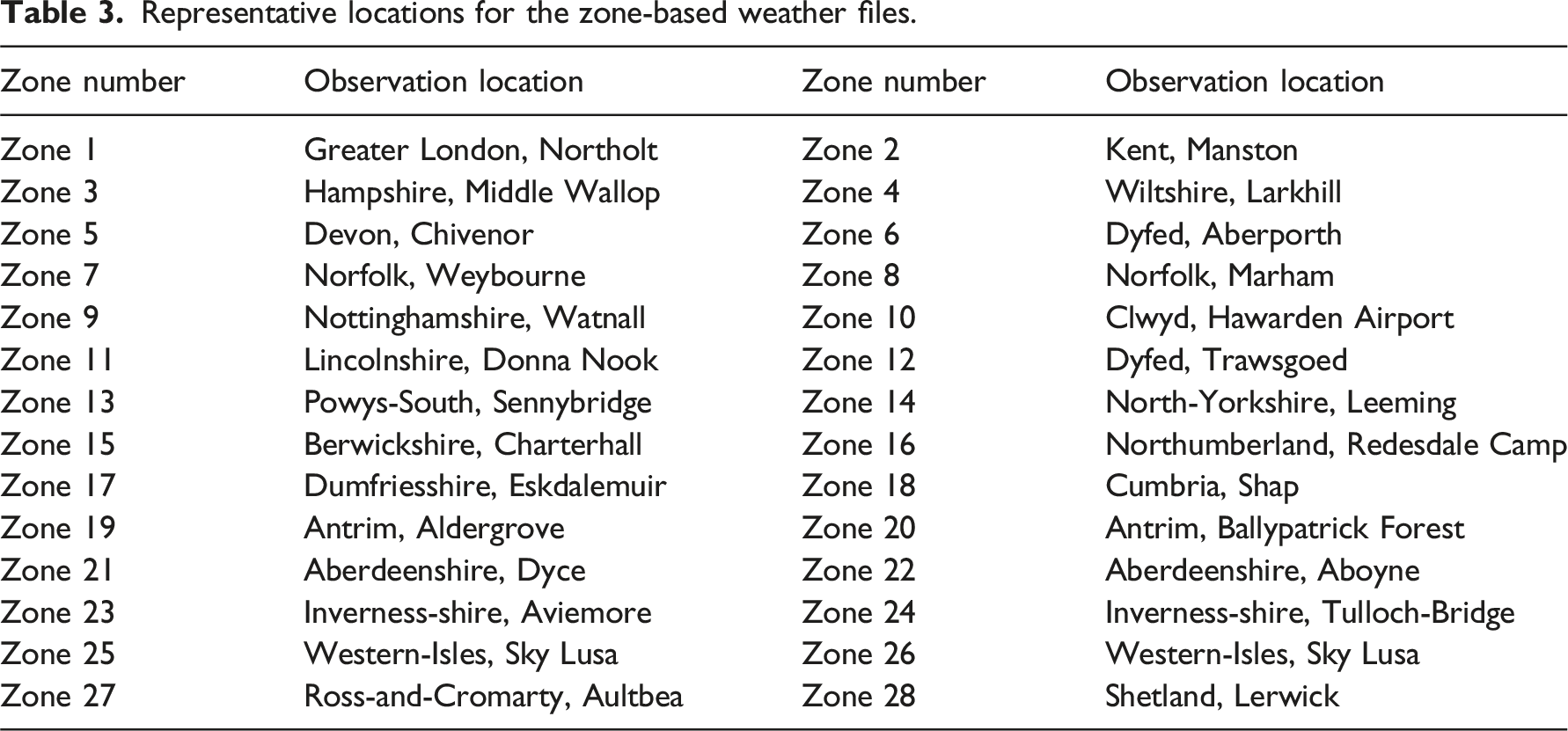
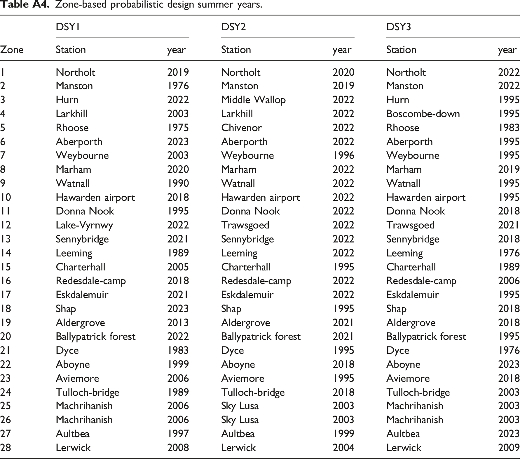
When comparing this identified grid cell with observations, ideally, a single location exists which is coherent with the identified cell. However, due to limitations in the availability of observational data, the nearest weather stations with sufficient data are used as proxies for the identified representative locations. Observation files are then generated based on these stations. Here, the representative location will be selected as the weather station with at least 20 years of suitable data for generating the base statistics which is nearest to the selected representative location (Table 3). In most cases, the selected files have the full 30 years’ worth of data from the period 1994–2023. In the case of zone 12 for example, an equivalent of 26.5 years is available but with various summer months temperature data missing, only 17 complete summers could be used to determine the baseline statistics for the DSYs.
In the case of zone 26, Inverness-shire, Aonach-Mor, would be chosen as the representative location. However, far too little observation data is available, and with no other viable weather stations within the relatively small climate zone, Sky Lusa has been used for both zone 25 and zone 26. Zone 26 was separated from zone 25 in the second tier of clustering so is somewhat representative of this zone too.
Figure 1 illustrates the climate zones (a) and the locations of the approximate regions for the city-based files (b) based on the distance away from the location. The zone-based files are fully defined with zone 1 starting around Greater London and then zone numbers generally increase going from east to west, then moving north. Hence zone 5 and 6 covers Cornwall and parts of Wales and zone 7 centres around Norfolk. Local variations are captured such as urban areas around Bristol and greater London, as well as national parks such as Dartmoor and Exmoor in the southwest, to Bannau Brycheiniog in Wales as well as the highland areas in Scotland. The largest distinction can be observed in Scotland where 12 zones are used compared to two cities. Note, to enable the city zones to be easily observed on the scale used, Greater London is assumed to use the urban London DSYs (London Weather Centre), with a surrounding ring used for the suburban file (Heathrow), with the rest of the area using the rural London file (Gatwick). Zone-based and city-based weather files and their expected usage areas. Representative locations for the zone-based weather files.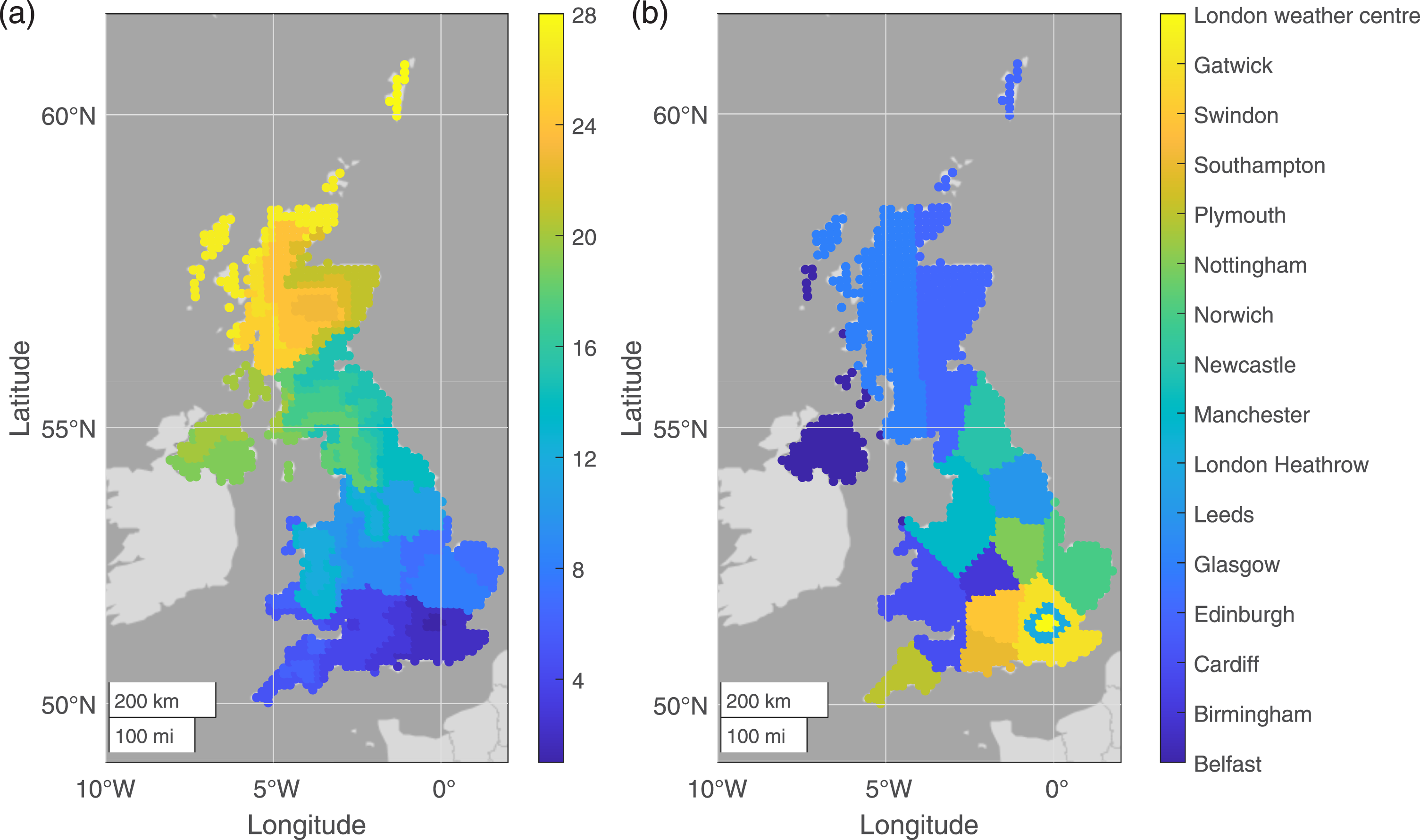
The weather files will be compared in terms of the climate expected at each location across the UK. Here we will assume that a designer would choose the closest city-based weather file to their location as often better information is not available. The climate zones have clear boundaries telling the user which file they should use. For most figures the difference between the city-based and zone-based files will be the focus. In most cases we will not adjust the weather files for altitude since the main application will be compliance modelling and therefore the results will reflect the differences between the selected files as presented. This is because this is how we expect designers to use the files in practice. For example, the National Calculation Methodology makes no reference to the need to adjust the weather file given the location but simply to select the most appropriate file. 33 In addition, standard software such would use elevation to estimate solar gains and atmospheric pressure, but not to adjust the temperature and without further automation no other adjustment would be made in practice.
The purpose of TRY files is to estimate the annual energy consumption of a building. In the UK this would be heating energy so annual heating degree days to a base of 15.5°C will be used. Part of the motivation of climate zoning is to distinguish the impacts of altitude as a result of geographical features, as evidenced by the segmented region of Exmoor, Dartmoor, Highlands, etc. Instead of correcting temperature empirically, we are using a more comprehensive method to address this issue of altitude, and other factors as well, such as proximity to sea. To distinguish the difference between the zone-based files and city files and the impact of altitude we will also calculate the heat degree days with a base of 15.5°C with all files adjusted to sea level.
On the contrary, DSYs are used to inform overheating risks and thermal discomfort during warm events. To compare the files, the annual cooling degree days with a base temperature of 15.5°C will be used. The ability of a building to remain cool during warm weather will depend on its ability to pass the likes of part O of the building regulations.14–16 Simply, we will consider the percentage of hours where the external air temperature is above the comfort temperature for category I occupants. This means that all temperatures greater than 2.5°C above the comfort temperature will be counted. This considers the acceptable range of 2°C and the effect of rounding the difference as suggested by TM52. 34
The purpose of these files will primarily be for building performance analysis so as an example we will also compare the different files from simulating a single building using EnergyPlus. The building has been used as part of a previous study and for further details readers are advised to look at Xie et al. 35 In summary the building is a two-bedroom flat with a lounge area with a total footprint of 94 m2 and a glazed area of 30.24 m2. Both the ceiling and floors are internal surfaces while the walls and windows have U-values of 0.254 W/m2/K and 1.058 W/m2/K respectively. Overall, the building is designed to be compliant with Part L of the building regulations in London. For the TRYs the average energy use through heating requirements will be output. In this set up all internal gains such as equipment, lighting, etc is removed and the energy reported will be that to keep bedrooms at 18°C and the living area at 21°C following the UK annex to BS EN 12831:2003. 30 Again, to show the impact of the zone-based approach we will also report the heating energy with all weather files adjusted for sea level.
For the use of DSYs, the ability to pass TM59 36 are seen as crucial. Here, the percentage of occupied hours where the internal operative temperature exceeds the comfort temperature will be calculated. A failure is considered when more than 3% of the occupied hours are greater than the comfort temperature. Failure is also deemed when bedroom temperatures are too high, so we will also calculate the number of hours between 22:00 and 7:00 where bedroom temperatures are above 26°C and compare these results for the two weather file location choices. Note, that TM59 considers 33 or more hours greater than 26°C as a failure. In this set up all parameter settings following CIBSE TM59. 36 When reporting the results, we only consider the worst-case exceedance across the three zones of the two bedrooms and living area.
Results
Climatic trends and variability
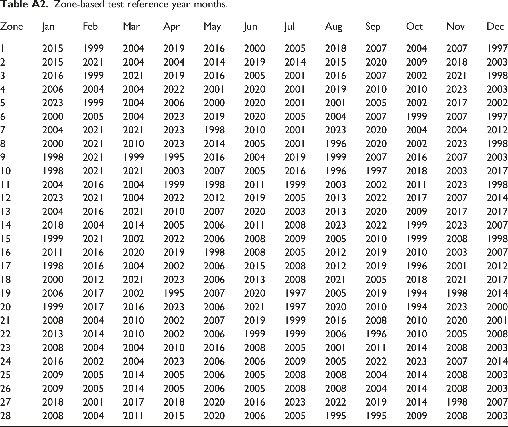
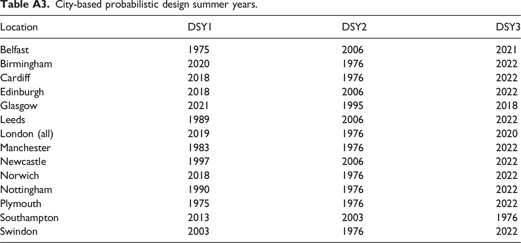
The first step of the analysis is to consider the differences in the underlying weather across all weather files. The selected weather files years for all city-based and zone-based weather files can be found in the appendix (Table A1, A2, A3 and A4). Figure 2 shows the difference between the heating degree days at the zone locations and the city-based locations with a base temperature of 15.5°C for the files as created (a) and with all files adjusted to sea level (b). A positive difference implies that the zone-based files have more heating degree days. For the files as created (Figure 2(a)) for 40% of the UK there is a difference of less than 50° days and 55% have a difference of less than 100° days. Also, for 62% of the UK the difference is very similar to the city-based degree days (within 10% of the city-based degree days). Significantly though for 17% of the UK the difference is greater than 400° days and for 5% the difference is greater than 600° days. The largest differences can be seen in some of the highland areas (around Wales, large parts of Scotland and Northern England) since these are not captured by the low resolution of the city-based files. Adjusting all files to sea level demonstrates that altitude only accounts for part of the difference and can mean anything from the zone-based files being significantly warmer to significantly cooler than the city-based equivalent. In the case of zone 24 compared to Glasgow, it reduces the difference in the HDD from +450 to −186° days implying the city location is warmer than expected given the altitude. At the other extreme comparing zone 12 to Manchester, the HDD increase from 56 to 172° days. Overall, 22% of the UK the city-based files are warmer than the zone-based files following the altitude adjustment (bigger negative difference in heating degree days) and for 78% of the UK the zone-based files would be cooler but there is no clear pattern across the UK. Looking at the HDD for the zone-based files adjusted for altitude (not shown) simply highlights the zone map as shown in Figure 1 with the highest HDD in the north and over the highlands and adjusting for altitude does not explain the difference between adjacent zones. Difference between zone-based and city-based heating degree days with a base temperature of 15.5°C for the test reference years (a) with no altitude adjustment and (b) adjusted to sea level.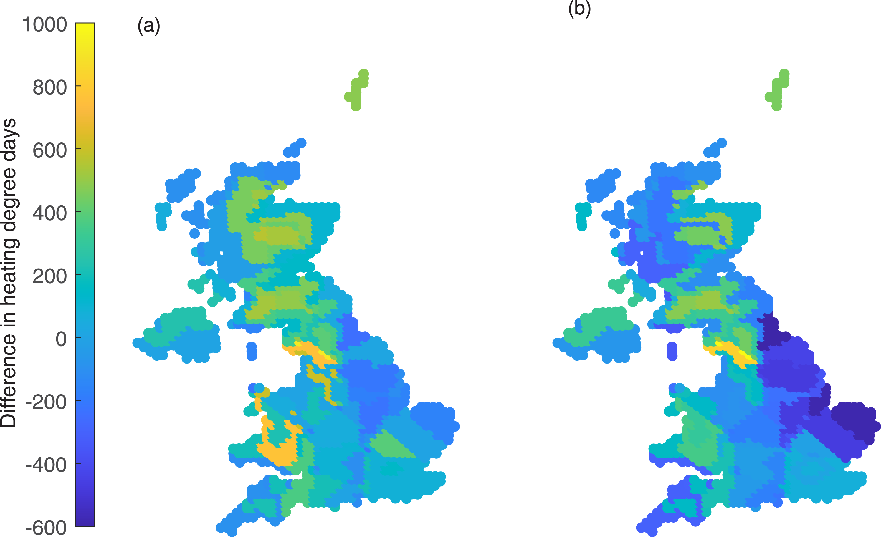
The zone-based cooling degree days with a baseline of 15.5°C can be seen in Figure 3(a)–(c) and the difference between the zone-based and city-based cooling degree days across all DSYs can be seen in Figure 3(d)–(f) for all DSYs. Again, a positive difference implies that there are more cooling degree days in the zone-based weather files than the city-based files. The highest cooling degree days can be found in the Southeast with a peak in zone 1 (Central London) for all DSYs at 383 for DSY1, 424 for DSY2 and 505 for DSY3. Generally, the cooling degree days reduces towards the West and North as well as clear reductions over moorlands and highlands. Looking at the differences between the zone-based and city-based files there is no clear pattern to which zone-based locations lead to higher cooling degree days. Overall, for 30% of the UK there is a difference of 25° days or less for all DSYS. This increases to 53%, 44% and 53% of the UK for DSY1, DSY2 and DSY3 respectively for 50°h or less. In all cases zone 1 and zone 2 are cooler than the Heathrow DSYs for all DSYs. Zone 1 is similar London Weather Centre but slightly cooler for DSYs 1 and 2 while slightly warmer for DSY3. Zone based cooling degree days (a)–(c) and the difference between zone-based and city-based cooling degree days (d)–(f) at a base temperature of 15.5°C for DSY1 (a) and (b) DSY2 (b) and (e) and DSY3 (c) and (f).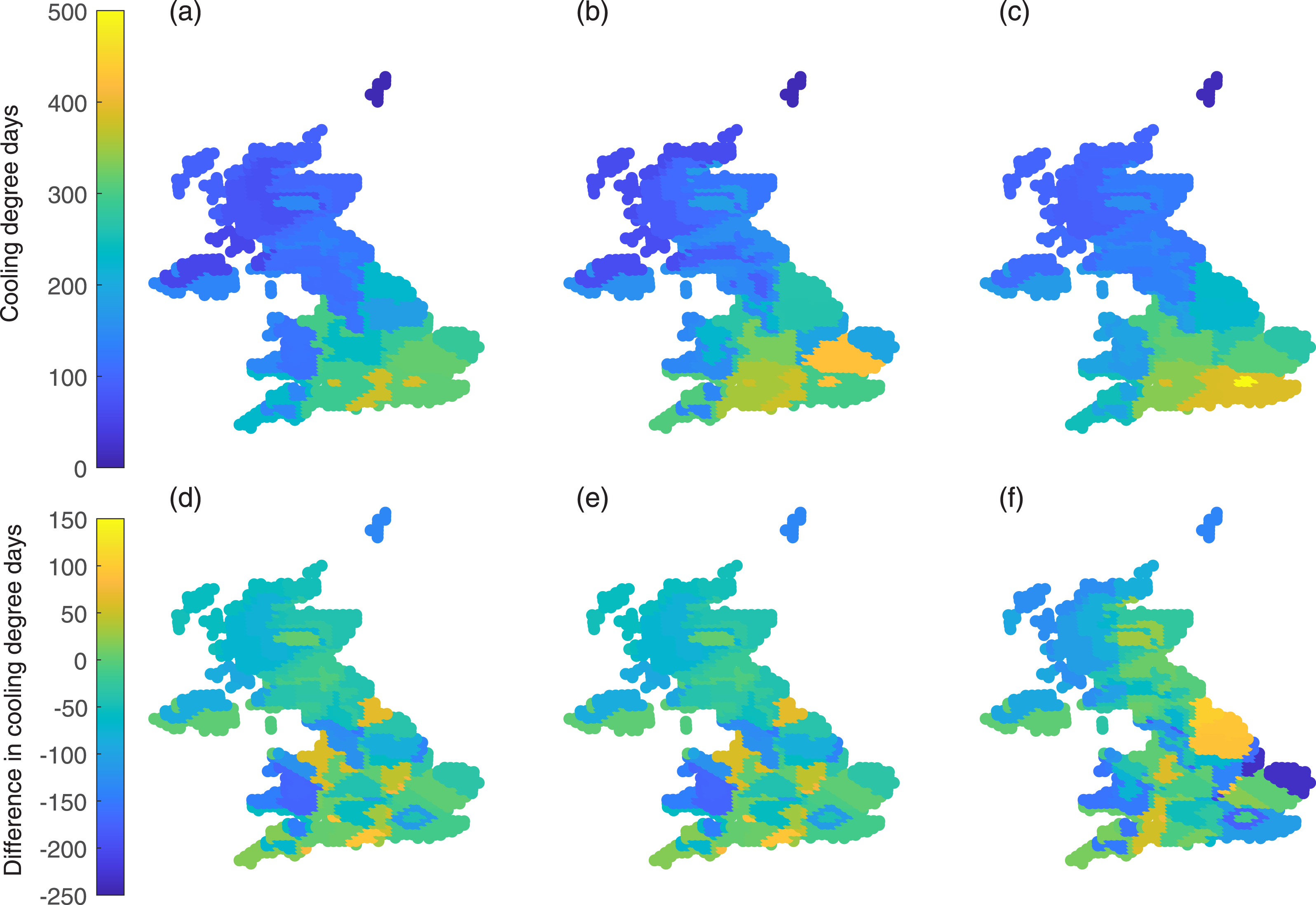
Figure 4 shows the number of hours where the external temperature exceeds the comfort temperature. For DSY1 the highest exceedance hours is 76 h (Heathrow) for the City-based files compared to 67 h (zone 1) for Zone-based files. The exceedance hours then decreases further away from the South and East. For DSY2 a similar pattern is evident with slightly more exceedance hours at all locations. The highest exceedance is 106 h for Heathrow compared to 100 h for zone 1. For the city-based files for DSY3 there is more hours of exceedance in the Southeast with a peak of 132 h for Heathrow but very few north of Manchester and Newcastle. The peak for the zone-based files and DSY3 is 106 h for zone 1. Number of hours where the external air temperature exceeds the comfort temperature for DSY1 (a) and (d), DSY2 (b) and (e) and DSY3 (c) and (f) for the zone based (a), (b) and (c) and city-based files (d), (e), (f).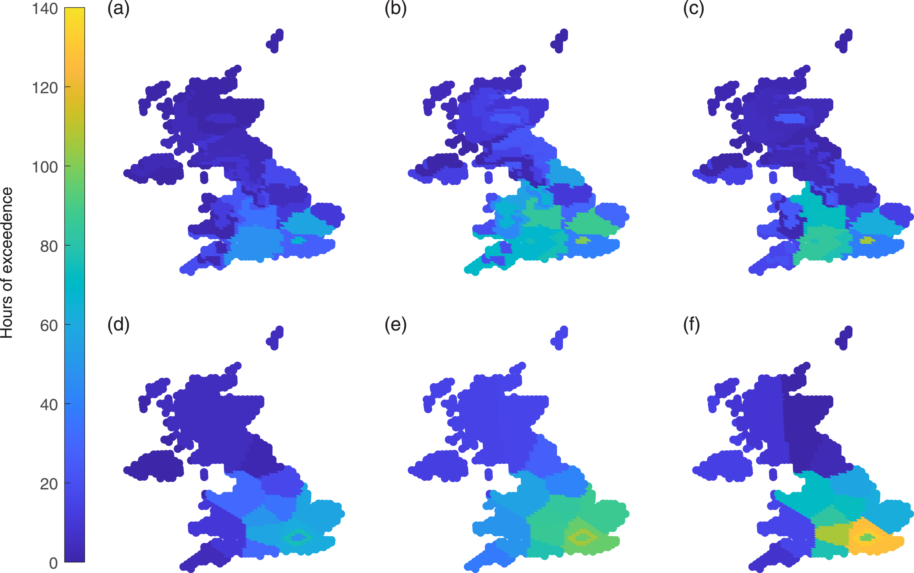
These initial results are based on the external yearly temperature distribution and do not consider the cumulative effect of warm or cool temperatures with solar radiation. While they are informative of the external climate, the impacts on building simulation are needed to complete the analysis. The simulated annual estimated heating energy using the zone-based TRYs can be seen in Figure 5(a) and the percentage difference between the zone-based and city-based files can be seen in Figure 5(b) with no altitude adjustment. Similar is seen in Figure 5(c) and (d) where the files have been scaled to sea level. For the files as created the lowest heating energy demand is 1.5 MWh for zone 5 in the Southwest and much of the South has a demand below 1.8 MWh. The heating energy then increases further north as well as over moorland and upland areas with the highest in the Shetland Islands at 3 MWh. Comparing the heating energy demand with the city-based files shows that 60% of the total area has a difference greater than 10% while 19% of the total area has a difference greater than 20%. The largest differences can be found around Dartmoor, Shetland, and the Lake District and as high as 60%. Comparing Figure 5(a) and (c) shows that adjusting the files to sea level has reduced some of the differences between some zones. The average difference in heating energy between the adjacent zones (i.e., comparing 1 and 2, 3 and 4 etc) reduces from 220 kWh to 190 kWh after adjusting for altitude. Also, the nature of the differences has no clear pattern in the changes in heating energy. Comparing 5(b) and 5(d) shows although some of the percentage differences are reduced, the differences between the city-based and zone-based files are equally not fully explained by the altitude of the zone locations. Simulated heating energy use for the zone-based TRY files (a) and (c) and the absolute percentage difference of simulated heating energy use between the city-based and zone-based TRY files (b) and (d). For (a) and (b) there is no altitude adjustment and for (c) and (d) the files are adjusted to sea level.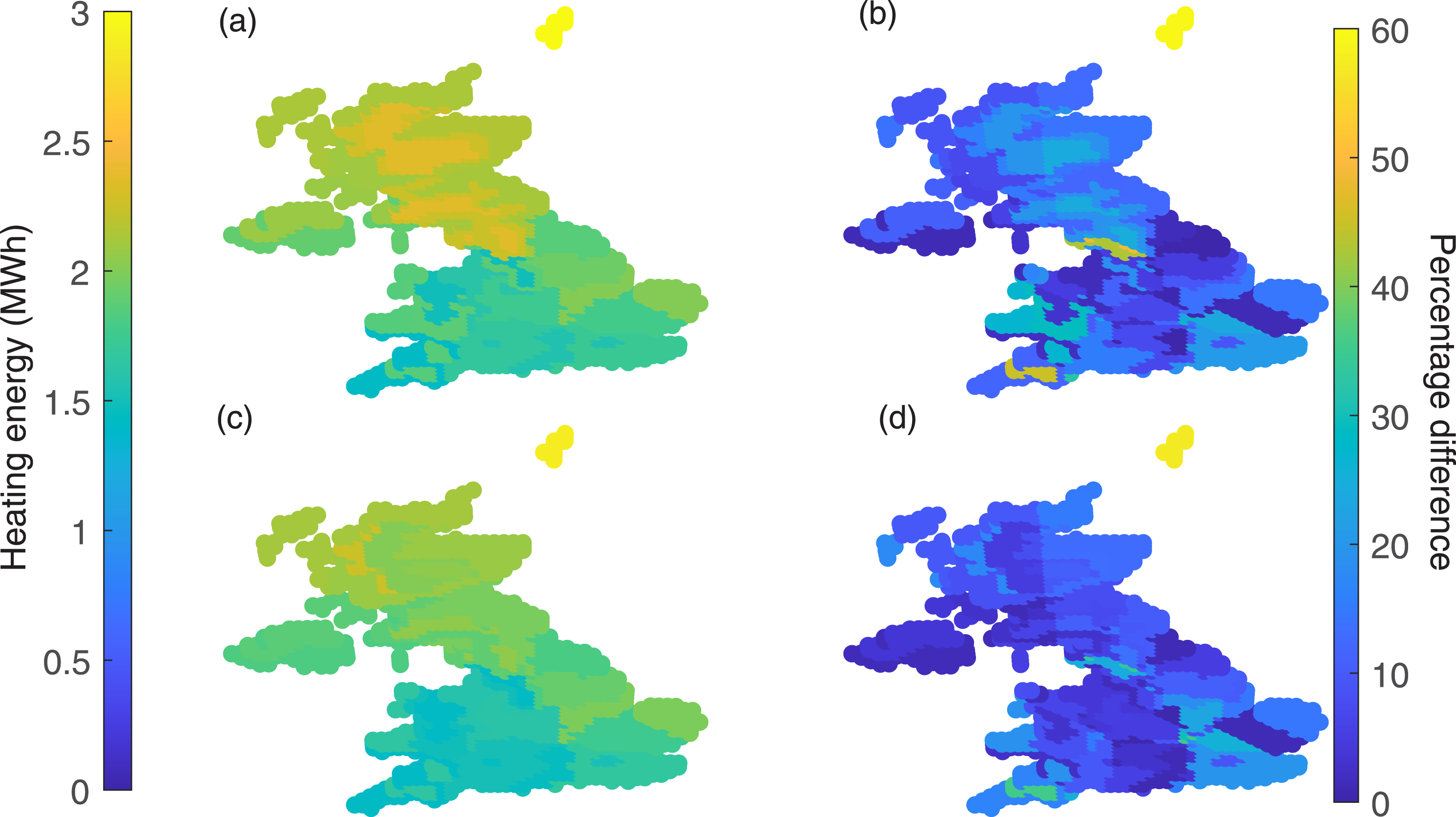
The results of the simulated percentage of occupied hours where the operative temperature exceeds the comfort criteria can be seen in Figure 6 for all DSYs and both the city-based and zone-based files. Only the room with the highest exceedance is displayed for each location. For DSY1 for both sets of weather files (Figure 6(a) and (d)) there are no locations where the exceedance is greater than 3% with a peak of 2.43% for Heathrow and 2.32% for Zone 1. For the zone-based files, 70% of the total area has less than 0.5% of occupied hours which decreases to 60% for the city-based files. For DSY2 and the city-based files (Figure 6(e)), the largest exceedance can be found around Southampton at 4% of occupied hours while both Heathrow and the London Weather Centre equally exceed 3% with 3.4% and 3.1% respectively. For the zone-based files (Figure 6(b)), all zones have an exceedance below 3% with the peak of 2.74% for zone 8 around Norfolk. For DSY3 the highest exceedance is for Heathrow at 5% (Figure 6(f)) but all London based files exceed 3% and all other locations have an exceedance below 3%. For the zone-based files (Figure 6(c)), only zone 1 exceeds 3% (3.8%). Here though, zone 23 (Aviemore) shows a much higher exceedance then the surrounding area (Cairngorms and Highlands of Scotland) at 1.25% and compared to Edinburgh (0%) or Glasgow (0.15%). Percentage of occupied hours where the operative temperature exceeds the comfort criteria for DSY1 (a) and (d), DSY2 (b) and (e) and DSY3 (c) and (f) for the zone based (a), (b) and (c) and city-based files (d), (e), (f).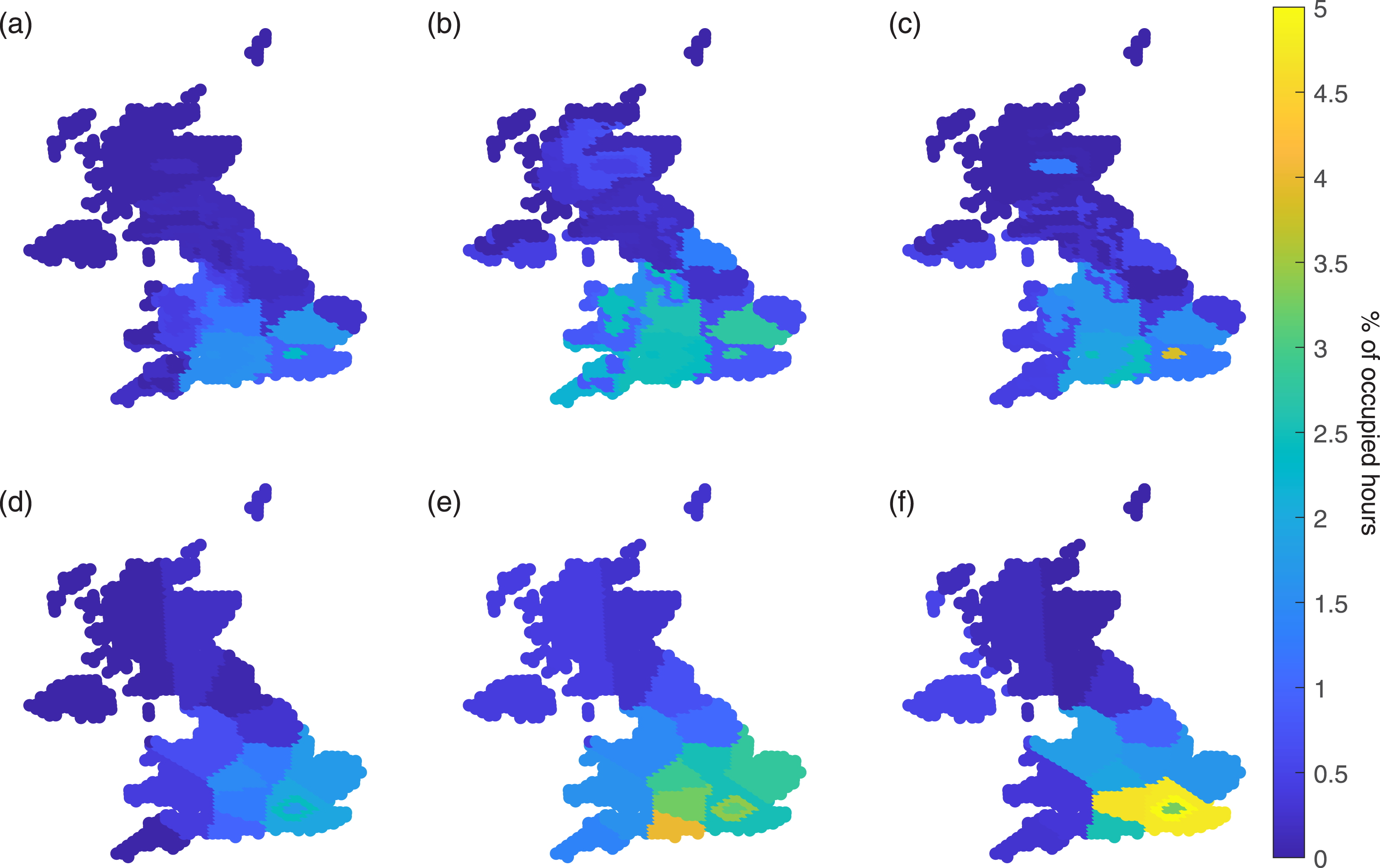
Finally, the impact on Bedroom temperatures and the hours where the bedroom is hotter than 26°C can be seen in Figure 7 for the zone based (Figure 7(a)–(c)) and the city-based (Figure 7(d)–(f)) files. For DSY1 and DSY2, for both the city-based and Zone-based files (Figure 7(a), (b), (d) and (e)) there are no locations where the bedroom fails the overheating criterion. For DSY3 both Heathrow and London Weather Centre files (Figure 7(f)) fail the criteria with 49 h greater than 26°C. The peak for the zone-based files is 14 h for zone 1 (Figure 7(c)). Overall, Figures 6 and 7 suggest that the result of London weather stations not being representative of the wider area would clearly make it harder for building designers to pass overheating assessments if the city-based files were used. Number of night-time hours where internal temperature >26°C for DSY1 (a) and (d), DSY2 (b) and (e) and DSY3 (c) and (f) for the zone based (a), (b) and (c) and city-based files (d), (e), (f).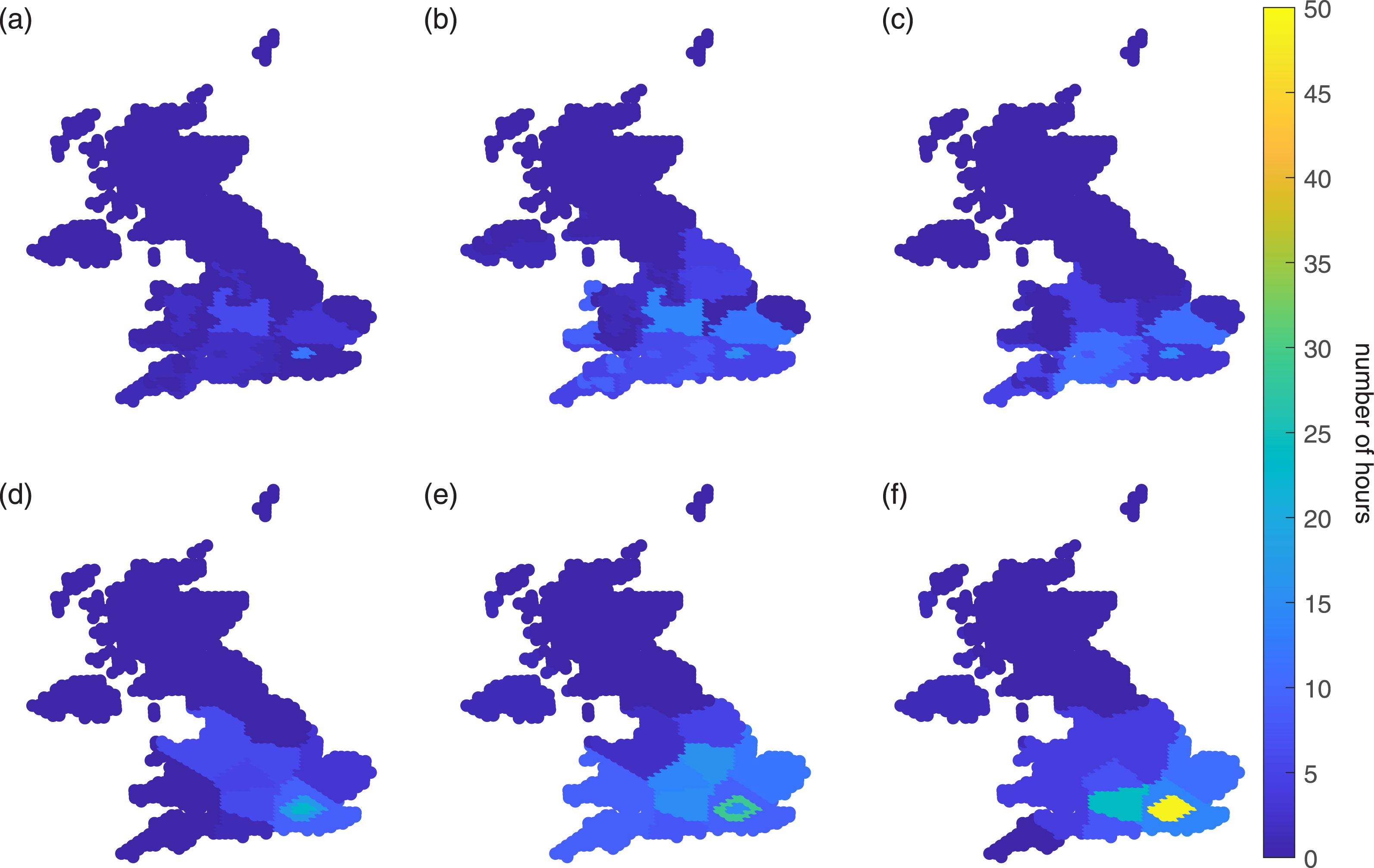
Discussion and conclusion
The analysis highlights significant differences between the city-based and zone-based files with implications for building design in terms of both heating and thermal comfort.
In terms of heating degree days, much of the differences are minimal (less than 10% difference) but in general the zone-based weather files record higher heating degree days than city-based files, particularly in highland areas such as Wales, Scotland, and Northern England, where the city-based files lack resolution and extreme variations exceeding 400° days are observed. This suggests that the city-based weather files are not representative of the wider areas that they may be used for particularly for rural locations. The differences between zones and between the city and zone-based files cannot be explained by the altitude of the files. Adjusting the files to normalise all to sea level showed that correcting the temperature empirically was not a suitable replacement for appropriate consideration of the zones as more factors such as proximity to the sea also had an influence on the zone selection.
The general pattern of the cooling degree days is as expected with a peak in the cooling degree days in central London which then decreases towards the west and north. There are some anomalies such as the cooling degree days being higher for zone 3 (378) than zone 2 (313) for DSY1. This is due to the complexity of selecting years from the different zones and then comparing adjacent zones. For example, 1976 is selected as DSY1 for zone 2 and 2022 is selected for zone 3. These results prove that the spatial pattern of the UK climate is complicated, and the current city-based files are unable to capture such diverse patterns. Within the area of Scotland alone, 12 different climate zones are involved, but the city-based weather files are only provided for two locations, i.e., Edinburgh and Glasgow. Increasing the number of sites for the city-based files would be an improvement but there would still need to be better guidance of which file to use where and the closest to the site location would not be sufficient.
The results from differences between the zone-based and city-based cooling degree days are less pronounced than for the heating degree days but this is due to the UK’s building energy demand being dominated by heating and the differences between the two files having no consistent pattern. However, the highlands and moorlands generally have fewer cooling degree days than the surrounding areas; features which again show the city-based files are not representative of the surrounding areas. Of further significance here though is the use of urban, sub-urban and rural DSYs for the London area. Heathrow is significantly warmer than any other file and is highlighted by the ring around central London. It is questionable how representative Heathrow is for any other London location and therefore its appropriateness. Here the approach of selecting a zone-based file is not to choose the hottest or coolest location but the one which is more representative of the whole zone. The point of these files is to indicate risks of overheating and to benchmark performance not to precisely predict the hours of overheating where an actual weather year derived from the climate outside the building (or nearest station) for a particular period would be more appropriate.
The thermal comfort analysis for the outside temperatures reveals notable geographic trends for both the zone-based and city-based files. In each case the highest exceedance is found in London and the exceedance reduces towards the north and west. The zone-based files again show the advantages of the higher resolution by having a reduced exceedance over the highlands and moorlands. In terms of overheating and passing TM59, the weather data indicates that if the internal temperature of the building matches the external temperature for all locations, then it would be possible to pass the overheating criteria at all locations and all weather files regardless of whether the city-based or zone-based files are used.
Extending the thermal comfort analysis to within the example building model, simulations showed that it is possible to pass TM59’s criteria for hours exceeding the comfort temperature for DSY1 for all locations and all DSY2 locations for the zone-based files. The largest exceedances are found in the Southeast with limited thermal discomfort across the rest of the country as might be expected in the UK. Similar results are found for bedroom temperatures where all zone-based files would pass the TM59 criteria and the only failure for the city-based files is for the Urban and Sub-urban files. The simulations in this example show that the amount of thermal discomfort is low but follows an expected trend – there is more thermal discomfort in the south and east and less in the north and to the west.
There is no known justification for the historically selected weather stations in the UK or then how they should be used. 8 Most have long term weather data, but this is not consistent across all locations 17 and further closures of weather stations complicate the selection of appropriate sites as found within this work, but it remains unclear how representative locations are for a specific location. Because the zone-based files have specific boundaries a clear differentiation is seen between lowland and highland regions in all results. For example, the moorlands have lower exceedance than surrounding areas reflecting the cooler climates. Similar is found in terms of estimating heating energy where larger demands are estimated in the north and highlands which has clear advantages over the city-based files where it is less certain which files should be used for which region. Here the simplest interpretation has been taken whereby the nearest weather file has been selected. This in principle follows the National Calculation Methodology modelling guide which advises the selection of the weather file corresponding to the location closest to the building site. In cases where a microclimate is present, one of the other available weather files may be used if deemed more appropriate but justification is required. 33 While the guidance emphasizes the importance of using a weather file that accurately represents the local climate, it does not provide specific instructions on how to determine the most representative file. A bigger issue arises for more remote locations where there may not be a more appropriate file. The use of climate zones removes any potential ambiguity that the use of the city-based files encounters. An approach may be to adjust the files for altitude to make the city-based files more representative, but it is clear from these results that adjusting for altitude alone does not account for the difference between zones.
In either case there are some distinct boundaries between different locations because the approach used does not provide spatial coherence since different years can be selected. Using zone-based files with observations does not solve this issue but the zones have already been shown to have long term weather data which are similar. 24 The use of observations is the limitation here. Some hot weather events such as those experienced in 2022 manifested as short, intense heat wave events in some locations (such as zones 3 and 4) but were experienced as long less intense events in neighbouring zones (zones 1 and 2) meaning different years are used across these boundaries.
The case study building model used in this work is designed to be approximately compliant with TM59 for a 2020s weather file in London, so the low levels of exceedance are to be expected. The purpose here is to show the differences between the two approaches for providing weather files and how appropriate they are for benchmarking performance. It is clear though that the zone based-files better reflect the UK climate and specific regions than the city-based files supporting their wider adoption for use in benchmarking building performance.
In conclusion, this work has shown that zone-based weather files can better support building performance analysis and compliance modelling than the historic city-based files. Having specific zones which represent microclimates with specific boundaries will support their wider use and remove uncertainty to which file is most representative of a given location. There are clear differences between both the zone-based and city-based files, but comparisons are complicated due to the lack of specific information surrounding which city-based file should be used for which location. It is also clear that elevation alone is not sufficient to explain the difference between climate zones supporting the use of the zone-based files to better reflect the building performance as well as suggesting that representative files are more suitable than empirical corrections.
The lack of consideration of what is representative about the city-based files is a clear. Heathrow for example, is a much warmer location than the surrounding areas, and our analysis shows that it is not representative of the wider zone. This work is not about making site specific weather files but demonstrates how to create weather files that can help support the development of building designs and enable benchmarking of building performance. For comparing actual performance with the local weather, an actual weather file would be needed.
Overall, the zone-based files are cooler than the city-based files. This is largely because more cooler climates are now included and warmer sites such as Heathrow, which are not representative of the wider area are not selected. In the example of the southeastern most area as represented by zone 2, a specific climate file has been established which is much cooler than the London based file that would have been used previously. This is likely to mean that less thermal discomfort will be experienced and thus less mitigation measures will be required to pass current building regulations, and in the case where mechanical cooling is employed it will result in smaller plant sizes being specified. Subsequently, resulting in lower embodied carbon or unnecessary mitigations measures being implemented in cooler regions. The imitations of this work surround the use of observations and the limited distribution of weather stations as well as the inherent issues with data quality, missing data etc. A new approach would be required to achieve spatially coherent weather files.
Footnotes
Acknowledgments
For the purpose of open access, the author has applied a Creative Commons Attribution (CC BY) licence to any Author Accepted Manuscript version arising from this submission.
Declaration of conflicting interests
The authors declared no potential conflicts of interest with respect to the research, authorship, and/or publication of this article.
Funding
The authors disclosed receipt of the following financial support for the research, authorship, and/or publication of this article: This work is funded by the Innovate UK through the Knowledge Transfer Partnerships (KTPs) programme, grant no. 12939.
Appendix
City-based test reference year months. Zone-based test reference year months. City-based probabilistic design summer years. Zone-based probabilistic design summer years.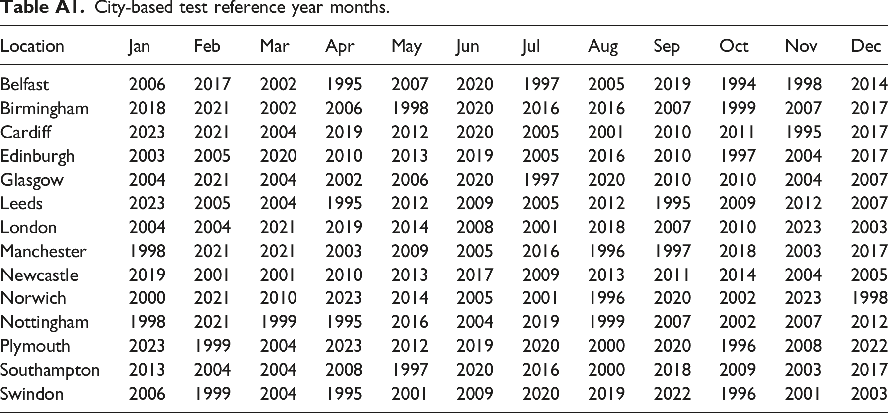
Location
Jan
Feb
Mar
Apr
May
Jun
Jul
Aug
Sep
Oct
Nov
Dec
Belfast
2006
2017
2002
1995
2007
2020
1997
2005
2019
1994
1998
2014
Birmingham
2018
2021
2002
2006
1998
2020
2016
2016
2007
1999
2007
2017
Cardiff
2023
2021
2004
2019
2012
2020
2005
2001
2010
2011
1995
2017
Edinburgh
2003
2005
2020
2010
2013
2019
2005
2016
2010
1997
2004
2017
Glasgow
2004
2021
2004
2002
2006
2020
1997
2020
2010
2010
2004
2007
Leeds
2023
2005
2004
1995
2012
2009
2005
2012
1995
2009
2012
2007
London
2004
2004
2021
2019
2014
2008
2001
2018
2007
2010
2023
2003
Manchester
1998
2021
2021
2003
2009
2005
2016
1996
1997
2018
2003
2017
Newcastle
2019
2001
2001
2010
2013
2017
2009
2013
2011
2014
2004
2005
Norwich
2000
2021
2010
2023
2014
2005
2001
1996
2020
2002
2023
1998
Nottingham
1998
2021
1999
1995
2016
2004
2019
1999
2007
2002
2007
2012
Plymouth
2023
1999
2004
2023
2012
2019
2020
2000
2020
1996
2008
2022
Southampton
2013
2004
2004
2008
1997
2020
2016
2000
2018
2009
2003
2017
Swindon
2006
1999
2004
1995
2001
2009
2020
2019
2022
1996
2001
2003
Zone
Jan
Feb
Mar
Apr
May
Jun
Jul
Aug
Sep
Oct
Nov
Dec
1
2015
1999
2004
2019
2016
2000
2005
2018
2007
2004
2007
1997
2
2015
2021
2004
2004
2014
2019
2014
2015
2020
2009
2018
2003
3
2016
1999
2021
2019
2016
2005
2001
2016
2007
2002
2021
1998
4
2006
2004
2004
2022
2001
2020
2001
2019
2010
2010
2023
2003
5
2023
1999
2004
2006
2000
2020
2001
2001
2005
2002
2017
2002
6
2000
2005
2004
2023
2019
2020
2005
2004
2007
1999
2007
1997
7
2004
2021
2021
2023
1998
2010
2001
2023
2020
2004
2004
2012
8
2000
2021
2010
2023
2014
2005
2001
1996
2020
2002
2023
1998
9
1998
2021
1999
1995
2016
2004
2019
1999
2007
2016
2007
2003
10
1998
2021
2021
2003
2007
2005
2016
1996
1997
2018
2003
2017
11
2004
2016
2004
1999
1998
2011
1999
2003
2002
2011
2023
1998
12
2023
2021
2004
2022
2012
2019
2005
2013
2022
2017
2007
2014
13
2004
2016
2021
2010
2007
2020
2003
2013
2020
2009
2017
2017
14
2018
2004
2014
2005
2006
2011
2008
2023
2022
1999
2023
2007
15
1999
2021
2002
2022
2006
2008
2009
2005
2010
1999
2008
1998
16
2011
2016
2020
2019
1998
2008
2005
2012
2019
2010
2003
2007
17
1998
2016
2004
2002
2006
2015
2008
2012
2019
1996
2001
2012
18
2000
2012
2021
2023
2006
2013
2008
2021
2005
2018
2021
2017
19
2006
2017
2002
1995
2007
2020
1997
2005
2019
1994
1998
2014
20
1999
2017
2016
2023
2006
2021
1997
2020
2010
1994
2023
2000
21
2008
2004
2010
2002
2007
2019
1999
2016
2008
2010
2020
2001
22
2013
2014
2010
2002
2006
1999
1999
2006
1996
2010
2005
2008
23
2008
2004
2004
2010
2016
2008
2005
2001
2011
2014
2008
2003
24
2016
2002
2004
2023
2006
2006
2009
2005
2022
2023
2007
2014
25
2009
2005
2014
2005
2006
2005
2008
2008
2004
2014
2008
2003
26
2009
2005
2014
2005
2006
2005
2008
2008
2004
2014
2008
2003
27
2018
2001
2017
2018
2020
2016
2023
2022
2019
2014
1998
2007
28
2008
2004
2011
2015
2020
2006
2005
1995
1995
2009
2008
2003
Location
DSY1
DSY2
DSY3
Belfast
1975
2006
2021
Birmingham
2020
1976
2022
Cardiff
2018
1976
2022
Edinburgh
2018
2006
2022
Glasgow
2021
1995
2018
Leeds
1989
2006
2022
London (all)
2019
1976
2020
Manchester
1983
1976
2022
Newcastle
1997
2006
2022
Norwich
2018
1976
2022
Nottingham
1990
1976
2022
Plymouth
1975
1976
2022
Southampton
2013
2003
1976
Swindon
2003
1976
2022
Zone
DSY1
DSY2
DSY3
Station
year
Station
year
Station
year
1
Northolt
2019
Northolt
2020
Northolt
2022
2
Manston
1976
Manston
2019
Manston
2022
3
Hurn
2022
Middle Wallop
2022
Hurn
1995
4
Larkhill
2003
Larkhill
2022
Boscombe-down
1995
5
Rhoose
1975
Chivenor
2022
Rhoose
1983
6
Aberporth
2023
Aberporth
2022
Aberporth
1995
7
Weybourne
2003
Weybourne
1996
Weybourne
1995
8
Marham
2020
Marham
2022
Marham
2019
9
Watnall
1990
Watnall
2022
Watnall
1995
10
Hawarden airport
2018
Hawarden airport
2022
Hawarden airport
1995
11
Donna Nook
1995
Donna Nook
2022
Donna Nook
2018
12
Lake-Vyrnwy
2022
Trawsgoed
2022
Trawsgoed
2021
13
Sennybridge
2021
Sennybridge
2022
Sennybridge
2018
14
Leeming
1989
Leeming
2022
Leeming
1976
15
Charterhall
2005
Charterhall
1995
Charterhall
1989
16
Redesdale-camp
2018
Redesdale-camp
2022
Redesdale-camp
2006
17
Eskdalemuir
2021
Eskdalemuir
2022
Eskdalemuir
1995
18
Shap
2023
Shap
1995
Shap
2018
19
Aldergrove
2013
Aldergrove
2021
Aldergrove
2018
20
Ballypatrick forest
2022
Ballypatrick forest
2021
Ballypatrick forest
1995
21
Dyce
1983
Dyce
1995
Dyce
1976
22
Aboyne
1999
Aboyne
2018
Aboyne
2023
23
Aviemore
2006
Aviemore
1995
Aviemore
2018
24
Tulloch-bridge
1989
Tulloch-bridge
2018
Tulloch-bridge
2003
25
Machrihanish
2006
Sky Lusa
2003
Machrihanish
2003
26
Machrihanish
2006
Sky Lusa
2003
Machrihanish
2003
27
Aultbea
1997
Aultbea
1999
Aultbea
2023
28
Lerwick
2008
Lerwick
2004
Lerwick
2009