
Abstract
Lithium-ion batteries have been widely used in electric vehicles, smart grids and many other applications as energy storage devices, for which the aging assessment is crucial to guarantee their safe and reliable operation. The battery capacity is a popular indicator for assessing the battery aging, however, its accurate estimation is challenging due to a range of time-varying situation-dependent internal and external factors. Traditional simplified models and machine learning tools are difficult to capture these characteristics. As a class of deep neural networks, the convolutional neural network (CNN) is powerful to capture hidden information from a huge amount of input data, making it an ideal tool for battery capacity estimation. This paper proposes a CNN-based battery capacity estimation method, which can accurately estimate the battery capacity using limited available measurements, without resorting to other offline information. Further, the proposed method only requires partial charging segment of voltage, current and temperature curves, making it possible to achieve fast online health monitoring. The partial charging curves have a fixed length of 225 consecutive points and a flexible starting point, thereby short-term charging data of the battery charged from any initial state-of-charge can be used to produce accurate capacity estimation. To employ CNN for capacity estimation using partial charging curves is however not trivial, this paper presents a comprehensive approach covering time series-to-image transformation, data segmentation, and CNN configuration. The CNN-based method is applied to two battery degradation datasets and achieves root mean square errors (RMSEs) of less than 0.0279 Ah (2.54%) and 0.0217 Ah (2.93% ), respectively, outperforming existing machine learning methods.
Keywords
Introduction
Due to continual falling costs, and features of high energy density, low self-discharge rate and long lifespan relative to other battery types, Lithium-ion batteries have been widely used as energy storage devices for electric vehicles (EVs), electric power grid, portable electronic devices, and many other applications (Li et al., 2019a; Zhang et al., 2016). However, undesirable side reactions and processes inside the batteries while in use will continuously degrade their performance, leading to capacity loss and increase of internal resistance (Couto et al., 2019). Therefore, battery capacity and internal resistance are two important indicators for assessing battery ageing and performance degradation known as battery state of health (SOH). For example, SOH can be defined as
Accurate capacity estimation provides insights into the SOH, thus plays a critical role in the battery management system, ensuring safe and reliable battery operation, preventing incipient failures and catastrophic hazards, and prolonging the battery service life (Liu et al., 2019b). However, the battery capacity can not be measured in real time, and a variety of estimation/prediction methods have been developed (Tang et al., 2019). These methods can generally be classified into three categories: model-based, differential analysis-based, and machine learning-based.
Model-based methods use battery electrochemical, electrical, or other empirical models to depict the battery dynamics, and estimate the battery capacity with a combination of observers or adaptive filtering algorithms (Garg et al., 2018; Ouyang et al., 2016). A comprehensive review of battery modelling methods including electrochemical models, reduced-order models, equivalent circuit models, empirical models and black-box models has been presented by Zhang et al. (2014). Liu et al. (2020a) have systematically evaluated the performance of three modelling techniques (i.e. electrochemical model, semi-empirical model and Gaussian process regression-based model) for calendar ageing prediction in terms of accuracy, generalization ability and uncertainty management. Zheng et al. (2016) propose to estimate the battery capacity by using proportional integral observers based on an accurate electrochemical model, which can capture the spatiotemporal dynamics of batteries based upon the electrochemical principles. The equivalent circuit model with online identified parameters is used by Yu et al. (2019), and based on this model, an adaptive H infinite filter is applied to estimate the battery capacity. An empirical model that can reflect the battery dynamic capacity fading is proposed to predict the capacity degradation (Xu et al., 2016). However, the accuracy of the model-based capacity estimation methods is dependent on the quality of the estimation model. Unfortunately, it is difficult to build precise battery models due to the complex electrochemical reactions inside the battery under different operation conditions. Given the sheer complexity of the ageing mechanisms, simple lumped parameter models will lead to inaccurate estimation of the battery capacity.
The differential analysis-based methods correlate the features extracted from the differentiated curves of some electrical, thermal or mechanical parameters with battery capacity fade. For example, incremental capacity (IC) analysis and differential voltage (DV) analysis have been frequently used (Xiong et al., 2018). IC is calculated by differentiating the capacity change corresponding to its terminal voltage (dQ/dV) through charging or discharging the battery under a small and constant current rate. The DV curves (dV/dQ) is defined as the inverse of IC. The voltage plateaus can be easily identified from the IC/DV curves (peaks/valleys) after the differential operation. The features extracted from the curves such as IC peak position, peak shape, corresponding peak voltage/SOC, and peak area, are analyzed to estimate the battery capacity. For example, Li et al. (2018) have extracted five different features from the IC curves, the first two are peaks and the last two are valleys, the rest is the shoulder of the IC curves. The capacity is estimated by analyzing the position, value and associated area changes of these features. As described in Weng et al. (2016), the IC peak values are tracked to estimate the capacity for single cells as well as battery packs. In Zheng et al. (2018), three corresponding SOC positions are extracted from the SOC-based IC and DV curves for battery capacity estimation. While Tang et al. (2018) use a regional voltage, which is calculated by the terminal voltage corresponding to the IC peak, for fast capacity estimation. However, the IC/DV analysis is sensitive to measurement noise and subject to operation temperature, further, it requires very low current rate, therefore their applications are severely constrained (Li et al., 2019b).
With the unprecedented progress of machine learning (ML) techniques and the documentation of a large volume of battery test data worldwide, ML techniques have shown a greater potential in benefiting the battery capacity estimation. These methods are model-free, and do not need prior knowledge on the complex working principles of the battery. Various ML techniques have been applied to estimate the battery capacity fade, such as neural networks (NNs) (Dai et al., 2018; You et al., 2016; Zhang et al., 2019), recurrent neural network (RNN) (Chaoui and Ibe-Ekeocha, 2017; Eddahech et al., 2012), support vector machine (SVM) (Liu et al., 2018), support vector regression (SVR) (Weng et al., 2013), and relevance vector machine (RVM) (Guo et al., 2019; Hu et al., 2015), just to name a few. In You et al. (2016), a NN with various optimization strategies is used for capacity estimation, by combining with the k-means clustering algorithm, achieving a RMSE of less than 2.44%. The inputs fed into this NN are the features manually extracted from the raw data. The RNN is used to predict the battery performance degradation in Eddahech et al. (2012), the mean square errors for capacity and resistance prediction are 0.462 and 0.296, respectively. In Liu et al. (2018), the nonlinear relationship between the extracted battery degradation features and battery capacity is established using the least square SVM method. The mean error for the capacity estimation is less than 5%. In Weng et al. (2013), a linear programming-based SVR is proposed to correlate the IC peaks with the faded battery capacity, the model developed using one cell data is able to estimate the capacity fade of other cells with absolute error less than 1%. In Guo et al. (2019), a RVM based on particle swarm optimization is used to predict the battery capacity by modelling the relationship between the health feature and capacity, a relative error of less than 5% and 10% is achieved for single and multiple battery experiments respectively. In Eleftheroglou et al. (2019), three ML-based methods are used for battery health prediction, and the uncertainty associated with each point prediction is quantified. Liu et al. (2020b) have proposed a hybrid method for battery capacity and remaining useful life prediction, where the long short term memory model is used to capture the long-term capacity degradation dynamics and the Gaussian process regression model is used for the uncertainty quantification caused by the capacity regeneration phenomena. Further, the convolutional neural network (CNN) is applied to estimate the battery capacity using the measured voltage, current and the calculated cumulative capacity as inputs, of which the overall RMSEs are less than 2% on the NASA dataset (Shen et al., 2019).
However, the aforementioned ML-based estimation methods require either a non-trivial health features extraction process or an extra cumulative capacity calculation process, rather than directly use the measurements (e.g. current, terminal voltage, surface temperature). In summary, the battery capacity estimation is still a challenging topic due to a range of time-varying situation-dependent internal and external factors. Traditional simplified models and ML tools are difficult to capture these characteristics. As a class of deep NNs, CNN is powerful to capture hidden information from a huge amount of input data, making it an ideal tool for battery capacity estimation. In order to make full use of the information embedded in the direct measurements, while eliminating the necessity to manually extract features as well as fully charge a battery from a pre-defined state-of-charge, this paper proposes a CNN-based battery capacity estimation method using partial charging segment with flexible starting point. The paper has the following four contributions:
Firstly, the CNN-based method will eliminate the need for priori knowledge and accurate battery physical model, making the method intelligent and adaptive for real-time capacity estimation.
Secondly, the proposed method can deal with raw signals directly, mapping the measurements such as the terminal voltage, current, and surface temperature to the battery capacity, instead of relying on the pre-extracted health features. The representative features will be automatically learnt from the raw data.
Thirdly, the paper introduces a novel data segmentation and time series-to-image transformation method which makes it feasible to use CNN for battery capacity estimation. Further, the proposed method only requires flexible partial charging segment of voltage, current and surface temperature curves, allowing fast and accurate capacity estimation, a key issue in real-time battery management.
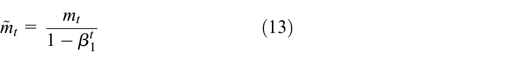
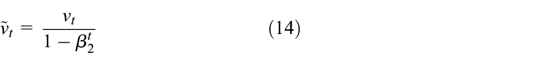
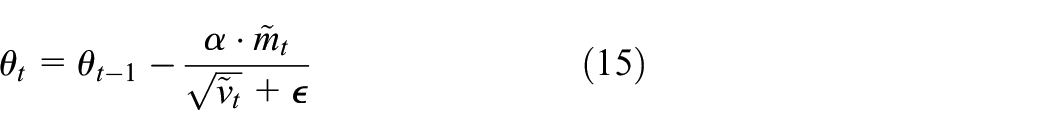
Finally, the proposed CNN-based method can self-learn its parameters and weights by using optimization algorithms like Adam. Once the parameters are properly learned offline, the model can be directly applied for fast online estimation.
The remainder of this paper is organized as follows. In Section 2, a brief introduction of the CNN is presented. Section 3 details the proposed CNN-based battery capacity estimation method, including the signal-to-image transformation method and the proposed CNN architecture. Section 4 validates the proposed method on two battery degradation data-sets and the experimental results are presented and analyzed. Finally, Section 5 concludes the paper.
CNN
Overview
The CNN is probably one of the most popular NNs in recent years. Compared with traditional deep neural networks (DNNs) with the same number of layers, the number of parameters (weights) of a CNN that are required to maintain the accuracy is significantly reduced, due to the sparse connectivity, shared weights, and pooling architectures. The sparse connectivity is achieved by making the size of filter smaller than the input, and enforcing a local connectivity pattern among neurons of adjacent layers. This architecture can reduce the overfitting risk, because the number of parameters are dramatically reduced. Shared weights refers to using the same weights for more than one activation function in a model, that is, each filter is used across the whole visual field. The architecture of shared weights has endowed the CNN with a property called equivariance, meaning that the output will change in the same way as the input changes (Liu et al., 2017). Then, the use of pooling architecture replaces the outputs of the convolutional layer with summary statistic, and this subsampling operation makes the output insensitive to small translation of the input.
CNNs are effective tools for extracting features from a high-dimensional data, and have been widely used in a range of fields, such as image processing, text classification, and speech recognition. These high-dimensional signals usually have high spatial or temporal correlations in adjacent variables, which can be effectively extracted through the convolution operations. Due to the fact that time series data is ubiquitous and is constantly generated in many engineering processes and in our daily life, there are imperative needs to develop efficient techniques to extract useful information from time series data. Considering the merits of CNNs in terms of automatic feature extraction and low overfitting risk, their applications in dealing with large amount of time series signals have also been investigated. For example, some reports have confirmed the potential of CNNs in extracting the representative features from time series data. In Yang et al. (2015), a CNN is used for solving a human activity recognition problem where the inputs of the network are multichannel time series signals collected from inertial sensors, and the outputs are related human activities. In this application, the filters in the CNN move along the temporal dimension for each sensor (each sensor corresponds to a row in the two-dimensional (2D) input). In Cui et al. (2016), a multi-scale CNN is used for time series data classification problems. The CNN architecture has multiple branches in its first layer that can extract features of different frequency and time scales. Further, CNNs have also been used for time series forecasting and estimation, and fault diagnosis.
CNN architecture
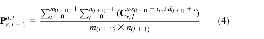
A three-layer fully connected feedforward neural network and a simple CNN are compared in Figure 1. To illustrate the differences in neuron connection between conventional neural networks and CNNs, Figure 1(b) reformulates the 2D input into a column, it is obvious that each output node in a convolutional layer is connected to a small subset of the inputs. This sparse connectivity is different from the fully connected NNs, and this sparsity is achieved by replacing the matrix multiplication in NNs with convolutions (Borovykh et al., 2017). The filter (also called weight matrix) slides over the input space and generates a set of output nodes, and each output node is calculated by convolving the input with the filter. The number of involved inputs for one output node is dependent on the filter size. All the output nodes produced by the same filter form a feature map, which is a matrix, while the number of feature maps is decided by the number of filters. In other words, all the nodes in one output feature map share the same weights. For the
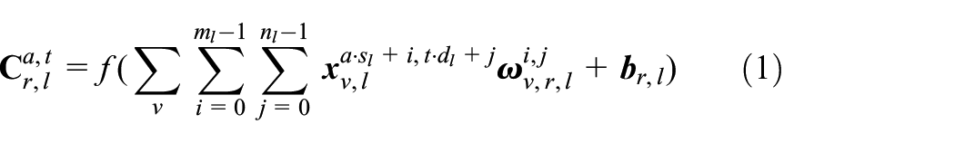
where
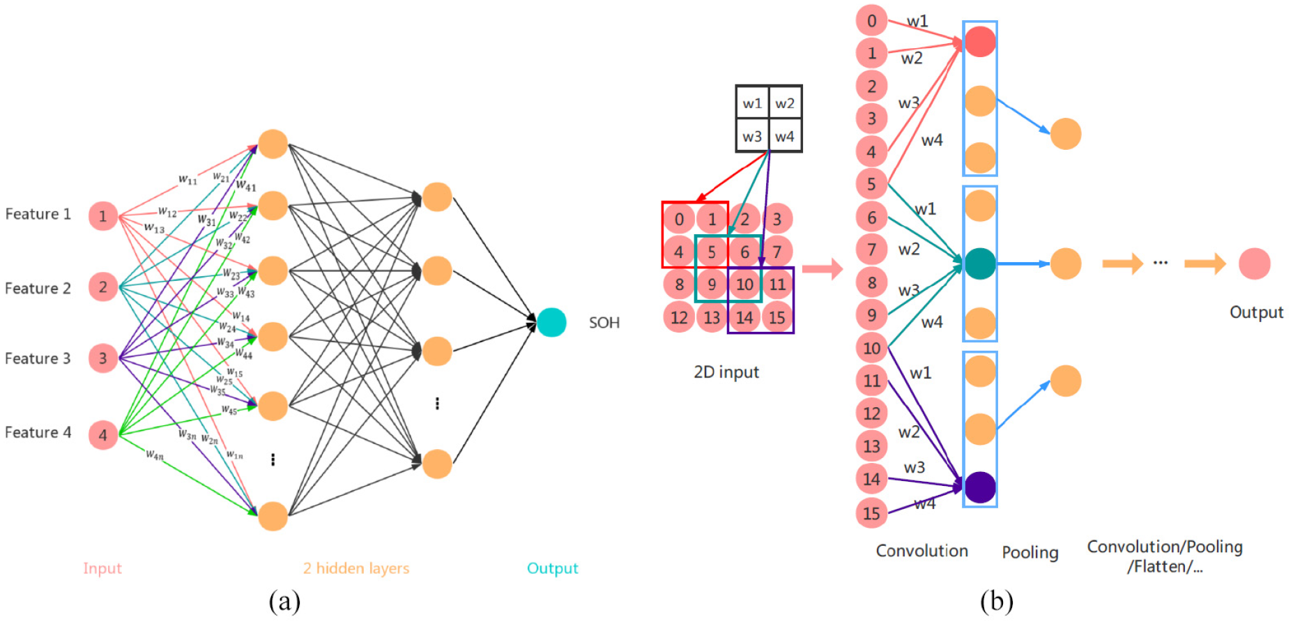
(a) A fully connected three-layer feedforward neural network. (b) A CNN, with convolutional layer as the first layer and pooling layer as the second layer. Here, the filter size is 2×2 with stride (1,1), and the pooling size is 1×3 with stride (1,1).
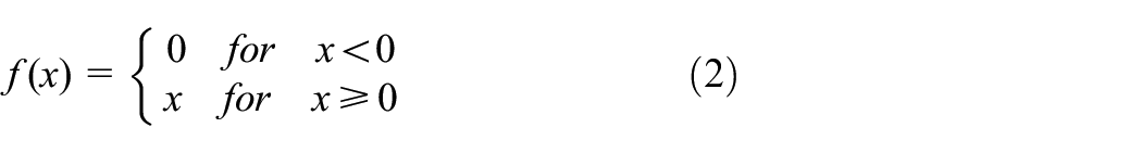
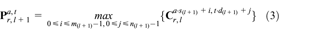
The pooling layer is a down-sampling process which reduces the size of the feature maps extracted in a convolution layer as well as the number of parameters introduced to the following layers by either max pooling strategy
or average pooling strategy
where
In the example shown in Figure1(b), only one filter is used, the filter size is
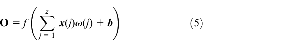
where


where
All the weights and bias are tunable parameters (


where
Methodology
In this section, the proposed CNN-based battery capacity estimation method is described in detail. First, the method to transform the measured time series signals consisting of battery current, terminal voltage and cell temperature to a 3D image representation is introduced. Then the CNN is designed based on the classical LeNet-5 configuration (LeCun et al., 1998).
Time series signal transformation
For other popular capacity estimation methods, the measurement data are not directly used for capacity estimation, and some features need to be extracted from the data first. For these methods, the estimation performance is dependent on both the number of extracted features and the way they are combined (Cai et al., 2019). However, it is not easy to effectively and efficiently extract features form the raw data. To make full use of the large volume of historic measurements, the correlations among different measured variables at different sampling periods have to be investigated. This is, however, not a trivial task to handle manually. CNNs, however, can overcome this difficulty, but to apply CNN for capacity estimation, a transformation stage is first required, which is elaborated below.
As illustrated in Figure 2, which shows one complete charging and discharging cycle,
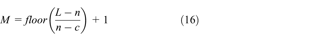
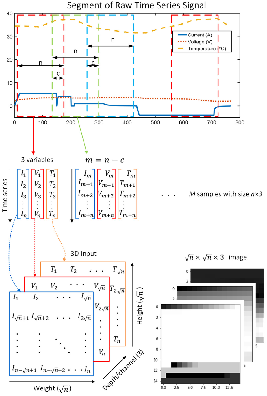
Transformation method: convert the time series measurements to 3-D images.
The function floor(.) gives the greatest integer less than or equal to the input parameter. The samples generated from the same cycle correspond to the same capacity value. Since each sample intercepted from the full charging and discharging cycle corresponds to a part of the charging/discharging process, based on the model trained with such samples, it is possible to estimate the capacity of a battery only using a part of the charging/discharging data. Besides, the part of the charging/discharging curve intercepted from the whole cycle may start at any point, meaning that the trained model can estimate the capacity of the battery charged/discharged from any unknown initial SOC.
As shown in Figure 2, these measurements have different scale, which may slow the training process and degrade the estimation accuracy. Thus, data normalization is applied to process the signals before feed them into the network. In this work, the min-max normalization strategy is adopted, which retains the original distribution of data and all transformed data fall into the range of [-1,1], reflecting both the charging and discharging phases. The normalized value
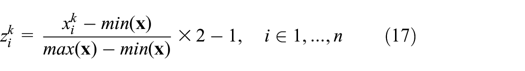
where
After the data normalization and time series to image transformation step, the final input of the CNN is illustrated in Figure 3. This data transformation method is simple to use because no predefined parameters are required, and it is an enabling block to apply the CNNs for time series signals.
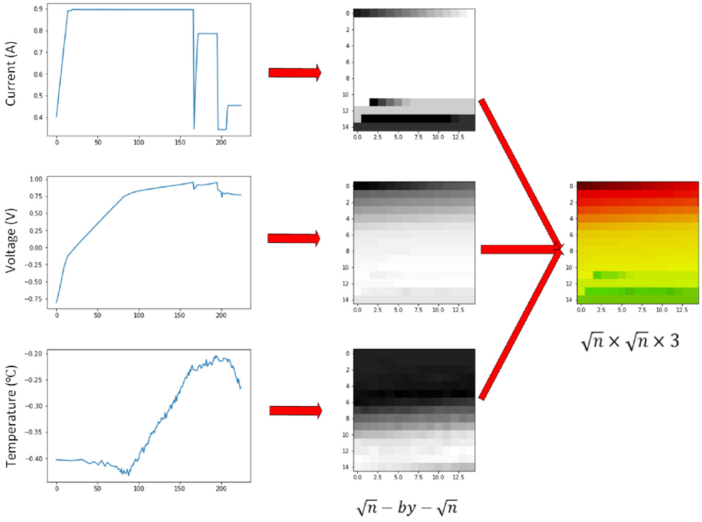
The input of the proposed CNN.
Model construction
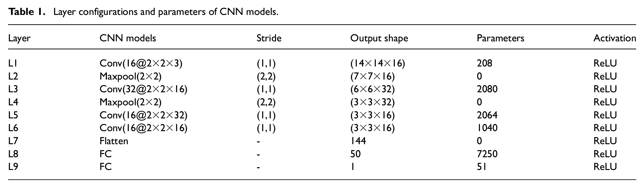
With the transformed 3D data, the CNN can then be trained to estimate the battery capacity. Considering that the size of the input sample is relatively small (
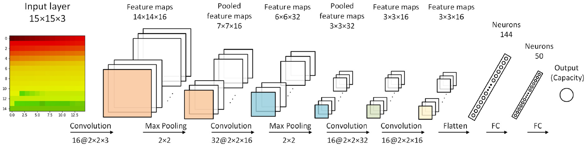
Proposed CNN architecture with
Layer configurations and parameters of CNN models.
Experiment and analysis
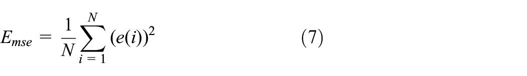
In this section, the proposed CNN-based capacity estimation method is applied to two battery experimental datasets. The first is sourced from 124 commercial lithium-ion batteries cycled to failure under fast-charging conditions (Severson et al., 2019), and the other is the Oxford Battery Degradation Dataset (Birkl, 2017). During the training process, the number of the maximum training epochs is set to 80 and the mini-batch size is set to 128 samples. Early stopping method with patience set to 4 is used to avoid overfitting problem. Further, the learning rate is set to 0.001.
Case 1: 124 commercial cells
In this public available dataset, the 124 lithium iron phosphate (LFP)/graphite cells are manufactured by A123 System (APR18650M1A), with a nominal capacity of 1.1 Ah and a nominal voltage of 3.3 V. All the cells in this dataset are charged at a constant temperature of 30°C with the fast-charging policy, namely “C1(Q1)-C2”. In this charging scheme, the cell is first charged at a constant current (CC) C1, and when the SOC reaches Q1, the CC switches to C2. This CC step ends at 80% SOC, after which the cells are charged at 1C until the battery voltage reaches its upper cutoff potential 3.6 V. Then a constant voltage (CV) mode continues until the charge current falls to 22 mA. All the cells are discharged under a CC-CV protocol, discharging at CC of 4C until the cell voltage falls to 2.0 V with a current cutoff of 22 mA.
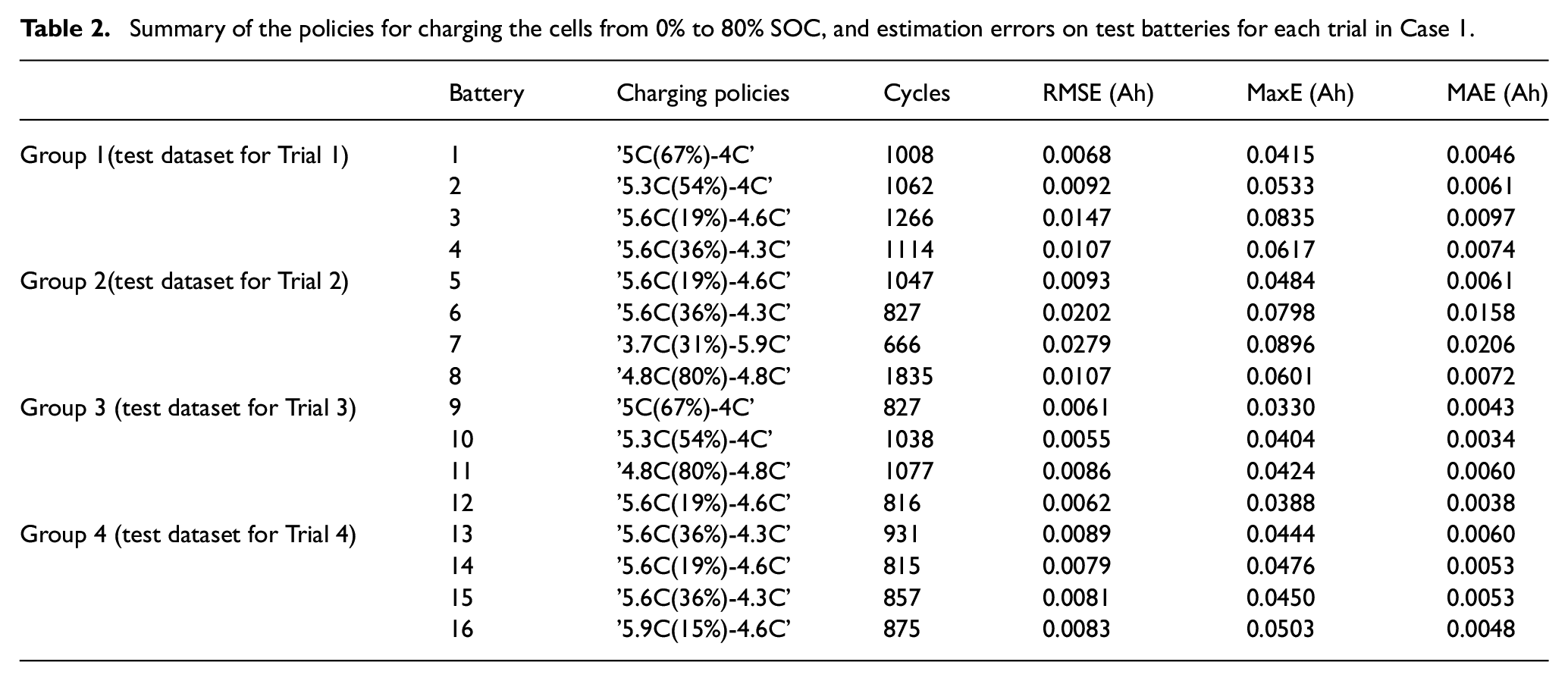
In this work, data of the first 16 batteries in dataset ‘batch3’ are used. These 16 batteries are divided into four groups, each group contains four different batteries. The detailed policies applied to charging these 16 cells from 0% to 80% SOC are summarized in Table 2, and the test cells in each trial are given in details. Each trial, samples generated from three of the four groups are first shuffled and randomly split into a training set and a validation set with the ratio of 7:3, which are then used to train the CNN model. The remaining group is finally used for testing the performance of the trained CNN model.
Summary of the policies for charging the cells from 0% to 80% SOC, and estimation errors on test batteries for each trial in Case 1.
The size of one sample inputted to the CNN is
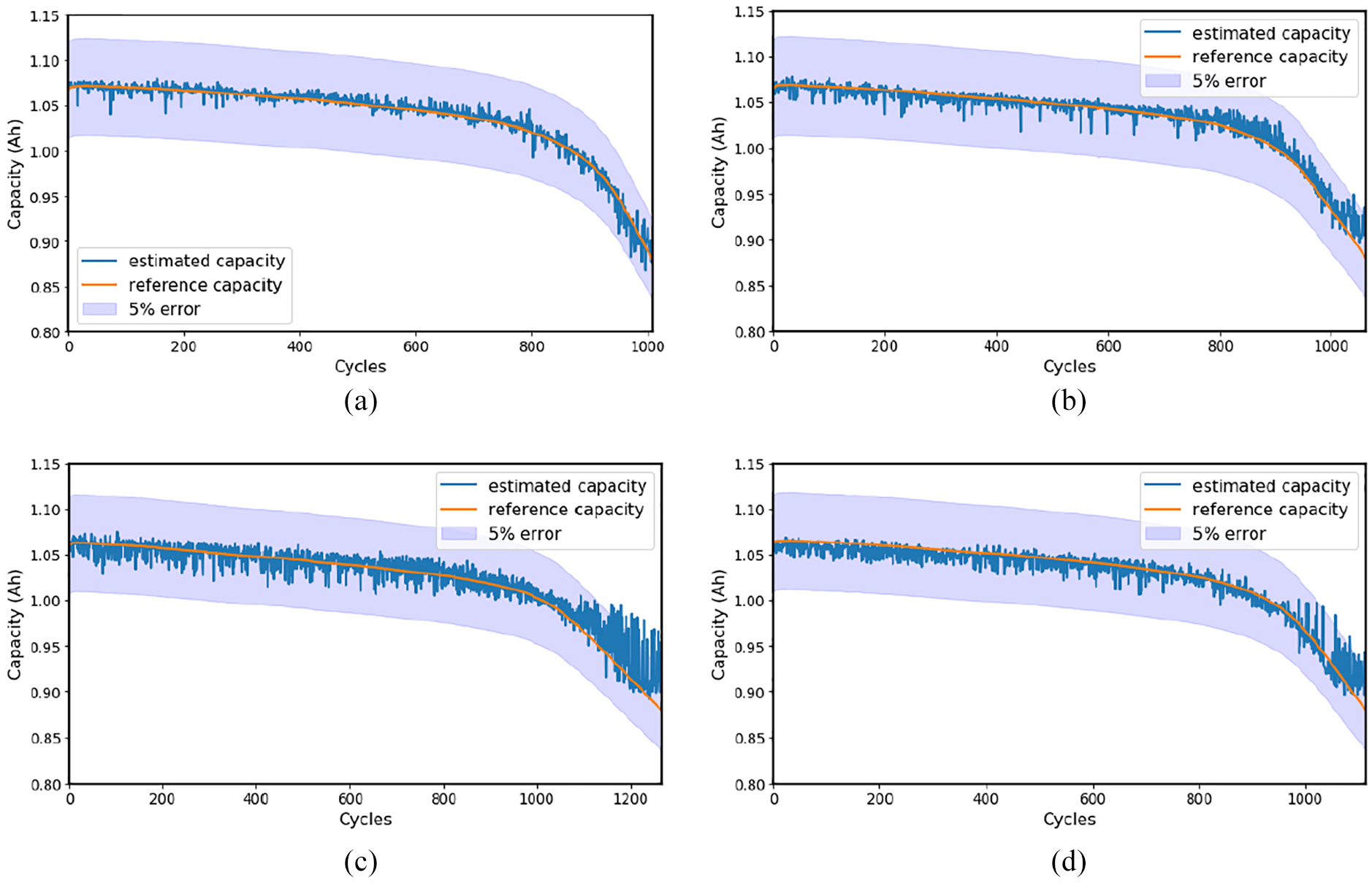
Capacity estimation results on Group 1 (Group 2, 3, 4 for training, and Group 1 for testing).
Capacity estimation results on Group 2 (Group 1, 3, 4 for training, and Group 2 for testing).
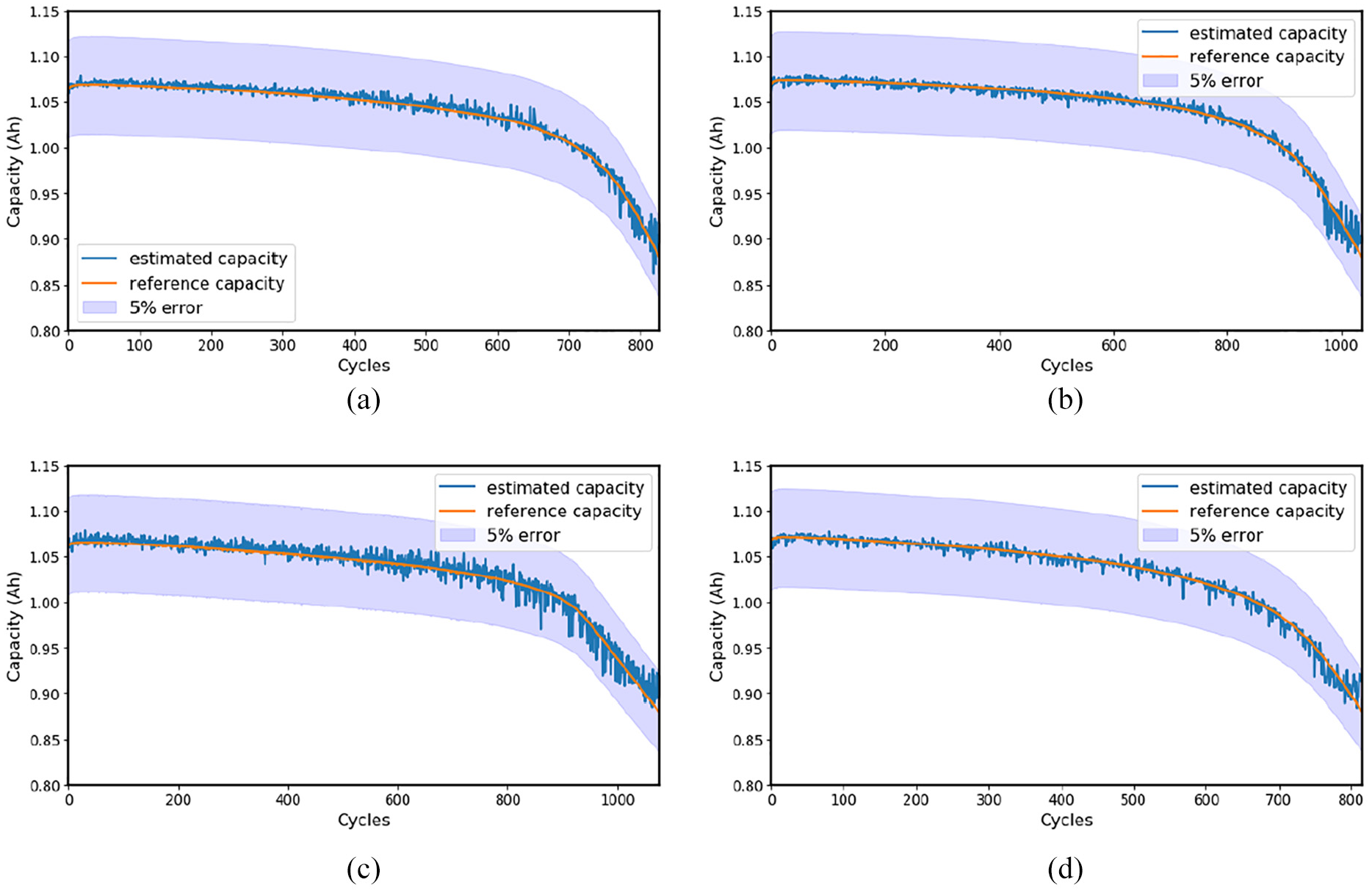
Capacity estimation results on Group 3 (Group 1, 2, 4 for training, and Group 3 for testing).
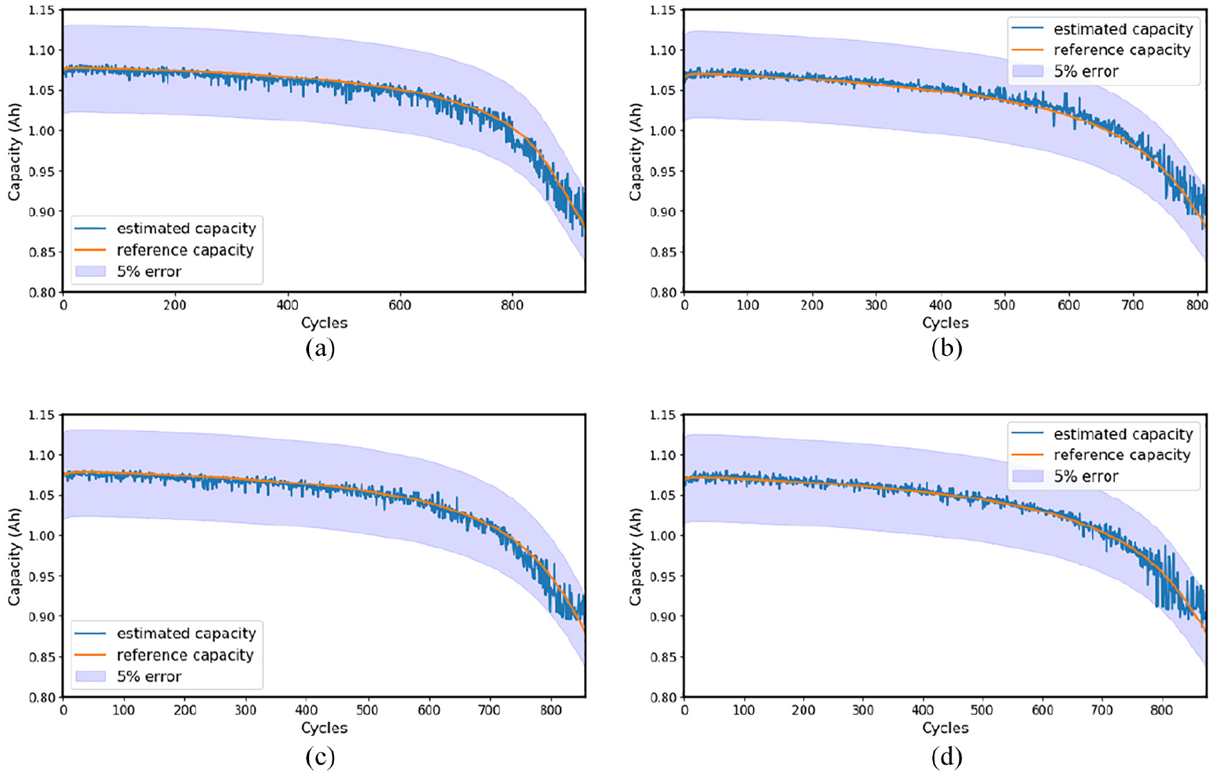
Capacity estimation results on Group 4 (Group 1, 2, 3 for training, and Group 4 for testing).
Case 2: Oxford dataset
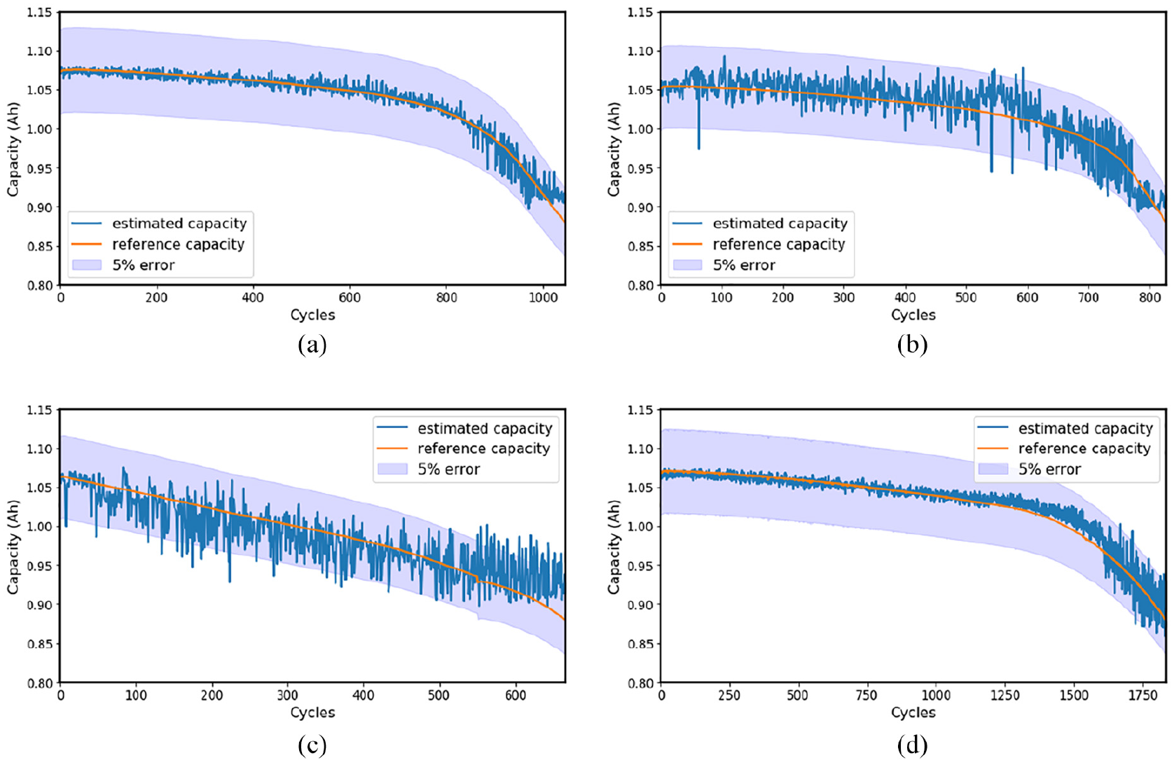
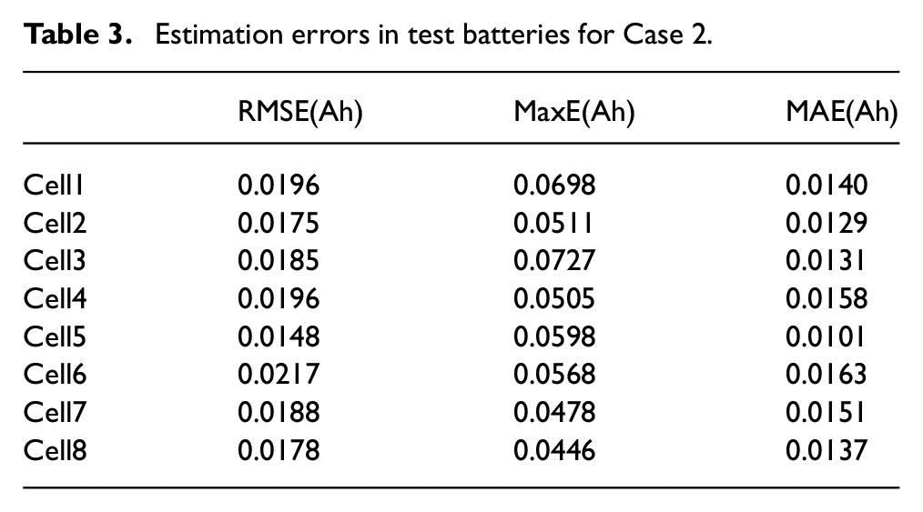
In this dataset, aging experiments are applied to eight commercial Kokam pouch cells, with a nominal capacity of 0.74 Ah. The dynamic driving profile used to degrade these cells is the Artemix urban drive cycle, and a characterization cycle is carried out every 100 dynamic cycles. The data collected from the characterization cycles, which charge and discharge the cells under a CC profile (1C) and the thermal chamber is set at a constant temperature of 40°C, are used for capacity estimation (Birkl, 2017). Each time data of seven cells are used to train the model, of which the generated samples are shuffled and split into training and validation sets with the ratio of 7:3, while data from the remaining cell is used for testing. The capacity estimation procedure in this case is the same as in case 1. The whole training and testing procedures are executed 100 times, the best estimation results on the testing dataset out of the 100 runs are shown in Figure 9, and the related RMSE, MaxE and MAE are summarized in Table 3. The RMSE is less than 0.0217 Ah, which is 2.93% of the rated capacity.
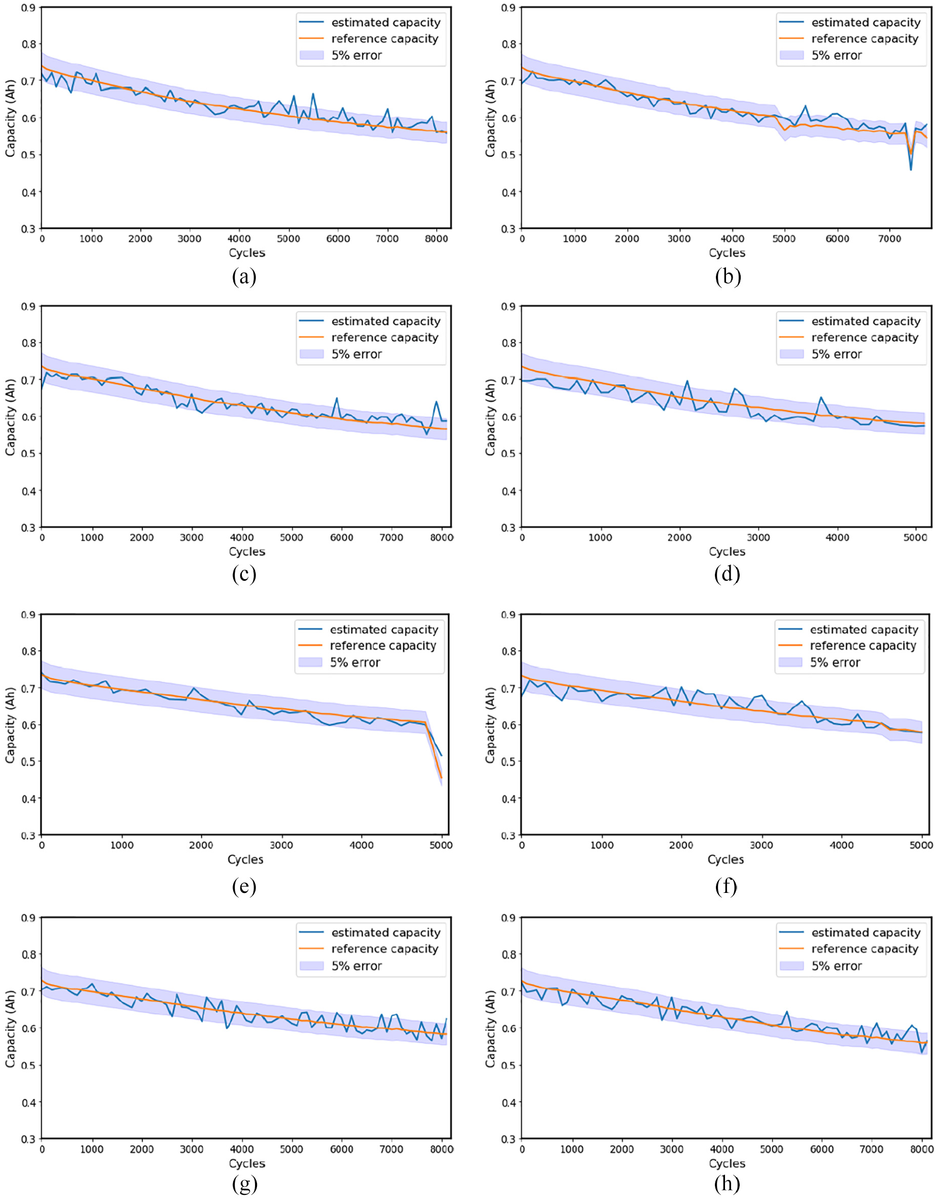
Capacity estimation results of Cell1 to Cell8.
Estimation errors in test batteries for Case 2.
Analysis
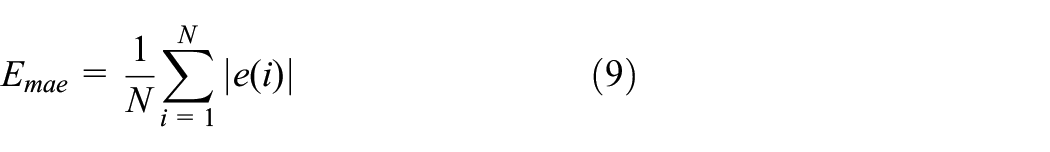
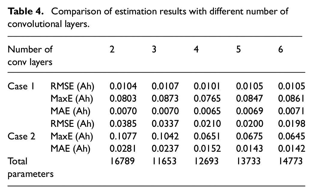
To investigate the performance of the CNN model with different number of convolutional layers in both cases, the identical training and testing datasets are used for all tests. The training and testing procedures are executed 100 times for each CNN configuration, and the average RMSE, MaxE and MAE of 100 runs are summarized in Table 4. Further, Figure 10 shows RMSE bar charts for different CNN models. It is revealed that the CNN model with two convolutional layers can achieve satisfactory results in Case 1, while four convolutional layers are required in Case 2. This is because Case 2 has less samples for training, therefore requires deeper architecture than Case 1 to extract more detailed information from limited training samples. Comparing the results of networks with four, five and six convolutional layers, and considering the total number of parameters involved in each configuration (as shown in Table 4), the CNN with four convolutional layers is the best trade-off, which can achieve satisfactory estimation results with relatively fewer parameters.
Comparison of estimation results with different number of convolutional layers.
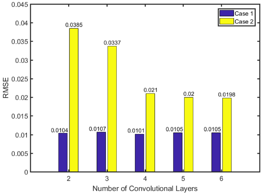
Estimation RMSE (Ah) on test datasets versus the number of convolutional layers.
In this paper, the length of consecutive data points cut from the charging and discharging curves is chosen to be 225 for each variable, and the three data chunks for current, voltage and temperature are fused to generate a
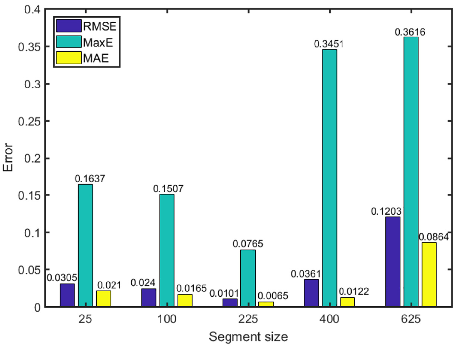
Estimation error on test datasets versus the length of segment.
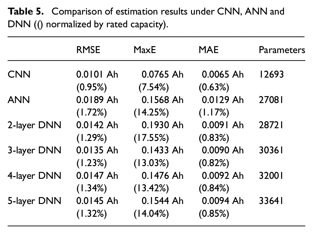
Further, Table 5 compares the capacity estimation results of CNN, ANN and DNN (with different number of hidden layers and each layer has 40 neurons) using average RMSE, MaxE and MAE of 100 runs in Case 1, and the error ratio against the rated capacity are given in parenthesis. It is obvious that the CNN model has achieved the best results while involving much less parameters.
Comparison of estimation results under CNN, ANN and DNN (() normalized by rated capacity).
In summary, the normalized RMSEs are less than 2.54% and 2.93%, respectively, on the two datasets, outperforming other machine-learning-based estimation methods.
Conclusions
This paper has proposed a novel CNN-based battery capacity estimation method only using partial charging segment of the direct measurements (e.g. current, voltage, and cell surface temperature). Compared to other ML-based methods, the proposed method is easy to implement, and can achieve fast online capacity estimation without extra health features extraction or cumulative charge calculation processes, while only raw data of a partial charging process is required. The CNN has demonstrated the capability of handling a massive amount of data to learn representative features, and the feature extraction and capacity estimation are automatically executed in one framework. To apply CNN for capacity estimation using measurable variables, a transformation method is developed to convert the time series to image representations that are acceptable by CNNs, and the converted 3-D images embed the spatially and temporally correlated information among these variables. The data segmentation method performed priori to the transformation stage not only increases the sample numbers, but also makes it possible to achieve fast online capacity estimation only using partial charging segment of direct measurements with flexible starting point. The proposed method is evaluated on two battery degradation datasets, the estimation results confirm that the proposed CNN-based method can achieve satisfactory results and can be used for fast online capacity estimation once the model is properly trained offline. The CNN model developed in this paper has a large number of parameters to tune, and to reduce the size and number of tunable parameters in the CNN model will be our future work.
Footnotes
Acknowledgements
Yihuan Li would like to thank the China Scholarship Council for sponsoring her research.
Declaration of conflicting interests
The author(s) declared no potential conflicts of interest with respect to the research, authorship, and/or publication of this article.
Funding
The author(s) disclosed receipt of the following financial support for the research, authorship, and/or publication of this article: The work is partially funded by EPSRC under grant EP/R030243/1.