
Abstract
Previous studies have shown many instances where nonprobability surveys were not as accurate as probability surveys. However, because of their cost advantages, nonprobability surveys are widely used, and there is much debate over the appropriate settings for their use. To contribute to this debate, we evaluate the accuracy of nonprobability surveys by investigating the common claim that estimates of relationships are more robust to sample bias than means or proportions. We compare demographic, attitudinal, and behavioral variables across eight German probability and nonprobability surveys with demographic and political benchmarks from the microcensus and a high-quality, face-to-face survey. In the analyses, we compare three types of statistical inference: univariate estimates, bivariate Pearson’s r coefficients, and 24 different multiple regression models. The results indicate that in univariate comparisons, nonprobability surveys were clearly less accurate than probability surveys when compared with the population benchmarks. These differences in accuracy were smaller in the bivariate and the multivariate comparisons across surveys. In addition, the outcome of those comparisons largely depended on the variables included in the estimation. The observed sample differences are remarkable when considering that three nonprobability surveys were drawn from the same online panel. Adjusting the nonprobability surveys somewhat improved their accuracy.
Keywords
Probability surveys are considered the gold standard in social science survey research, as the alternative—nonprobability surveys—often cover only a small and possibly very selective subset of the population. In contrast to probability surveys, the probability of selection into a nonprobability survey sample is unknown—and sometimes even zero—for units or subgroups of the population. Nonetheless, with the advancement of the Internet, nonprobability surveys have become easier to conduct, and their use has increased rapidly despite lacking the theoretical basis to ensure unbiased results (Baker et al. 2013). Online nonprobability surveys are often conducted using an online access panel, in which respondents self-select to answer surveys regularly (Baker et al. 2010; Callegaro, Baker, et al. 2014; McPhee et al. 2022).
Analyses using nonprobability surveys can be similarly accurate to those using probability surveys when three assumptions are fulfilled (Baker et al. 2013; Mercer et al. 2017; see also Kohler 2019). These three assumptions are often termed “ignorability,”“positivity,” and “composition” (Cornesse et al. 2020; Elliott and Valliant 2017; Mercer et al. 2017; Rosenbaum and Rubin 1983). Ignorability is fulfilled when the mechanism by which subjects are selected for the survey is independent of the variables of interest, “either unconditionally or conditional upon observed covariates” (Mercer et al. 2017:253). Positivity means that all subgroups defined by confounding variables must be represented in the survey. To generalize the results measured in a survey to the population of interest, it is also important the third assumption is met—namely, that the composition of individuals within the survey matches that of the population (Mercer et al. 2017). However, these assumptions are hard to test, and if they are not fulfilled, the results obtained from a nonprobability survey could be dramatically biased, without the researcher knowing by how much and in which direction.
One established method of investigating whether (self-)selection into nonprobability surveys can be ignorable is to compare these surveys with gold standard probability surveys or population benchmarks. Extensive empirical research using this approach indicates that nonprobability surveys produce high bias in univariate estimates (e.g., Brüggen, van den Brakel, and Krosnick 2016; Chang and Krosnick 2009; Gittelman et al. 2015; Kennedy et al. 2016; Lehdonvirta et al. 2020; MacInnis et al. 2018; Malhotra and Krosnick 2007; Yeager et al. 2011). Comparing relationships between variables within nonprobability surveys, researchers have found less bias than in univariate distributions (Berrens et al. 2003; Dassonneville et al. 2018; Kennedy et al. 2016; Pasek 2016; Stephenson and Crête 2011). The finding of lower bias is especially true for multivariate relationships (Ansolabehere and Schaffner 2014; Chang and Krosnick 2009; Dassonneville et al. 2018; Legleye et al. 2018; Pasek 2016; Simmons and Bobo 2015; Stephenson and Crête 2011). However, whereas the analyses regarding the accuracy of univariate comparisons are extensive and possibly conclusive, researchers have not yet conducted systematic tests for bivariate and multivariate relationships, and prior work includes only a few selected models. Furthermore, the existing literature on bivariate and multivariate comparisons has compared only a small number of nonprobability surveys with a few probability surveys and rarely with population benchmarks.
Researchers have suggested weighting methods to correct for the bias of nonprobability surveys compared with probability surveys or population benchmarks. As design weights are common only for probability surveys, adjustment weights are the only method to correct nonprobability surveys for possible bias, such as bias due to coverage, sampling, and nonresponse (Callegaro, Lozar Manfreda, and Vehovar 2015:183). However, the success of adjustment weighting depends on a model and is therefore not guaranteed (Vehovar, Toepel, and Steinmetz 2016:336).
Against this background, our exploratory article addresses the following four research questions:
RQ1: Do nonprobability surveys produce similarly accurate univariate estimates to probability surveys when compared with population benchmarks?
RQ2: Are nonprobability surveys similarly accurate to probability surveys in estimating bivariate and multivariate relationships when compared with population benchmarks?
RQ3: Are some univariate estimates, bivariate relationships, or coefficients of multivariate models more prone to error in nonprobability surveys than in probability surveys?
RQ4: Does weighting improve the accuracy of univariate, bivariate, or multivariate estimates of nonprobability surveys, as compared to the raw data?
We address these questions by examining all three types of analyses (univariate, bivariate, and multivariate) performed in quantitative social science research. We compare eight surveys—three probability surveys (the German General Social Survey [GGSS], the GESIS Panel, and the German Internet Panel [GIP]) and five online nonprobability surveys (designated here as NP1, NP2, NP3, NP4, and NP5)—with German population benchmarks. Additionally, we investigate the variation across different types of variables: basic demographics, occupational demographics, and substantive variables.
Previous Research Comparing Probability and Nonprobability Surveys
General Overview
Research on the usefulness of nonprobability surveys for the social sciences has increased recently. This work has considered, in particular, the bias in univariate estimation. The use of nonprobability surveys for relationships has also received attention, although most studies include only selective analyses. Table A.1 in the online supplement provides an overview of the recent research and methods used for univariate, bivariate, and multivariate comparisons between probability and nonprobability surveys. For a broad overview of the state of research, see Callegaro, Villar, et al. (2014) and Cornesse et al. (2020).
Most studies show that nonprobability surveys produce a high bias in univariate estimation (e.g., Brüggen et al. 2016; Chang and Krosnick 2009; Craig et al. 2013; Dassonneville et al. 2018; Erens et al. 2014; Gittelman et al. 2015; Kennedy et al. 2016; Lavrakas et al. 2022; Legleye et al. 2018; Lehdonvirta et al. 2020; MacInnis et al. 2018; Malhotra and Krosnick 2007; Scherpenzeel and Bethlehem 2010; Schnell and Klingwort 2023; Stephenson and Crête 2011; Yeager et al. 2011). This bias is especially prevalent concerning election results, where predictions are sometimes remarkably inaccurate (e.g., Shirani-Mehr et al. 2018; Sohlberg, Gilljam, and Martinsson 2017; Sturgis et al. 2016, 2018).
Yeager et al.’s (2011) comparative research on univariate estimates is particularly noteworthy because they compared seven nonprobability surveys with probability surveys and benchmark data. They found the nonprobability surveys produced higher bias than the probability surveys. However, they focused mainly on demographic variables. Gittelman et al. (2015) used a similar approach, comparing 17 nonprobability surveys with benchmark data, and reached comparable conclusions. Gittelman et al. (2015) also investigated using quotas to balance nonprobability samples to resemble probability samples. They found that nondemographic quotas worked best, and the complexity of the quota—that is, the number of variables or crossing them—had little effect on the accuracy of univariate estimates.
Most researchers in the social sciences are interested in going beyond univariate analyses by investigating how specific constructs are related. Comparing bivariate correlations across nonprobability and probability surveys, some researchers found less bias in nonprobability surveys than for univariate analyses (e.g., Berrens et al. 2003; Dassonneville et al. 2018; Pasek 2016; Stephenson and Crête 2011). However, other studies still found substantial differences between nonprobability and probability surveys in correlation analyses (Brüggen et al. 2016; Dutwin and Buskirk 2017; Malhotra and Krosnick 2007; Pasek and Krosnick 2020; Pekari et al. 2022). Most studies use only a small number of nonprobability surveys for bivariate comparisons (e.g., Berrens et al. 2003; Dassonneville et al. 2018; Stephenson and Crête 2011), but Brüggen et al. (2016) compared bivariate correlations across 18 nonprobability surveys and found large differences. In that study, the correlations across the nonprobability surveys differed in strength and even direction compared with a probability survey and with each other. However, these comparisons of bivariate correlations were not validated by benchmark data.
In summary, previous research is not conclusive as to whether bivariate correlations in nonprobability surveys are more accurate than univariate estimates concerning potential bias. Furthermore, there was sometimes a large variance in accuracy across nonprobability surveys when comparing the same variable pairs to probability surveys. An explanation for these mixed findings (e.g., Berrens et al. 2003; Brüggen et al. 2016; Malhotra and Krosnick 2007) could be that correlations differ in their robustness levels.
Even fewer differences might be expected between nonprobability and probability surveys in multivariate analyses than in bivariate analyses. Some researchers suggest that estimates obtained from multivariate models might be more valid for the target population (e.g., Baker et al. 2013; Jerit and Barabas 2023), especially as the models allow one to control for possible confounding effects. In practice, most comparative research on this topic seems to support the expectation of small differences (Ansolabehere and Schaffner 2014; Chang and Krosnick 2009; Dassonneville et al. 2018; Legleye et al. 2018; Pasek 2016; Simmons and Bobo 2015; Stephenson and Crête 2011). However, some studies found considerable bias in nonprobability surveys, even in multivariate analyses (e.g., Kennedy et al. 2016; Pasek and Krosnick 2020), and other work shows mixed results (e.g., Zack, Kennedy, and Long 2019).
Although most evidence points to a small bias in nonprobability surveys regarding multivariate relationships, three issues that are also problematic in bivariate analyses should be acknowledged when summarizing the previous research. First, many studies on multivariate comparisons with nonprobability surveys compared these surveys with only one probability survey without being able to evaluate the accuracy of that survey (Chang and Krosnick 2009; Pasek 2016; Pasek and Krosnick 2020; Stephenson and Crête 2011; Zack et al. 2019). Second, most studies that include multivariate models compare only a few surveys (Dassonneville et al. 2018; Pasek 2016; Pasek and Krosnick 2020; Simmons and Bobo 2015; Stephenson and Crête 2011). Therefore, it is impossible to say whether the findings of similarity are specific to these few surveys or whether nonprobability surveys, in general, are less prone to bias in multivariate than bivariate or univariate estimates. Third, most studies compare only a few models, many of which are only in political research.
Kennedy et al.’s (2016) study is a notable exception because they compared nine nonprobability surveys and one probability survey with benchmark data. For their multivariate comparison, they used four different regression models with nine independent demographic variables in each model. Two of the nine nonprobability surveys showed more correct classifications than the probability survey, suggesting that nonprobability surveys do not necessarily perform worse than probability surveys in multivariate comparisons but that this strongly depends on the specific survey.
The previous studies also allow us to summarize whether the overall nonprobability bias is different across variable types. Most studies report lower univariate bias for demographic variables than for secondary demographic variables and nondemographics (Chang and Krosnick 2009; Gittelman et al. 2015; MacInnis et al. 2018; Malhotra and Krosnick 2007; Yeager et al. 2011), especially after applying weights. However, not all prior findings are consistent. For example, Brüggen et al. (2016) found that estimates of secondary demographics (i.e., intermediate occupational education and working full-time) were, on average, more biased than estimates of substantive variables (i.e., having good health and being satisfied with life). Lavrakas et al. (2022) found the opposite when comparing a similar set of variables. Of the demographic variables, education consistently showed biased estimates (Malhotra and Krosnick 2007; Mercer and Lau 2023; Yeager et al. 2011), and of the secondary demographics, employment status (Brüggen et al. 2016; Gittelman et al. 2015; Lavrakas et al. 2022), religious affiliation (Gittelman et al. 2015), Internet access at home, having dependent children, and speaking other languages (Lavrakas et al. 2022) were strongly biased. Concerning substantive variables, many researchers found estimates of political variables, such as vote choice, turnout, and party identification, to be especially biased (Chang and Krosnick 2009; Kennedy et al. 2016; Malhotra and Krosnick 2007; Scherpenzeel and Bethlehem 2010), whereas other work (e.g., Dassonneville et al. 2018; Mercer and Lau 2023) found estimates of political variables to be less biased than secondary demographics.
With respect to bias in correlations of individual variables, most studies only report the bias for a small number of selected correlations. Pasek and Krosnick (2020) provide a broad overview of bivariate associations, which suggest the correlations between demographic variables are more prone to sample differences than those between substantive variables (for similar results, see Pekari et al. 2022). Regarding multivariate models, Simmons and Bobo (2015) found that the effect of education on egalitarianism and racial resentment differs across probability and nonprobability surveys.
Overall, for all three comparison types—univariate, bivariate, and multivariate comparisons—prior research has found that demographic variables often have higher nonprobability bias than substantive variables. A possible reason for this finding could be that demographic variables are more strongly associated with participation in nonprobability surveys than are substantive variables.
One common factor of all the relevant studies (see Table A.1 in the online supplement) is that the compared nonprobability surveys were exclusively conducted online. However, probability surveys have been found to be more accurate than nonprobability surveys independent of the mode of data collection; researchers have compared online nonprobability surveys with probability surveys conducted face-to-face (e.g., Brüggen et al. 2016; Dassonneville et al. 2018; Malhotra and Krosnick 2007; Simmons and Bobo 2015), online (e.g., Kennedy et al. 2016; MacInnis et al. 2018; Yeager et al. 2011), and via telephone (e.g., Lavrakas et al. 2022; Pasek and Krosnick 2020; Yeager et al. 2011). Notably, probability surveys were still found to be more accurate in univariate estimation, even when the probability surveys had a low response rate—for example, around 20 (Gittelman et al. 2015; Pasek and Krosnick 2020) or 15 percent (e.g., Lavrakas et al. 2022; MacInnis et al. 2018).
Most of these studies include some method of weighting to adjust nonprobability and probability survey data and correct for sampling bias. Although Wang et al. (2015) found that adjusted nonprobability surveys could be similarly accurate to probability surveys, most studies find little improvement in accuracy when the data are weighted (e.g., Chang and Krosnick 2009; MacInnis et al. 2018; Pasek and Krosnick 2020). In some cases, weighting even increases bias instead of reducing it (Brüggen et al. 2016; Yeager et al. 2011). Echoing previous findings, recent studies by Lavrakas et al. (2022) and Kocar and Baffour (2023) found that weighting was more successful for probability than for nonprobability surveys, especially concerning demographic variables.
Previous Analysis Methods for Survey Comparisons
Because the comparison of the accuracy of univariate estimates of nonprobability and probability surveys has been well-researched over the years, researchers have established several analysis methods (for an overview, see Callegaro, Villar, et al. 2014; MacInnis et al. 2018). The most common methods include the mean of variables in different surveys (e.g., Dassonneville et al. 2018; Stephenson and Crête 2011), the proportion of one category (e.g., Brüggen et al. 2016; Kennedy et al. 2016; Yeager et al. 2011), and the average absolute bias over all categories of a single variable between the survey and a benchmark (e.g., Ansolabehere and Schaffner 2014; Chang and Krosnick 2009; Sturgis et al. 2016). In addition, Dassonneville et al. (2018) used a Kolmogorov–Smirnov test to evaluate the similarity in distributions. Table A.1, column 2, in the online supplement provides an overview of the methods typically used.
The methods above can evaluate only the accuracy of individual variables. To compare the overall accuracy between surveys, some researchers use the average error across all variables of interest (e.g., Ansolabehere and Schaffner 2014; Dutwin and Buskirk 2017; Kennedy et al. 2016; Yeager et al. 2011), and MacInnis et al. (2018) use the root mean square error (RMSE), in which the error of every variable is first squared, then averaged, and then the square root of the measure is taken. Therefore, variables with more errors have a bigger effect on the RMSE as compared to the average absolute error.
For bivariate estimates, two methods dominate the literature comparing relationships between probability and nonprobability surveys. First, some studies compare correlation matrices with all pairs of variables (Pak, Cotter, and Thorson 2022; Pasek and Krosnick 2020). The second method fits separate bivariate regression models for specific variable combinations, and an interaction term is used to indicate the differences between the surveys (e.g., Brüggen et al. 2016).
Applying the first method, Pasek and Krosnick (2020) use the difference in Pearson’s r, comparing one probability survey and one nonprobability survey over several weeks. Pak et al. (2022) visualize the differences using a heatmap of correlation matrices. Using a simpler method based on cross-tabulating the data, Dutwin and Buskirk (2017) compare the difference between every table cell in the survey and the same cell in the benchmark data and then calculate the average bias for the survey from these cell differences (for a similar approach, see Pekari et al. 2022). Using the latter method, Brüggen et al. (2016) compare different bivariate regression models to evaluate the effect of age, gender, and health on life satisfaction (see also Dassonneville et al. 2018; Malhotra and Krosnick 2007). The results achieved with this method can provide an excellent overview of the bivariate bias, but they are either bound to a small or moderate number of variables with a limited number of categories or the number of cells can be overwhelming. Also, the method can be problematic for small samples because there might be empty cells.
For multivariate comparisons, prior work has used different kinds of regression models. Some researchers compare the results of multivariate ordinary least squares regressions (e.g., Simmons and Bobo 2015), others compare logistic or ordinal regression results (e.g., Ansolabehere and Schaffner 2014; Kennedy et al. 2016; Zack et al. 2019), and one study used different regressions depending on the variable of interest (Chang and Krosnick 2009). For the regressions, these researchers either use separate models and compare the coefficients (e.g., Ansolabehere and Schaffner 2014) or use a single model and include an interaction term, indicating the different surveys (e.g., Dassonneville et al. 2018). For logistic regressions, researchers compare regression coefficients (e.g., Ansolabehere and Schaffner 2014) or marginal effects (e.g., Zack et al. 2019).
Research Methodology
Data
For this study, we used eight surveys: three probability surveys (the GGSS, the GESIS Panel, and the GIP) and five nonprobability (NP) surveys (NP1, NP2, NP3, NP4, and NP5). As population benchmarks, we used variables from the German microcensus. Because the surveys were not originally conducted for this comparison, not every survey had the same questionnaire and included the same variables. In NP1, the target population comprised respondents aged 20 years or older. To ensure comparability, we excluded respondents younger than 20 years from the other surveys. As all nonprobability surveys were conducted online, we chose to operationalize the comparison by only including online modes of probability surveys if possible (GESIS Panel and GIP). For the GGSS and the microcensus, which were conducted face-to-face, we utilized a measure indicating Internet usage to exclude non-Internet users.
Overall, the number of missing values was relatively low, with some notable variation across variables and datasets (see Table C.11 in the online supplement). To keep all available information and to minimize the information loss for each analysis, we excluded cases with missing information only if absolutely necessary. For the univariate estimation, we excluded cases with missing information separately for each variable. In the bivariate estimation, we used pairwise deletion. In the multivariate estimation, cases with missing values were removed if at least one of the variables of each of the respective models showed missing values. This treatment of missing values resulted in sample sizes that slightly differed by the kind of analysis and variables that were involved.
In the following, we briefly introduce the surveys included in our comparison and the population benchmarks with which they are compared. Table 1 provides an overview of the surveys; a more detailed description, guided by the AAPOR (2021) disclosure standards, can be found in Part B of the online supplement.
Descriptions of the nine surveys of comparison.
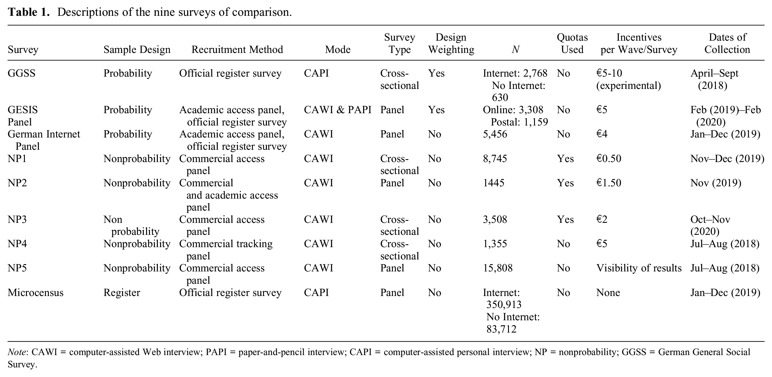
Note: CAWI = computer-assisted Web interview; PAPI = paper-and-pencil interview; CAPI = computer-assisted personal interview; NP = nonprobability; GGSS = German General Social Survey.
The German General Social Survey (GGSS)
The GGSS (GESIS – Leibniz Institute for the Social Sciences 2019) is an established, cross-sectional probability survey conducted every two years. In the present comparison, we use the GGSS 2018, which was fielded between April and September 2018. In 2018, 10,731 persons in Germany were randomly selected. Of these, 3,477 participated and were interviewed face-to-face. After omitting ineligible respondents younger than age 20, 3,409 cases were included in the final dataset, of which 2,768 regularly used the Internet. To include enough respondents from Eastern Germany, the population in that region was oversampled. We use the provided design weight to correct for this oversampling.
The GESIS Panel
The GESIS Panel (GESIS – Leibniz Institute for the Social Sciences 2022; see also Bosnjak et al. 2018) is a mixed-mode, panel-based probability survey established in 2014. Between 2014 and 2020, six waves per year were conducted. The initial sampling frame for the panel was comprised of all German citizens aged 18 to 70 years. The panel consists of three cohorts, recruited in 2013, 2016, and 2018. In 2013, each person was interviewed face-to-face, and only essential, mainly demographic, questions were asked. Most respondents participated online in the panel; those who could not or were unwilling to do so could participate by postal mail. Therefore, the GESIS Panel includes both online and offline respondents. For our study, we use only information from respondents who participated in the waves for which data collection started in 2019. Consequently, the field period was February 2019 to February 2020. If questions were asked in multiple waves during the field period, we used only the most recent information. Some questions (mainly demographics) were asked in the recruitment survey and were updated only if something had changed. The sample comprised 4,711 respondents, of whom 3,472 were online respondents. To make the results comparable with the web-based nonprobability surveys in our study, we include only online respondents aged 20 years or older. The final sample includes 3,308 respondents. The GESIS Panel provides design weights, which we use in our analyses.
The German Internet Panel (GIP)
The GIP is an online, probability-based panel survey (Blom, Gathmann, and Krieger 2015). 1 It has been conducted since September 2012, with six waves per year and changing questionnaires. The panel was recruited in 2012 from the population of all German citizens aged 16 to 75 years and refreshed from the same population in 2014 and 2018. Respondents without Internet access were provided with a free Internet connection and a computer in 2012 or a tablet in 2014. For our analyses, we use respondents who participated in waves 39 to 44, fielded between January 2019 and December 2019. As some target questions were asked in 2020 or 2021 but not 2019, we also include these results for the specific variables. The number of participants in 2019 was 5,549. After removing ineligible respondents, the final sample consists of 5,456 respondents.
Nonprobability surveys
The study includes five nonprobability surveys, but they partly stem from the same nonprobability panel. NP1, NP2, and NP3 were drawn from an online panel provided by Respondi (2019), which consists of around 100,000 panel members. Panel members are recruited from several sources, including Respondi’s own opinion platforms, online marketing campaigns, and advertisements on search engines. NP4 was also provided by Respondi; however, it was gathered from a small subsample of about 2,000 online panelists who agreed to participate in web-tracking of their browser history. NP5 stems from an online panel provided by Civey, which comprises 6 million registered users and is mainly recruited via river sampling, using advertisements on German (news) websites (e.g., Der Spiegel, see Richter, Wolfram, and Weber 2022). The overlap in panel providers reduces our ability to compare different panels, but it allows us to investigate the similarity of conducting different nonprobability surveys with the same online panel.
NP1 to NP3
The first three online nonprobability surveys were conducted in November to December 2019, November 2019, and October to November 2020, respectively. Respondents were drawn from the vendor’s online access panel. For all surveys, quotas were used. For NP1, they were based on sex, region (residence in Eastern/Western Germany), marital status, and cross-tabulated age and education; NP2 and NP3 used cross-tabulated quotas based on age, sex, and education. The final sample sizes were 8,745 (NP1), 1,445 (NP2), and 3,508 (NP3). Additional information can be found in Table 1 and in Part B of the online supplement.
NP4
Respondents for the fourth online nonprobability survey, NP4, were drawn from a commercial web-tracking panel. The sampling was conducted without using quotas. Between July and August 2018, 1,734 respondents aged 18 or older were invited to participate in the cross-sectional online survey. Of these, 1,355 completed the survey. The final sample comprised 1,307 respondents.
NP5
The fifth nonprobability survey, NP5, was conducted by Civey, another commercial survey vendor, between June and August 2018. The population for this cross-sectional online survey comprised German citizens aged 18 years or older. No quotas were used. The questionnaire comprised 12 questions about two of the Big Five personality traits: conscientiousness and emotional stability (see Murray-Watters et al. 2022). The vendor’s sampling method was unique in that respondents were asked each question individually, and questions from other single-item surveys could appear in between the NP5 survey questions. The vendor provided a sample in which at least 8,874 respondents answered all 12 questions, and 15,915 respondents answered at least one of them. Thus, after removing ineligible respondents, the final sample comprised 15,808 respondents.
Population benchmarks
For the population benchmarks, we used the German microcensus 2019 scientific use file (SUF, see Research Data Center (RDC) if the Federal Statistical Offices and Statistical Offices of the Federal States, 2019). The German microcensus is a large-scale, annual register-based survey of 1 percent of the population in Germany. The SUF contains a 70 percent random sample. Although the federal survey is continually in the field, we used only the cases from 2019 for our comparison, as it was the most recently available microcensus. The survey population comprised all persons aged 15 years and older residing in private and collective households in Germany. As all eligible members of sampled households are obliged by law to answer the survey, the unit nonresponse rate was only 3.2 percent. To make the sample comparable, we excluded respondents who had not used the Internet in the three months preceding the survey. The 2019 German microcensus SUF survey comprised 596,858 persons. After omitting respondents younger than age 20 and those who had not used the Internet, the sample comprised 350,913 respondents.
For the multivariate analyses, we could not use the microcensus as a benchmark survey due to data protection requirements. Thus, we used the weighted GGSS as a benchmark survey instead. We also used the GGSS as a benchmark survey for univariate and bivariate comparisons that included political variables and religious affiliation, as these variables were not collected in the microcensus.
Variables Included in the Comparison
The present study compares (a) basic demographic variables—namely age, education, marital status, region, sex, personal income, and household income; (b) occupational demographic variables related to vocational education and training (vocational training) and employment status; (c) a range of variables measuring political attitudes and behaviors—namely, political interest, left–right self-placement, satisfaction with democracy, political efficacy (internal and external), voting intention, and trust in German institutions (parliament, government, the courts, the police); and (d) religious affiliation (see Table 2 for an overview).
Variables Used for the Survey Comparisons.
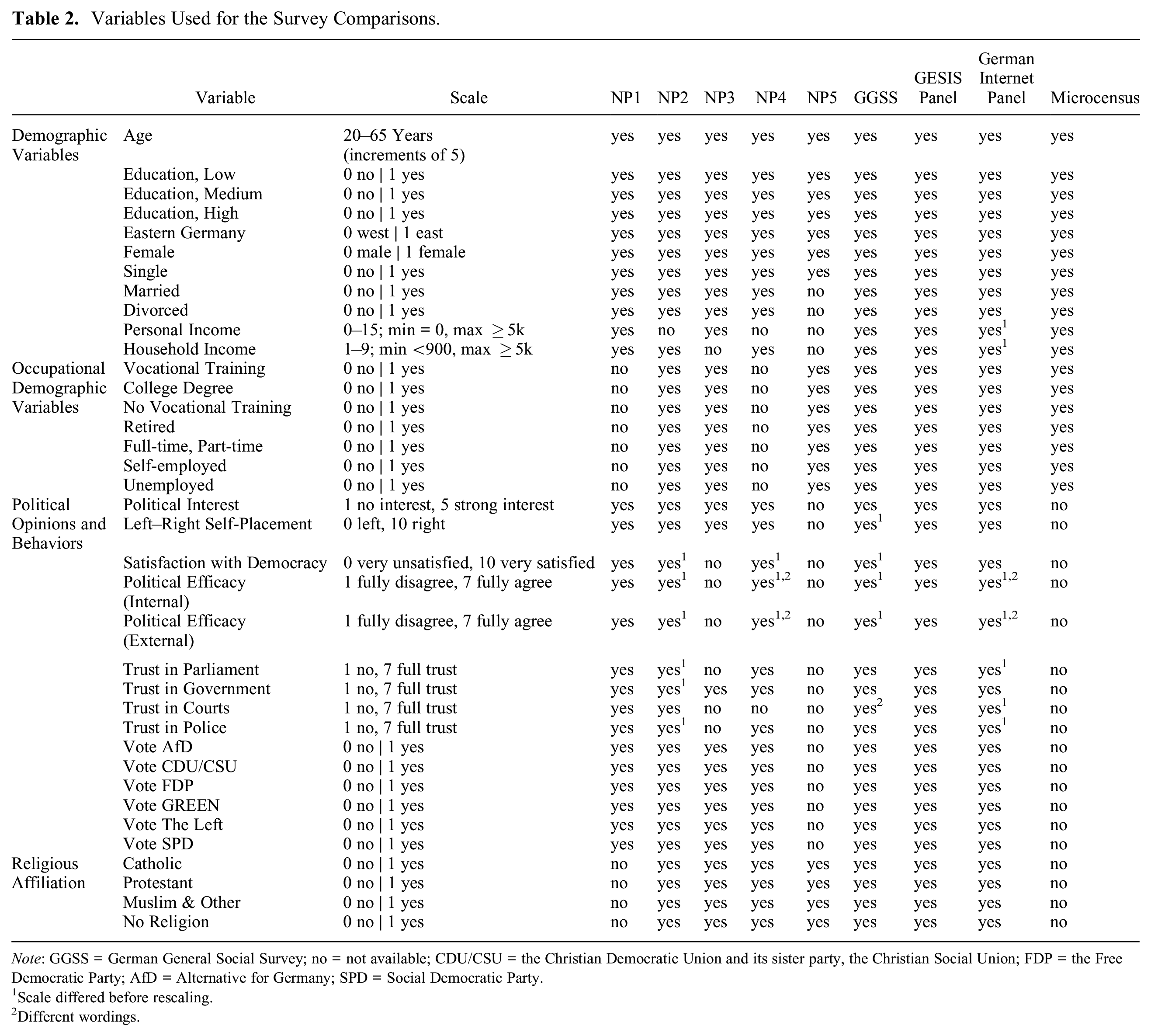
Note: GGSS = German General Social Survey; no = not available; CDU/CSU = the Christian Democratic Union and its sister party, the Christian Social Union; FDP = the Free Democratic Party; AfD = Alternative for Germany; SPD = Social Democratic Party.
Scale differed before rescaling.
Different wordings.
Not every variable was available in every survey, so we limited the comparisons to the available variables. The measurement of political variables might be time-sensitive (e.g., voting intention, left–right self-placement, trust in institutions), as the political climate can change rather quickly. Therefore, given the different field periods of the surveys (see Table 1), we expected larger heterogeneity across surveys for political measures. In contrast, other variables, such as personal income, might be time-sensitive on an individual level but more robust on an aggregated level, as investigated in our comparisons.
Analytic Plan
Univariate Analyses
In the univariate analyses, we used the absolute bias.2,3 In addition to this measure, we evaluated how the distribution of the variables differed. To do so, we used a chi-square goodness-of-fit test 4 to compare the variables across surveys (see Tables C.1 and C.2 in the online supplement). To assess the overall accuracy of a survey concerning benchmark data, we used the RMSE as suggested by MacInnis et al. (2018). Confidence intervals were Bonferroni adjusted, using the number of variables (4 to 19, depending on survey and analyses) as the number of comparisons.
Bivariate Analyses
For the bivariate analyses, we compared the correlation matrices of the surveys. In this comparison, we measured the correlation of every variable used in the univariate analyses with every other variable. As in the case of univariate analyses, benchmarks for correlations were taken from the microcensus and the GGSS.
The evaluation proceeded in two steps. First, using the selected variables, we fitted a correlation matrix for the microcensus and the respective surveys. Categorical variables consisting of fewer than four categories (e.g., education) were transformed into dummy variables. We estimated the correlation of every variable with every other variable using Pearson’s r. 5 Second, we used bootstrapped p-values (Thulin 2021) to examine whether a correlation in the respective matrix differed significantly from that estimated with the benchmark survey. In addition to the significance tests, we considered a correlation to be substantially different only if at least one of the estimated correlations differed significantly from zero. Otherwise, one would still arrive at the same substantive interpretation using either survey—namely that the correlation is nonsignificant. If a difference was statistically significant, we distinguished between two levels of difference: small and large. We classified a statistically significant difference as large if the correlation measured with one survey was at least double the size of that measured with the other, or if the correlations measured with each survey differed in direction. In all other cases, the difference was considered to be small. We accounted for the problem of multiple comparisons by using Bonferroni adjustments (see Shaffer 1995); the number of comparisons was assumed to be the number of variables in every comparison (11 to 37 depending on survey and analyses).
Multivariate Analyses
To compare estimates from multivariate analyses, we used two types of regression models, depending on the data type. Specifically, we used ordinary least squares (OLS) regression models 6 for quasi-metric dependent variables 7 and binary logistic regressions 8 for dichotomous dependent variables. Similar to the bivariate analysis, we started by estimating the same models for the surveys of comparison and the benchmark survey and followed by using bootstrap p-values of the differences of estimates to assess whether the coefficients of the compared surveys were significantly different from another. If a regression coefficient was statistically significant and the coefficient was significant in at least one of the surveys, we considered the respective relationship to differ between the surveys. As in the bivariate analysis, we distinguished between small and large differences by categorizing a difference as large when the effect in one sample was double the size of the comparison survey’s effect, or if the coefficients differed in direction.
We used Bonferroni adjustment and robust standard errors, and we show a plot with a color scheme distinguishing between small and large differences. For the Bonferroni adjustment, we assumed the number of comparisons to be equal to the number of models compared (7 to 24 depending on the survey). To keep the multivariate regression models simple and comparable, we used the same independent variables for every model because results may depend on the combination of predictors (see Malhotra and Krosnick 2007), and adding predictors is not always beneficial as they might introduce additional error (see Pekari et al. 2022). Our selection approach corresponds to Kennedy et al. (2016) and Zack et al. (2019), who also used demographic variables as independent variables for several models in a multivariate comparison of probability and nonprobability surveys.
Thus, in each of the regression models, we use the same six basic demographic variables as independent variables: age, two education dummies, living in Eastern or Western Germany, sex, and being single. We selected these variables because (a) they are standard demographic variables that are included in many models, (b) they are known to be correlated with many other variables, and (c) they allow us to include several models to ensure the results are robust across models. As mentioned earlier, we could not use the microcensus as a benchmark survey in the multivariate comparison for data protection reasons.
Weighting
We weighted the data for all our main analyses. To create the weights, we used raking, a form of superpopulation modeling (McPhee et al. 2022). Raking is an iterative adjustment method that uses auxiliary data to adjust the survey composition to the marginal distributions of the population. For the raking, we used the rake function of the survey package in R, setting the maximum number of iterations to 1,000 (Lumley 2023). Two of the probability surveys provided design weights (GGSS and GESIS Panel), which we used as base weights for those surveys and integrated into the raking process. We did not receive weights from the nonprobability providers for any of the five surveys.
To calculate the adjustment weights in every survey, we used the following commonly used demographic variables: age, education, personal income, household income, sex, marital status, and living in Eastern or Western Germany (for more details on weighting for individual surveys, see Part B of the online supplement). As benchmarks for the weighting, we used data from the German microcensus. We imputed missing values for the variables used for weighting (see Table C.11 in the online supplement) using predictive mean matching (Little 1988). Finally, we compare our results to findings from unweighted data (RQ4).
Estimation of Precision
As the nonprobability surveys cannot be assumed to act as a simple random sample, using common analytic formulas to calculate the precision of estimates can be problematic. Unfortunately, there is no established approach to estimating precision for nonprobability samples (Lavrakas et al. 2022). Therefore, we follow the practice suggested by AAPOR (McPhee et al. 2022; see also Erens et al. 2014; Lavrakas et al. 2022) and use bootstrapping with 2,000 iterations in all our comparisons to calculate the confidence intervals and p-values.
We derived 95 percent confidence intervals, using the 2.5 and 97.5 percent quantiles of the resulting bootstrapped distribution of the statistics of interest as upper and lower bounds (see, e.g., Davison and Hinkley 1997). To calculate the bootstrapped p-values, we used the confidence interval inversion method (Thulin 2021). Here, the p-value is approximated as the smallest α for which the 1 –α confidence interval does not include the value of comparison. We applied weights using the survey package (Lumley 2023) in every bootstrap iteration to obtain the weighted estimates. We conducted all statistical analyses with R (R Core Team 2022; for a list of used R packages, see Part G of the online supplement).
Robustness Checks
The compared surveys contain partially different sets of variables, which could influence the assessments of average accuracy. To control for these sample differences, we performed a first set of robustness checks, including only variables that were present in all surveys in the respective comparisons (see Figures E.1.1 to E.5.2 in the online supplement). Specifically, NP1 and NP4 had very few variables in common with NP5, so we conducted robustness checks based on two sets of surveys with their respective shared set of variables, one including all surveys except NP5 and a second including all surveys except NP1 and NP4. Furthermore, as the variables used for weighting differed partially between surveys, due to different availabilities, we also conducted robustness checks using weights based on the minimal set of shared weighting variables (i.e., age, sex, education, being single or not, living in Eastern or Western Germany; see Figures F.1 to F.5 in the online supplement).
Results
Univariate Comparison
Figure 1 shows the bias in the demographic variables (for variables that were not used for weighting) compared with the microcensus benchmark survey for the weighted 9 probability surveys (left panel) and the weighted nonprobability surveys (right panel; for exact values, see Table C.3 in the online supplement). 10 The RMSE value in the panels’ top-right corner indicates a survey’s average bias. Of the compared surveys, the face-to-face survey GGSS had the lowest RMSE (0.025). NP2 (0.038), the GIP (0.046), and the GESIS Panel (0.048) had medium average biases, followed by NP5 (0.071) and NP3 (0.08) showing higher biases.

Univariate accuracy of probability and nonprobability surveys compared with the microcensus benchmarks: basic demographic variables and occupational demographic variables, Bonferroni-adjusted, weighted.
Even when the RMSEs were similar, the bias concerning individual variables sometimes varied greatly across the samples. The GESIS Panel, for example, had the smallest bias of all surveys when measuring self-employment (0.002) but had a large bias on vocational training (0.083). NP3 had the largest bias of all surveys when measuring retirement (0.142) but no bias on having a college degree (0.005). Therefore, even surveys with a small RMSE can be biased strongly on specific variables, and surveys with overall high bias can be accurate.
In addition to demographic variables, we also examined substantive variables. Figure 2 shows the results of the comparison (for exact values, see Table C.3 in the online supplement). We used the GGSS as the benchmark survey for this comparison, as the microcensus collected only demographic variables and occupational demographics. Figure 2 indicates that the GESIS Panel and the GIP had the lowest RMSE (0.039 and 0.039)—that is, they were both more like the GGSS than any of the nonprobability surveys. Of the nonprobability surveys, NP3 (0.05) was most similar to the GGSS benchmark survey, followed by NP2 (0.061), NP1 (0.072), NP4 (0.074), and NP5 (0.102). However, for NP5, only religious affiliation variables could be compared.
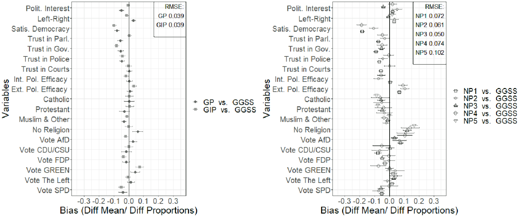
Univariate accuracy of probability and nonprobability surveys compared with the GGSS benchmarks: political variables and religious affiliation, Bonferroni-adjusted, weighted.
Summarizing the univariate results concerning RQ1—whether nonprobability surveys are similarly accurate as probability surveys on a univariate level—the nonprobability surveys were less accurate overall than the probability surveys. Furthermore, although some nonprobability surveys were relatively accurate, some showed a large bias. By contrast, the probability surveys seem more consistent regarding their overall accuracy.
Bivariate Comparison
The results of the bivariate comparisons of the demographic variables with the microcensus benchmarks are displayed in Figure 3, which shows the difference between each survey and the microcensus in the bivariate correlation estimates for each pair of variables in the univariate comparison. Pairs of variables that were not measured in a specific survey were omitted. The accuracy in percent was calculated from all correlations for all 18 variables, which led to a correlation matrix of 153 = (
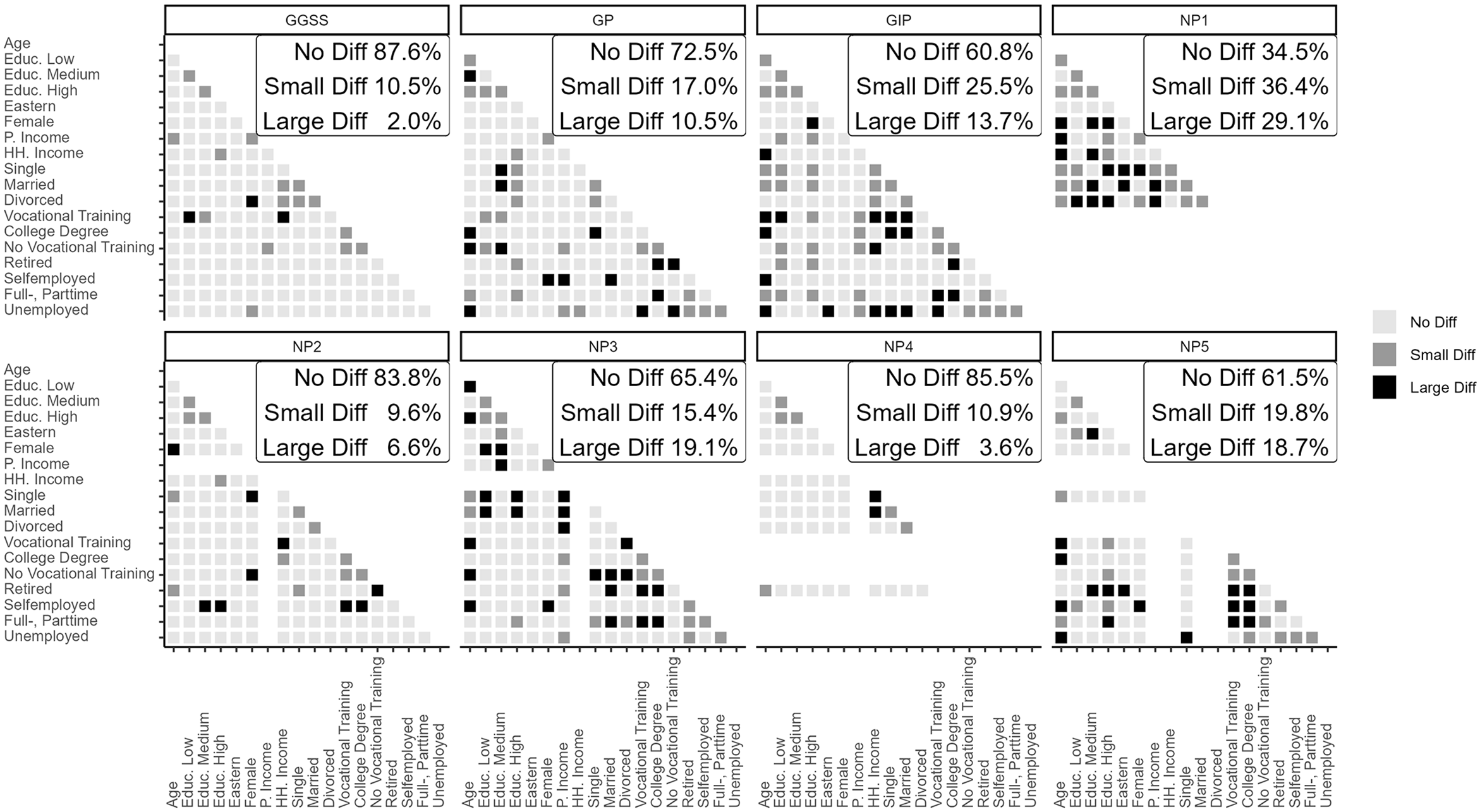
Bivariate comparison of probability and nonprobability surveys with the microcensus benchmarks: pairs of basic demographic variables and occupational demographic variables, Bonferroni-adjusted, weighted.
In summary, the probability surveys had similarities ranging from 87.6 to 60.8 percent, whereas the similarities between the nonprobability surveys and the benchmark survey ranged from 85.5 to 34.5 percent, showing a wider range of bias in bivariate estimates. On average, for the probability-based surveys, only a few demographic correlations showed a large difference (8.7 percent; see Table C.12 in the online supplement), and the average proportion of large differences was higher for the nonprobability surveys (15.4 percent). The largest part of the average differences was due to differences in magnitude (8.1 percent for the probability surveys and 14.3 percent for the nonprobability surveys).
Figure 4 expands the bivariate comparison of correlations and includes both demographic and political variables, using the GGSS as the benchmark survey. This comparison included up to 38 variables, leading to a maximum of 703 = (
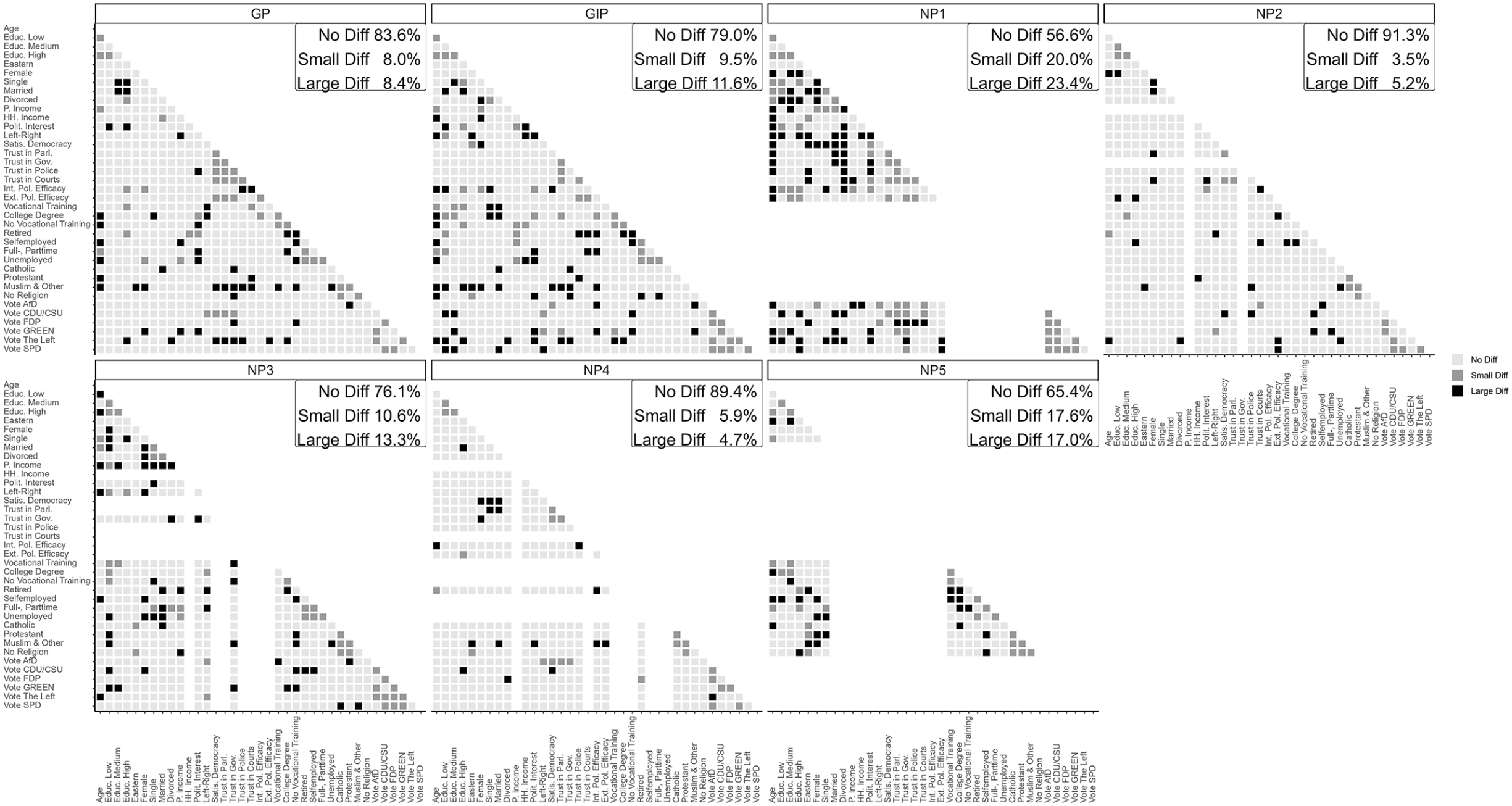
Bivariate comparison of probability and nonprobability surveys with the GGSS benchmarks: pairs of demographic variables, political variables, and religious affiliation, Bonferroni-adjusted, weighted.
The average proportion of large differences compared to the GGSS was relatively low (3.9 percent for the probability surveys and 7.5 percent for the nonprobability surveys, see Table C.13 in the online supplement). Those differences were mostly due to differences in magnitude (3.9 percent in probability surveys and 6.6 percent in nonprobability surveys). Overall, compared to the GGSS, and including additional variables, the differences between all surveys and the benchmark survey seem less pronounced than comparing the surveys to the microcensus, although the GGSS and the microcensus were very similar (only 2.0 percent large differences).
Summarizing the bivariate results regarding RQ2—whether nonprobability surveys are similarly accurate as probability surveys regarding relationship estimates—our analyses indicate that bivariate estimates of the probability surveys were remarkably similar to estimates of the benchmark survey. By contrast, for the nonprobability surveys, the results show that correlations within demographic variables were sometimes very different, and the correlations of political variables with other variables (either demographic or substantive) were more robust (see Figure C.1 in the online supplement).
Multivariate Comparison
Figure 5 shows results for the multivariate models with political and demographic variables as dependent variables, using the GGSS as the benchmark survey. In the visualization, each column represents one model with a different dependent variable, and each square is a coefficient within that model. Some surveys were similar to the GGSS (“No Diff”: NP4 96.5 percent; NP2 96.2 percent; GESIS Panel 95.1 percent; GIP 89.6 percent; NP3 88.2 percent). However, NP1 (80.4 percent “No Diff”) and NP5 (73.8 percent “No Diff”) differed somewhat more strongly. On average, a sizable proportion of the multivariate differences were large (10.0 percent of 18.8 percent for the probability surveys, 12.7 percent of 24.2 percent for the nonprobability surveys; see Table C.14 in the online supplement); as with the bivariate comparison, these are mostly differences in magnitude (8.6 percent for the probability surveys, 10.8 percent for the nonprobability surveys).
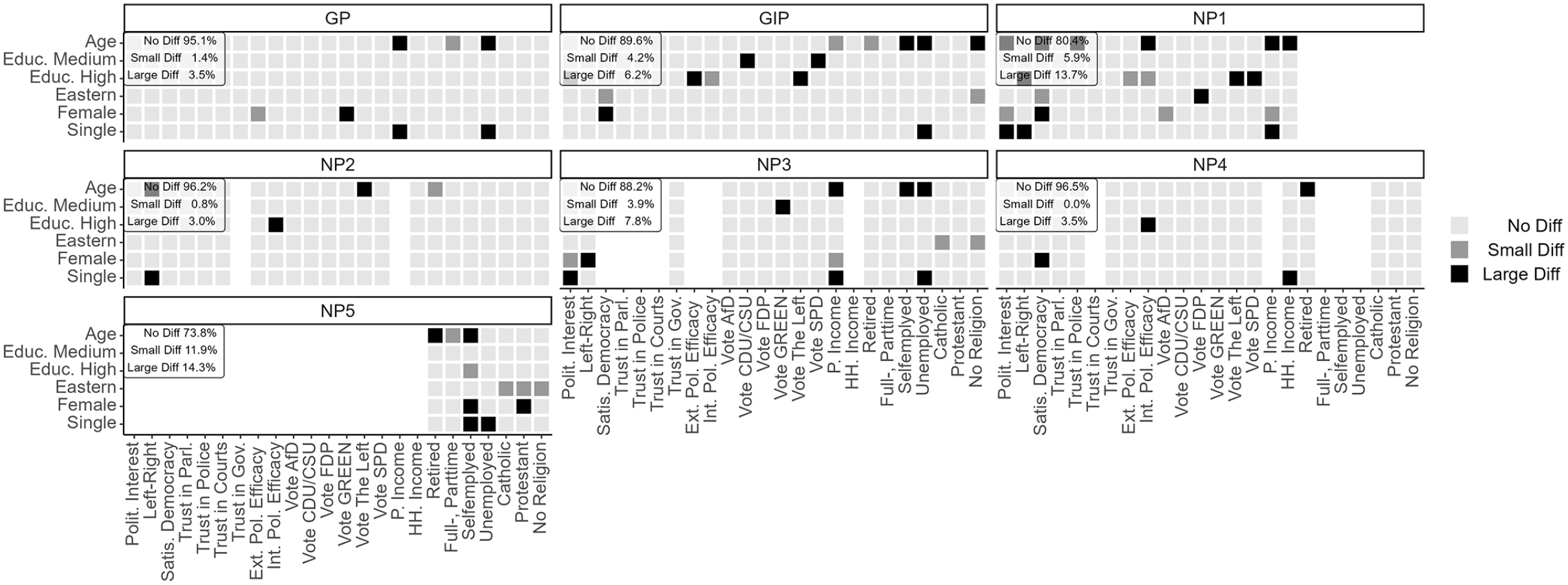
Multivariate comparison of probability and nonprobability surveys with the GGSS benchmarks: political, demographic, and religious affiliation models, Bonferroni-adjusted, weighted.
Summarizing the multivariate results regarding RQ2, the two other probability surveys (GESIS Panel and GIP) were very close to the GGSS benchmark survey. In contrast, although the nonprobability surveys were, on average, less biased than in the bivariate comparison, the similarity of the nonprobability surveys seemed to depend strongly on the individual survey, as some nonprobability surveys had a larger difference (i.e., NP1 and NP5), which indicates mixed results regarding RQ2.
Bias in Individual Variables
Addressing RQ3—whether some univariate, bivariate, or multivariate estimates are more prone to error than others in nonprobability surveys—we first investigated whether some variables were more biased on a univariate level. Most of the variables in our analyses performed very similarly regarding bias. Variables that were comparatively less accurate in one survey were more accurate in another. This was true for the demographic and the political variables. Nonetheless, for the nonprobability surveys, in two of three cases, respondents were more often retired and less often employed full-time than in the benchmark survey.
Second, in the bivariate comparison, there was more heterogeneity concerning bias across the individual variables. Although we did not see any clear pattern when comparing the demographic variables with the German microcensus, we found substantial differences when comparing the demographic and political variables with the GGSS. On the one hand, the political trust variables were prone to errors when correlated with each other. On the other hand, bias was most pronounced in the correlations between individual demographic variables, especially in surveys with a high average bias (see Figure C.1 in the online supplement).
Third, regarding the multivariate comparison, we found remarkable differences across the surveys, especially for personal income, unemployment, self-employment, and age. The models measuring personal income were the largest source of bias, accounting for 16.7 percent of all differences compared with the GGSS (13.6 percent of all differences in probability surveys, 18.8 percent of all differences in nonprobability surveys). 11 In the probability surveys, 25.0 percent—and in the nonprobability surveys, 50.0 percent—of all coefficients in the personal income models were biased. The unemployment models were also very biased (23.3 percent of all coefficients in the models). Of the secondary demographic models, the model on self-employment was also very biased in the nonprobability surveys (27.7 percent of all coefficients were different), whereas in the probability surveys, only 8.3 percent were different. We also found that some political variables (political interest, left–right, satisfaction with democracy, external political efficacy, and internal political efficacy) were more often biased in nonprobability surveys (18.6 percent of all coefficients) than in probability surveys (10.0 percent of all coefficients).
Finally, regarding the independent variables, the age coefficient differed in at least one model in every survey and was biased in 18.4 percent of all models (16.7 percent in the probability surveys, and 19.5 percent in the nonprobability surveys). Contrary to our expectation, the voting intention (4.6 percent of all coefficients) and trust variables (0.9 percent of all coefficients) had low bias in the multivariate comparisons, despite the potential time sensitivity of their measurement.
Robustness Checks
The results of the robustness checks controlling for partially varying variables across the surveys (see Part E of the online supplement) show only minor differences concerning the main results, which did not affect the substantive conclusions. More concretely, we find only minor rank changes between the surveys in each comparison, despite the different sets of variables (see Figures E.1.1 and E.1.2 in the online supplement). Similarly, the second set of robustness checks, using the same set of variables to weight each survey, shows only minor differences compared to the results using all available weighting variables (see Figures F.1 to F.5 in the online supplement). Again, this did not affect the substantive conclusions.
Comparison of Weighted and Unweighted Results
In RQ4, we investigated whether the accuracy of the nonprobability surveys increased when weighting the data. Overall, weighting was relatively successful in the univariate estimation, as it reduced the bias in some cases. When looking at the univariate demographic variables, except those that were used to construct the weights, the RMSE was reduced by up to 0.130 for NP5 (see Figure 1 and Figure D.1 in the online supplement). Weighting was also successful for the probability surveys, especially the GESIS Panel, with a bias reduction of 0.062 (RMSE). The large reduction in NP5 can perhaps be explained by the strongly biased occupation-related variables, which are likely correlated with the variables used for weighting, such as age and education. In contrast to the demographic variables, the univariate bias was less reduced for substantive variables (the RMSE was reduced by between 0.08 [NP3] and 0.025 [NP5]), and there was no noteworthy change for the GIP and the GESIS Panel (±0.001; see Figure D.2 in the online supplement).
For the bivariate comparison, weighting was overall successful in reducing bias (see Figure D.3 in the online supplement). For all surveys, weighting improved the similarity to the microcensus benchmark (e.g., by 5.4 percentage points for NP1 and by 11.7 percentage points for NP3). It was especially successful for NP5, where the similarity to the microcensus benchmark survey improved by 36.2 percentage points. For the comparisons with the GGSS benchmark survey (see Figure D.4 in the online supplement), weighting was also successful and the similarity to the benchmark survey improved for every survey (by at least 4.6 to 15.1 percentage points). NP5 again had the largest improvement (34.0 percentage points).
For the multivariate comparison (see Figure D.5 in the online supplement), weighting was overall successful in improving the similarity to the GGSS. Weighting increased the similarity to the benchmark survey for every probability survey (by 6.9 and 2.8 percentage points for the GESIS Panel and GIP, respectively) and for all nonprobability surveys (by 3.0 to 21.4 percentage points). In addition, most individual regression coefficients became more similar when weights were applied.
When comparing the weighted and unweighted results for individual variables, we found notable differences in the univariate comparison. Specifically, the weighted results for political and religious variables appear to be slightly more biased than the occupational demographic variables in the univariate comparison (see Figures 1 and 2). However, the unweighted results indicate a lower bias for political and religious variables (see Figures D.1 and D.2 in the online supplement). In contrast, when comparing results of the bivariate and multivariate estimation, we did not find notable differences between weighted and unweighted results for individual estimates (see Figures 3 to 5 compared to Figures D.3 to D.5 in the online supplement).
Discussion
In this article, we compared estimates derived from probability and nonprobability surveys to assess their accuracy on different levels. We started by comparing univariate estimates of three probability surveys and five nonprobability surveys with demographic benchmarks from the German microcensus and additional benchmarks from the GGSS. We then compared bivariate correlation coefficients for each survey with the same estimates of the benchmark surveys. Following this, we compared multivariate models estimated in the other seven surveys with the same models estimated with the GGSS. In the last step, we re-ran the analysis using unweighted data and compared the findings to the main analysis based on weighted data.
Regarding RQ1, as suggested in previous literature (e.g., Kennedy et al. 2016; Yeager et al. 2011), most nonprobability surveys showed higher bias in univariate estimates than did the probability surveys. However, some nonprobability surveys were as accurate as the GIP and the GESIS Panel. One reason the GESIS Panel was noticeably less accurate than the GGSS compared with the microcensus benchmarks might be that GESIS Panel respondents can choose between an online or offline mode. This self-selection might have introduced systematic bias, 12 as we compared only respondents who answered in the online mode. However, both probability surveys were more like the GGSS benchmarks than were most of the nonprobability surveys. Those results align with the previous literature, where nonprobability surveys are seldom as accurate as probability surveys in univariate comparisons.
Concerning RQ2, we investigated differences in bivariate relationships across the surveys. The literature is less clear on bivariate comparisons, sometimes indicating that nonprobability surveys are less accurate than probability surveys (Brüggen et al. 2016; Dutwin and Buskirk 2017; Malhotra and Krosnick 2007; Pasek and Krosnick 2020; Pekari et al. 2022) and sometimes indicating similar accuracy (Berrens et al. 2003; Dassonneville et al. 2018; Pasek 2016; Stephenson and Crête 2011). In our analyses, the results depended on the individual nonprobability survey. Whereas some nonprobability surveys differed clearly from the benchmark surveys (NP1 and NP5), others (NP2, NP3, and NP4) were similarly or slightly more accurate than the best-performing probability survey. Concerning multivariate comparisons, previous studies often compared only a few models for a small number of surveys. Those studies show mixed results, with some researchers suggesting high accuracy when using nonprobability surveys for multivariate estimation (e.g., Ansolabehere and Schaffner 2014; Dassonneville et al. 2018; Pasek 2016), whereas others found nonprobability surveys to be a disadvantage compared with probability surveys (e.g., Kennedy et al. 2016; Pasek and Krosnick 2020). In our study, the differences between probability and nonprobability surveys in multiple regression models were sometimes small. Specifically, two of the nonprobability surveys (NP2 and NP4) performed equally well as the probability surveys, but the others showed higher bias, especially NP1.
Overall, we found that one nonprobability survey (NP2) performed exceptionally well in most comparisons and, in some cases, it was even less biased than the best-performing probability survey (GGSS). Yet, one nonprobability survey (NP1) was very inaccurate in many comparisons, especially those measuring bivariate correlation estimates. This suggests that nonprobability surveys can perform well for several variables and comparisons, but the opposite can also be true. Most nonprobability surveys lay somewhere in between, and we did not find an indication of how to predict which nonprobability survey would be more or less accurate.
Surprisingly, NP4 performed better than anticipated, and sometimes even better than any other survey, although it had two relevant design limitations compared with most other nonprobability surveys. First, it included only respondents who allowed their online behavior to be tracked, and these respondents might be a selective subset of the initial respondents. Second, it did not use quota sampling, which is remarkable because quotas are supposed to improve sample composition. However, quotas improve accuracy only if the target variables are correlated to the variables used to build the quotas.
RQ3, about the role of individual variables in the overall bias, showed mixed results across the three comparisons. In the univariate comparison, we reproduced previous results, finding that occupational demographics were slightly less biased than political (see Malhotra and Krosnick 2007) and religious (see Gittelman et al. 2015) variables. For the bivariate comparison, demographic variables showed more bias than political variables, especially in NP1 and NP3. In the multivariate models, some demographic variables (i.e., personal income, unemployment, and self-employment) were more prone to bias, which is in line with Pasek and Krosnick’s (2020) findings. Additionally, we found that coefficients of some political models (i.e., satisfaction with democracy, left–right self-placement, and internal political efficacy) were more often biased in nonprobability than in probability surveys, whereas most party vote models, and especially political trust models, were less problematic.
Bias in individual variables might not only be due to misrepresentation of specific population groups but also due to errors in their measurement. Prior research has, for example, found income variables to be prone to measurement error (e.g., Einarsson et al. 2022; Gauly et al. 2019). Measurement error, in general, has been shown to differ by data collection aspects such as survey mode (e.g., Felderer, Kirchner, and Kreuter 2019) or using probability or nonprobability surveys (e.g., Cornesse and Blom 2023). Large biases for income and differences in income bias between probability and nonprobability surveys likely are due to a combination of differential selection and measurement error in both kinds of surveys.
Investigating RQ4, the results show that in line with previous findings (e.g., Brüggen et al. 2016; Dassonneville et al. 2018; Yeager et al. 2011), weighting sometimes increased the estimation accuracy and sometimes did not lead to any improvement. In univariate estimation, the improvement in accuracy was generally evident and stronger for occupational demographics than for political variables; for bivariate relationships, weighting did not result in an overall improvement. In multivariate estimation, we found improvement for most surveys, and those with a higher initial bias showed stronger improvements. As expected, the overall effect of using weights seems stronger if the variables are likely correlated with the auxiliary variables used for weighting. One should thus carefully consider whether to use weighting and, if so, which variables to select.
Beyond that, our results offer insights regarding drawing samples from the same nonprobability panel vendor. Three of our nonprobability surveys (NP1, NP2, and NP3) came from the same panel, but NP2 consistently demonstrated the lowest bias, and NP3 and NP1 showed higher bias. Notably, NP4, which came from the same vendor as NP1 to NP3 but was based on a selective web-tracking subgroup, was also relatively accurate. Consequently, using a panel vendor’s past survey accuracy does not seem adequate to predict future survey accuracy.
Our study has several limitations. First, because the benchmark surveys were conducted face-to-face and all nonprobability surveys were conducted online, we cannot be sure whether the differences resulted from the mode of data collection and were due to sampling or mode effects. To account for these mode differences, we limited the benchmark surveys and all the nonprobability surveys to Internet users (the GIP was conducted only online). Therefore, and because two of the probability surveys were also conducted online, we assume that a large amount of the observed differences across probability and nonprobability surveys were not due to mode differences.
Second, as in previous comparative studies (e.g., Brüggen et al. 2016; Pasek 2016; Pasek and Krosnick 2020), the surveys were not conducted primarily for our comparative analysis. Therefore, some design aspects, such as field periods and the use of quotas, differed. However, except for political variables, the examined variables were not expected to be time-sensitive, and we could assess their time-sensitivity. Also, one of the least accurate surveys (NP1) and one of the most accurate surveys (NP2) were both conducted in the same year as the microcensus (main benchmark survey), so the date of data collection could not explain the differences in accuracy.
Third, we did not identify the source of the observed bias in the individual variables. Future studies could build on our findings by implementing theory-driven analyses on why some variables might be less robust in nonprobability surveys. Fourth, we did not receive weights from the survey providers, which would have allowed us to compare our own with the provided weights. Yet, previous research (e.g., Chang and Krosnick 2009; Craig et al. 2013) indicates that provided weights do not adequately correct the biases of nonprobability samples. The fifth limitation of our study is that it included only surveys from Germany. Looking forward, it would be interesting to compare bivariate and multivariate estimates in a cross-national context. Non-Western countries, in particular, have been largely unexplored concerning sample comparisons (as a recent exception, see Castorena et al. 2023).
In conclusion, we can state that if used for a purpose that aligns with their generalizability limitations (Jerit and Barabas 2023), nonprobability surveys can be a viable instrument in the social scientist’s toolkit. Although we found it problematic to use nonprobability surveys in univariate estimation, bivariate and multivariate estimation led to comparably more accurate results. Still, the usefulness of nonprobability surveys for one’s respective research question should be carefully considered, as in some multivariate models—such as those including income, unemployment, left–right self-placement, and age—coefficients were substantially biased.
Supplemental Material
sj-pdf-1-smx-10.1177_00811750241280963 – Supplemental material for Comparing the Accuracy of Univariate, Bivariate, and Multivariate Estimates across Probability and Nonprobability Surveys with Population Benchmarks
Supplemental material, sj-pdf-1-smx-10.1177_00811750241280963 for Comparing the Accuracy of Univariate, Bivariate, and Multivariate Estimates across Probability and Nonprobability Surveys with Population Benchmarks by Björn Rohr, Henning Silber and Barbara Felderer in Sociological Methodology
Footnotes
Supplemental Material
Supplemental material for this article is available online.
Notes
Author Biographies
References
Supplementary Material
Please find the following supplemental material available below.
For Open Access articles published under a Creative Commons License, all supplemental material carries the same license as the article it is associated with.
For non-Open Access articles published, all supplemental material carries a non-exclusive license, and permission requests for re-use of supplemental material or any part of supplemental material shall be sent directly to the copyright owner as specified in the copyright notice associated with the article.