
Abstract
In this article, we explore the use of Facebook targeted advertisements for the collection of survey data. We illustrate the potential of survey sampling and recruitment on Facebook through the example of building a large employee–employer linked data set as part of The Shift Project. We describe the workflow process of targeting, creating, and purchasing survey recruitment advertisements on Facebook. We address concerns about sample selectivity and apply poststratification weighting techniques to adjust for differences between our sample and that of “gold standard” data sources. We then compare univariate and multivariate relationships in the Shift data against the Current Population Survey and the National Longitudinal Survey of Youth 1997. Finally, we provide an example of the utility of the firm-level nature of the data by showing how firm-level gender composition is related to wages. We conclude by discussing some important remaining limitations of the Facebook approach, as well as highlighting some unique strengths of the Facebook targeted advertisement approach, including the ability for rapid data collection in response to research opportunities, rich and flexible sample targeting capabilities, and low cost, and we suggest broader applications of this technique.
The virtues of probability sampling—in which samples are selected at random and sample members have a known probability of selection—are many and well appreciated. Foremost among these benefits is the ability to generalize from samples and draw valid inferences about populations. Importantly, realizing this benefit requires a sampling frame that accurately captures the target population and nondifferential response to the survey invitation. For some hidden and hard-to-reach populations, sampling frames do not exist and probability sampling has never been an option, creating some impetus for developing tools for drawing inferences from nonprobability sampling methods.
Further, increasingly, even for populations for which probability sampling has historically predominated, serious obstacles have arisen that add urgency to the task of finding alternative sampling and data collection techniques. For instance, the decline in the coverage of landlines has undermined the primary sampling frame for telephone surveys, and telemarketer fatigue and technology that facilitates call screening and call blocking have dramatically reduced survey response rates. As a result, response rates to nongovernmental surveys have plummeted. For instance, at one of the nation’s leading polling organizations, Pew Research, the response rate has dropped from 36 percent in 1997 to 9 percent in 2016 (Keeter et al. 2017). The natural concern is that the 1 in 10 individuals who do still respond to surveys could be substantially different from those who do not—that is, that probability samples cannot be seriously considered random samples of the population or at the least that total survey error is increasingly high.
In response to this urgent need for new data collection strategies, there have been important advancements in developing methods of nonprobability sampling for addressing bias and yielding valid inferences (Zagheni and Weber 2015). Recent research has shown that, using poststratification weighting techniques to weight to gold standard sources such as the census on demographics, even surveys with very low response rates exhibit little evidence of bias on univariate statistics or bivariate relationships (Kohut et al. 2012), with the main exception being measures of civic engagement (Keeter et al. 2017). This insight has led a new generation of survey researchers and statisticians to suggest that it is then worth revisiting the value of nonprobability sample surveys (Goel, Obeng, and Rothschild 2015; Wang et al. 2015).
Over the past several years, scholars have begun to take up this call and have creatively harnessed data from such sources as Twitter, e-mail, and Google searches to study migration, fertility, and other demographic processes (Billari, D’Amuri, and Marcucci 2013; Reis and Brownstein 2010; Zagheni and Weber 2012; Zagheni et al. 2014). Researchers have also conducted online surveys using a range of online nonprobability samples (Couper 2017). These approaches appeal in part because they can be quickly implemented at generally very low cost (Goel et al. 2015; Nunan and Knox 2011; Stern, Bilgen, and Dillman 2014).
But the research community has been divided on the scientific value of research using surveys collected from online nonprobability samples. The weight of early research and discussion suggested that problems of undercoverage from limited and selective Internet usage made this approach of limited use (Best, Krueger, and Hubbard 2001; Bethlehem 2010; Yeager et al. 2011). Research continues to point to problems both with point estimates and relationships between variables in nonprobability online opt-in panel surveys (Bruggen, Brakel, and Krosnick 2016; Casler, Bickel and Hackett 2013; Dutwin and Buskirk 2017).
However, recent research has found more encouraging results for online nonprobability samples recruited through websites and advertising such as through Mechanical Turk, the X-Box gaming console, and Google ad words. This work suggests that such Internet-based samples can fairly closely resemble probability samples in terms of demographics (Stern et al. 2014) and, further, perform well when weighted, in terms of yielding results in line with benchmark samples that use more conventional probability sampling approaches (Clifford, Jewell and Waggoner 2015; Goel et al. 2015; Wang et al. 2015; Mullinix et al. 2015).
Yet, of all nonprobability web-based recruitment platforms employed to date, Facebook has the largest user base, has broad global coverage, exhibits less selection than for opt-in panels, and validates respondents’ identities. Some prior work has used snowball sampling on Facebook through affinity groups to collect surveys (Baltar and Brunet 2012; Bhutta 2012) and this work generally finds that associations from the resulting data resemble those estimated from standard data sets such as the General Social Survey (Bhutta 2012). Other recent work in marketing (Nunan and Knox 2011), medical research (Ramo and Prochaska 2012; Thornton et al. 2016), and political science (Samuels and Zucco 2013; Zhang et al. 2017) has begun to explore the use of Facebook advertisements to recruit respondents to surveys. These studies have generally attempted to use Facebook to develop samples meant to approximate the general population. Recently, demographers have demonstrated that the Facebook advertising platform can be used as a “digital census” and employed it to estimate migrant populations by country and U.S. state (Zagheni, Weber, and Gummadi 2017).
Building on insights from this recent research, we suggest that a unique benefit of sample construction on Facebook is the ability to use the detailed audience targeting capabilities that are at the heart of Facebook’s advertising model to construct samples of otherwise difficult-to-sample populations (a point also alluded to in American Association for Public Opinion Research [AAPOR] 2014; Zagheni, Weber, and Gummadi 2017). We suggest that one such population of particular academic and policy interest is the employees of specific named firms. Such employer–employee linked data would be valuable to economic sociologists, who are interested in understanding how firm-level characteristics such as ownership structure and unionization affect labor practices (Applebaum and Batt 2014; Fligstein 2001; Weil 2009); to policy scholars, who are interested in assessing the impact of local and state labor laws that focus on specific large employers (Colla et al. 2014); and to economists who are concerned with measuring intraindustry variation in compensation (Andersson, Holzer and Lane 2005; Groshen, 1991a, 1991b; Krueger and Summers 1988; Lane, Salmon and Spletzer 2007).
However, this sort of employer–employee matched data has proven elusive to social scientists. Data sets that are commonly used to describe employees’ job conditions such as the NLSY, Panel Survey of Income Dynamics (PSID), or Current Population Survey (CPS) do not allow a link to identifiable employers. Studies, such as the National Organizations Survey, that contain detailed data on firm practices do not contain data from multiple employees at a given firm. Restricted access employer–employee linked data such as the Longitudinal Employer-Household Dynamics (LEHD) or the Bureau of Labor Statistics’ Occupation Employment Statistics (OES) are limited by not publicly identifying employers and by having a fairly circumscribed set of measures. An important constraint on this work has been the absence of a sampling frame of workers at a large set of specific companies and the significant cost of attempting to assemble such a sample from a general population survey.
We illustrate the potential of survey sampling and recruitment on Facebook through the example of building just this sort of employee–employer linked data set for The Shift Project. We discuss the workflow of using the Facebook advertising platform, describe the results of our data collection efforts, discuss useful strategies for poststratification and weighting, and then compare key associations from our data with a range of survey data gathered using probability sampling methods. We then take up the important question of selection into the survey on unobservable attributes that cannot be easily accounted for with weights and propose an easily implemented test to gauge the significance of this problem. Finally, we exploit the firm-level structure of the data to estimate how firm-level gender composition is associated with wages. Our results show that this data collection approach yields data that are broadly consistent with gold standard probability samples at the national level and open up rich opportunities for granular targeting of a variety of hard-to-reach populations. However, we also note some of the important limitations of this approach.
Targeted Advertising on Facebook
Using Facebook to collect survey data departs from traditional probability sampling and some have raised reasonable questions about such approaches (Groves 2011; Smith 2013). One potential concern arises from the sampling frame of Facebook users. In the recent past, both Internet access and Facebook use have been confined to relatively narrow subgroups of the population, which tended to have relatively high socioeconomic status. However, Internet access is now widespread in the United States among working-aged adults. Recent estimates from the American Community Survey find that between 90 percent and 94 percent of working-aged adults have a computer at home and between 80 percent and 84 percent have broadband Internet access at home (Ryan and Lewis 2017). Among those who use the Internet, the very large majority are active on Facebook—79 percent overall and 86 percent of those 18–49 (Greenwood, Perrin and Duggan 2016). The result is that 81 percent of Americans aged 18–49 are now active on Facebook, far in excess of the percent of this population with landlines. Further, although people of color and low-income strata are less likely to have home computers and broadband access (Ryan and Lewis 2017), Facebook use is nevertheless not especially stratified by demographic characteristics (Greenwood et al. 2016). In addition, unlike some online platforms, Facebook goes to some length to verify that each user account is associated with a unique identifiable person (Facebook 2017).
Facebook has two other important advantages over both phone and address-based sampling. First, unlike phone and address-based sampling, the Facebook profile is a portable and durable means of contact. Respondents can be reached by Facebook for survey recruitment whether at home or work, whether they have moved or have a long residential tenure, and whether they change phone numbers or lose service. This represents a distinct advantage over conventional sampling frames.
Second, Facebook collects detailed data on the attributes of users that can be used by advertisers to target their campaigns quite precisely. Indeed, this capability is at the heart of Facebook’s business model. These attributes include standard demographics such as age and gender, locational attributes, interests, and information on schooling and employment. This last field permits us to deliver advertisements that are targeted to users who work at specific firms. Given the goal of assembling a data set that includes large samples of workers at each of a large number of firms, this targeting capability is very valuable.
To illustrate, consider the effort that would be associated with assembling a sample of this type using traditional methods. Given that a large number of employers are unlikely to be persuaded to turn over lists of employees with contact information, one would need to begin with a nationally representative sampling frame (such as a purchased phone or address list) that would not contain any information on employer, screen on those in the labor force, then those currently employed, then those in the sector of interest, and then those at particular large companies. To take just one example, Walmart is far and away the largest private sector employer in the country with 1.4 million employees. However, that equates to just 0.055 percent of the 255,000,000 U.S. adults. Given response rates of approximately 9 percent for nongovernmental surveys (Keeter et al. 2017), that would entail attempting to contact approximately 404,00 adults by phone or mail to achieve a sample of 200 Walmart workers ((200/.09)/.0055). Given a survey, such as ours, that aimed to collect data from 200 workers at each of 40 large companies with collective employment of 6.9 million, one would need to contact approximately 3.3 million adults.
Data Collection
Acting as an “advertiser,” we use Facebook’s audience targeting tools to purchase and place survey recruitment advertisements in the newsfeeds of Facebook users who work at specific companies. Each advertisement was targeted to employees of a specific company (or family of consumer-facing brands), in the 18–50 age range, who were located in the United States. The availability of targeting by employer name was a key feature that made this data collection approach viable for our research purposes. Notably, the feasibility of using Facebook targeted advertisements for survey recruitment crucially depends upon Facebook offering targeting options that fit the research topic at hand.
Facebook provides several options for the “marketing objective” of the campaign. Our default approach, selected after consultation with advertising specialists at Facebook, is to set the campaign objective as “traffic,” which equates with the goal of having Facebook users click the link embedded in the advertisement that takes them to our online survey. Facebook also provides the option to set a campaign objective that equates with increasing “awareness” or of increasing “conversion.” How the Facebook advertisement algorithm actually translates these different objectives to differential ad placement is something of a black box and the inability for researchers to fully map the display process is a significant limitation of this approach. Additionally, as a private corporation, Facebook has the power to change the display algorithm with little notice or clear explanation. If such changes lead to differential selection into the sample on unobservables, then samples collected over time may be differentially biased in unknown ways.
Advertisements appearing on Facebook must follow a fairly standardized design, but there are options within that framework. For instance, while every advertisement must link to a Facebook page, include a headline and advertisement text, an image, and may include a link to an external webpage, advertisers have substantial discretion in crafting the advertising text, in choosing the content of the image, and in using a single image as opposed to a carousel, a video, a slideshow, or a collection.
We used a simple template for all of our advertisements. Every advertisement included a single image drawn from licensed stock photography available at no charge on the Facebook advertising page. We selected images that seemed to most closely approximate an employee of the target company at work, matching on store environment and color and style of employees’ uniforms. Every advertisement linked to a UC Berkeley Work and Family Study” Facebook page that itself included very little additional content. For the data reported on in our main analysis, every advertisement used the “headline” field to offer users the opportunity to enter a drawing for an Apple iPad. Finally, again for the data in our main analysis, every advertisement used the advertisement text field to include a standard recruitment message. This message took the form of “Working at <targeted employer>? Take a short survey and tell us about your job!” In Figure 1, we include sample advertisements that we have used to recruit workers to the survey.

Examples of employer-specific survey recruitment advertisements placed on Facebook.
Finally, Facebook offers various options for advertisement placement. Advertisers may opt to have their advertisements appear on Facebook (in the newsfeed and/or in the right-hand column on desktop), on Instagram, or on partner networks. All of our campaigns were placed on Facebook in the newsfeed and on Instagram. Users who click on the advertisement are routed to an electronic survey hosted by Qualtrics-XM. The survey can be accessed on desktop or mobile devices. Users are asked to consent to participation and then begin the survey. In essence, Facebook serves as both the sampling frame and the recruitment channel.
Survey Data
Our survey includes five core modules. The first collects information on respondents’ jobs including on job tenure, hourly wage, hours, benefits, and work scheduling practices. The second module collects information on respondent’s household economic security including household income, public benefits use, and use of alternative financial services. The third module contains data on respondents’ demographics. The fourth module assessed respondents’ health and well-being including self-rated health, sleep quality, and depressive symptoms. The final module was asked of parents and included information on child well-being, parenting time, and childcare. The individual survey questions were drawn from existing large-scale surveys including the Fragile Families and Child Wellbeing Survey, the National Longitudinal Survey of Youth 1997 (NLSY97), and the National Health Interview Survey (NHIS).
We fielded recruitment advertisements to Facebook users employed at 38 large retail firms, drawn from among the 100 largest retail firms by revenue in 2015 (National Retail Federation 2015). We fielded these advertisements between September 2016 and June 2017. In total, our advertisements were shown to 3,270,228 Facebook users, including some who were shown one of our advertisements on more than one occasion. These advertisements generated 179,563 link clicks through to the introductory page of our survey at a total advertising and prize cost of $75,000. Then, 39,918 respondents contributed at least some survey data. In all, 5.3 percent of our advertisement views led to a click-through to begin the survey and 22 percent of those individuals contributed some survey data (or 1.2 percent of all advertisement views), for an average cost of $1.88 per respondent.
Of the 39,918 respondents who contribute some survey data, we eliminate 6,468 respondents who report that they were not paid hourly. In addition, the survey included a data quality check that instructed respondents to select a specific option on a question. Ninety-six percent of respondents who were presented with this item complied. However, this item was not asked of respondents who attrited early in the survey. The result is a sample of 32,142 respondents.
However, there was substantial attrition. Of the 32,142 respondents who began, 17,828 fully completed the survey, and among those, there was item nonresponse. We perform multiple imputation to account for this missing data. First, we impute data only for those respondents who completed the survey but had item nonresponse. Second, we impute data for all respondents who completed the first survey module, including those who finished the survey with some item nonresponse and those respondents who attrited from the survey at various points.
Our final analysis sample for a single implicate using the first approach is 17,828 responses and for the second imputation approach is 29,722 responses, both distributed across 38 companies. Based on the first sample size, the average price per survey response was $4.21 and based on the second it was $2.52. With complete or imputed data for each respondent on 125 items, we estimate a per item cost of $0.034 and $0.02. If we only consider complete items, we estimate a per item cost of $0.036 and $0.028 for the two samples. These estimates are very similar to the cost that Goel, Obeng, and Rothschild (2015) report for their survey using Amazon Turk—and at least 20 times cheaper than traditional Random Digit Dial polling (Goel et al. 2015) on a per question basis and far more inexpensive even than that given the focus on employees of these 38 companies. However, an important caveat is that these cost estimates only include advertising and incentive costs, not staff time for survey programming, advertisement placement, or data processing. Moreover, the costs reported here are specific to an advertising/recruitment campaign focused on users employed at specific firms. While we expect that these costs would be similar for other targeted audiences (Ad Espresso 2018), it is possible that precise costs would vary based on the salience of the group identity, the sociodemographics of the targeted population, and the size of the targeted audience.
All of the analyses we describe below produced substantially similar estimates when using the imputations on the sample of 29,722 responses versus 17,828 responses. For the sake of parsimony, we present only the analysis on those who completed the survey, with multiple imputation for item nonresponse (n = 17,828).
Poststratification and Weighting
A concern with using a nonprobability-based sample, such as this one, is that respondents may differ from the target population. Sample overrepresentation on particular demographic attributes can be addressed using poststratification and weighting of the survey data to a “gold standard” benchmark (Zagheni and Weber 2015).
A key contribution of our application is to construct a survey sample that contains relatively large numbers of employees at each of several dozen employers. This is valuable precisely because such data are not readily available from existing survey or administrative sources. The consequence is that it is actually somewhat difficult to derive a good estimate of the demographic characteristics of our target population to use as a benchmark. Our solution is to compare the demographics of our survey respondents against several candidate benchmark populations, none of which exactly capture our target population. This same problem, that the rationale for using a Facebook approach stems at least in part from the lack of suitable existing data and thus a lack of data that can be used to construct weights, is likely to arise for other applications as well.
First, we pool data from the 2013 to 2015 American Community Surveys (ACS). We condition the ACS sample on respondents being age 18–55 and employed in industries in the retail sector (581, 591, 600, 601, 623, 633, 641, 642, and 691) that are represented by the 38 companies. We exclude any of these respondents who report upper-level managerial occupations. In total, we have data on 482,608 ACS respondents who meet these inclusion criteria.
Second, we pool data from the 2010 to 2017 rounds of the CPS, focusing on the March Annual Social and Economic Supplement (ASEC). The ASEC is valuable because while the sample size is smaller than the ACS, the ASEC includes a measure of firm size that captures whether the respondent works at a firm with greater than 1,000 employers. While all of the firms in our data have substantially more than 1,000 employees, conditioning on this variable at least allows us to exclude the many retail workers who are employed at small nonchain firms from our analysis. Here too, we further condition the sample to those aged 18–55 who work in the relevant industries and occupations. In total, we have data on 32,221 CPS-ASEC respondents who meet these inclusion criteria.
Third, we extract data from the Facebook advertising platform on the demographics of users who work at each of the companies in our data. While the survey data provide us with the demographics of those who took the survey, we can get demographic information on the characteristics of all potential respondents from the Facebook sampling frame by drawing on the advertising platform. Further, while in ACS, we can only generate a benchmark population of those in the comparable industry and in the CPS-ASEC only of those in the comparable industry and at large firms, with the Facebook data, we can benchmark to the demographics of those at the very same company. The trade-off is that we benchmark to those who are on Facebook rather than to the broader population of all workers employed at those companies. Additionally, the demographic information available from the Facebook advertising platform is limited to respondents’ age and gender.
We categorize our benchmark samples in terms of the matrix of demographic characteristics. We also create a variant that further stratifies by industry. For our ACS and CPS-ASEC benchmark samples, we stratify respondents into cells defined by Age × Race/Ethnicity × Gender × Industry Group. For these benchmarks, we categorize age into three bins (18–29, 30–39, or 40–55), race/ethnicity into four mutually exclusive bins (white, non-Hispanic; Black, non-Hispanic, Other or two or more races, non-Hispanic, or Hispanic), gender into two categories (male or female), and industry into nine groups (hardware, department stores, general merchandise, grocery, fast food, apparel, electronics, drug store, or other retail). For our Facebook benchmark, we construct a Matrix of Age × Gender × 38 Employer Cells.
We then construct weights for each cell that are the ratio of the proportion of the benchmark sample in each cell to the proportion of our sample in that same cell. The intuition behind these weights is that when a particular subgroup is relatively larger as a proportion of the benchmark sample than it is in our sample, then this group will be upweighted with a weight value that is greater than 1. Conversely, when a subgroup is relatively smaller as a proportion of the benchmark sample than it is in our sample, then this group will be downweighted with a weight value less than 1.
Finally, we further account for variation in the number of employees who work at each of the firms in our data by adjusting the individual responses by company labor force size to correct for any over or underrepresentation of employees at particular companies in our survey data relative to the actual relative labor force of a given company (e.g., the share of respondents in our survey data who work at Walmart might either be too large or too small a percent of all respondents as compared to Walmart’s share of total employment at the 38 companies in our data). To make this correction, we use detailed data on establishment-level employment from the ReferenceUSA U.S. Businesses database, collapsing thousands of store-level records to generate total in-store employment at each of the 38 companies.
The result is a set of eight weights: (1) ACS by demographics, (2) ACS by demographics/industry, (3) ACS by demographics/industry with employer size correction, (4) CPS by demographics, (5) CPS by demographics/industry, (6) CPS by demographics/industry with employer size correction, (7) Facebook by demographics/employer, and (8) Facebook by demographics/employer with employer size correction.
Table 1 compares the unweighted demographics of our survey respondents (column 1) against each of these benchmarks—the ACS (column 2), the CPS-ASEC (column 3), and Facebook users (column 4). The table shows that the unweighted Shift sample is disproportionately female, young, and white, non-Hispanic compared with the broader population in the ACS and CPS samples. While we do not have information on race/ethnicity for Facebook users, for gender and age, our sample is more similar to the Facebook user population employed at these firms, though by no means identical.
Comparison of Key Demographics in Shift, ACS, CPS-ASEC, and Facebook.
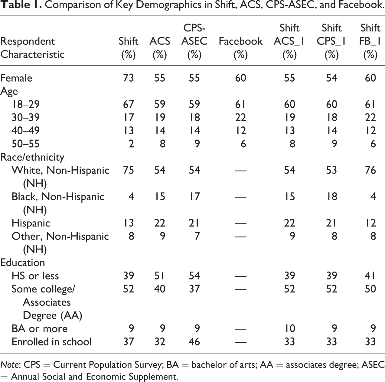
Note: CPS = Current Population Survey; BA = bachelor of arts; AA = associates degree; ASEC = Annual Social and Economic Supplement.
The next set of columns tabulate the Shift data by gender, age, and race/ethnicity after applying the basic weights to the ACS, the CPS-ASEC, and Facebook. We see that the weighting procedure clearly brings the Shift sample into alignment with these benchmarks in terms of gender, age, and race/ethnicity.
We also compare educational attainment and school enrollment in the unweighted Shift data against the ACS and CPS and then against the weighted Shift data. Here, we again see some discrepancies in educational attainment. However, most of the difference appears to be from those who have completed “some college” which is difficult to accurately assess. The share that reports a college degree is constant across the unweighted Shift, the ACS, the CPS, and the weighted Shift estimates. We also see that the estimate of school enrollment—37 percent—in the unweighted Shift data is between the somewhat lower estimate in ACS (32 percent) and the higher estimate in CPS (46 percent).
Comparison With National Surveys
As previously mentioned, an important rationale for developing this method of survey recruitment using Facebook is to address a lack of available data. Although the employer–employee linked database that we have compiled is unique, we can make some comparisons of tabulations from our data set to overlapping measures available in two widely used and carefully constructed probability sample national surveys: the NLSY97 and the CPS. In particular, we estimate and compare (a) regression-adjusted wages, (b) job tenure, and (c) the relationship between job tenure and wages from the Shift data and from the NLSY97 and CPS data sources.
Both the NLSY and CPS surveys aim to assemble a representative sample of the U.S. population—the NLSY97 for the cohort born between 1980 and 1984 and the CPS for the noninstitutionalized population over the age of 15. In contrast, the Shift survey aims to recruit respondents in a target population of retail workers under the age of 55 who are paid hourly and work at large firms. Additionally, the CPS has been fielded from 1962 to 2016 and the NLSY97 from 1997 to 2013, while the Shift data were collected in 2016 and 2017. Our first step then is to align the three samples as closely as possible. We select cases from the most recent rounds of the NLSY97 (2011 and 2013) and from the CPS (2010–2016). We next restrict both samples to respondents who are paid hourly and who work in the industries represented in our data (581, 591, 600, 601, 641, 623, 633, 642, and 691 in the Industry 1990 codes). The 2011 and 2013 rounds of the NLSY97 only include respondents between the ages of 26 and 34. But, the CPS includes respondents of a wide range of ages, and we restrict to those aged 18–55 to align with the Shift data.
We then construct harmonized measures across the CPS, NLSY97, and Shift samples of several core variables: hourly wage (inflation adjusted using the Consumer Price Index [CPI]), job tenure, gender, age, and survey year. In total, we have 17,828 observations in the Shift data, 1,518 observations in the pooled CPS, and 1,494 observations in the pooled NLSY97. We apply the survey weights from the CPS or NLSY97 and we estimate the models on the Shift data using each of our constructed weights.
While the measures are harmonized, the samples from the CPS, NLSY97, and Shift are still not exactly comparable. First, the survey years differ—the NLSY97 data are available for 2011 and 2013; the CPS for 2010, 2012, 2014, and 2016 (when the job tenure module was asked); and the Shift data for 2016 and 2017. Second, the age range in the NLSY97 is much narrower than in the CPS and Shift. Third, the Shift data come from employees of large firms, while the CPS and NLSY data are for the entire sector, regardless of firm size.
To make comparisons between these three data sets, we first estimate mean values of two key employment characteristics—hourly wage and tenure—after adjusting for age, gender, and indicator terms for year of survey. We compare the estimates from the Shift, CPS, and NLSY97 data. Table 2 shows the regression-adjusted mean wages and distribution of tenure by survey. We estimate wages with an Ordinary Least Squares (OLS) model as a function of tenure, age, gender, and year, and we estimate tenure with a multinomial logistic regression model as a function of wages, age, gender, and year. We estimate these models separately for each combination of Survey × Weight. Mean hourly wages are similar across the three surveys—$10.31 in the CPS, $12.58 in NLSY97, and between $10.95 and $11.74 in the Shift data, depending on the weight.
Comparison of Mean Hourly Wage and Job Tenure in Shift, CPS, and NLSY97.
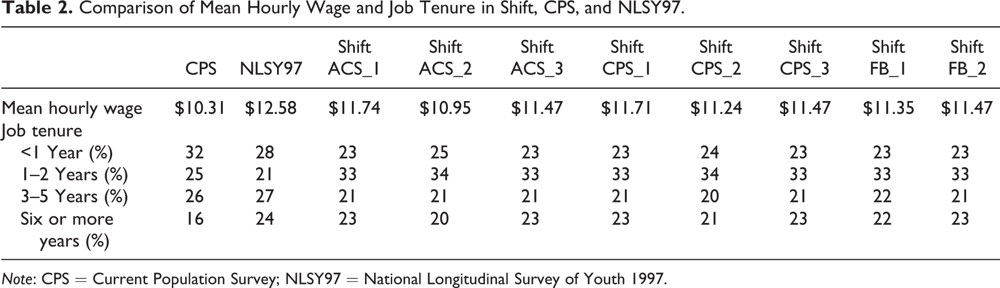
Note: CPS = Current Population Survey; NLSY97 = National Longitudinal Survey of Youth 1997.
The magnitude of the difference in adjusted mean wages between the Shift data (using each of the eight poststratification weights) and the CPS data ranges from 64 cents to $1.42. These differences in adjusted mean wages between the Shift and CPS data sources equate to in the range of 1/10 to 1/4 of a standard deviation difference (this range applies to the standard deviation of wages from either data source). Whether this amount of discrepancy between data sources is considered small, moderate, or large is a matter of judgment and depends on the precision needed to pursue particular research objectives. We would characterize these differences as “not large.”
The magnitude of the difference between the adjusted mean wages between the Shift data and the NLS data is similar, ranging from an 84 cent to a $1.63 difference, or about a 1/10 to 1/4 of a standard deviation.
When we test the significance of the differences between these adjusted means, assuming that the data from the CPS, NLSY, and Shift surveys represent independent samples, we find that the differences in means between all data sources are statistically significant. However, an important caveat and reminder when assessing the significant differences across data sources is that the CPS and NLS represent imperfect “ground truth” estimates for the Shift data because of inherent differences in sample composition between these data sources. For instance, some of the discrepancy between these sources may stem from true differences between these samples that are not related to bias or error, for instance, because the CPS and NLS include employees working for small firms and the Shift data do not.
There are more substantial differences between the surveys in the distribution of tenure. Here, close to a third of CPS respondents have less than one year of tenure as compared with 28 percent of those in NLSY and about a quarter of shift respondents. In contrast, a higher share of Shift respondents is estimated to have one to two years of tenure than the share of CPS or NLSY97 respondents. In turn, smaller shares of Shift respondents report three to five years of tenure as compared with CPS and NLSY97. The share with six or more years of tenure is similar in NLSY97 as in Shift, but lower in CPS. In no case do the numbers precisely agree across all three sources, but in no case are they substantially different, either.
Next, we examine whether the well-documented relationship between job tenure and wages varies across the three surveys. For each of the surveys, separately (and separately for each of the eight Shift weights), we regress wages on tenure, controlling for age, year, and gender.
Figure 2 presents the key coefficients from these models. Compared with having less than a year of tenure, we see in the left panel that those with one to two years of tenure receive a wage premium. The estimated size of this premium is fairly stable across the eight estimates using the eight weights from the Shift data—about $0.60. We see that this estimate also falls between the low estimate of essentially no return to one to two years of tenure in the CPS data and the estimate of about $1.30 in the NLSY-79 data. In the middle panel, we present the estimates of the return to wages of having three to five years of job tenure. Again, the estimated premium about $1.80 is stable across the Shift estimates and is somewhat higher than in the CPS and somewhat lower than in the NLSY97. In both cases, the Shift estimates are closer to both the NLSY and the CPS estimates than these two data sources are to each other. The right-hand side panel presents the estimates of the returns to six or more years of tenure. Here, we see more variation in the estimated returns across the eight Shift estimates, ranging between $4.00 and $5.00, but again, essentially falling between the NLSY97 and the CPS estimates. In Figure 3, we plot out the predicted wage values by tenure for each of the eight Shift estimates and then for the NLSY97 and CPS. As we would expect given the coefficients, we see approximately parallel lines with a higher intercept for the NLSY97 and a lower intercept for the CPS.
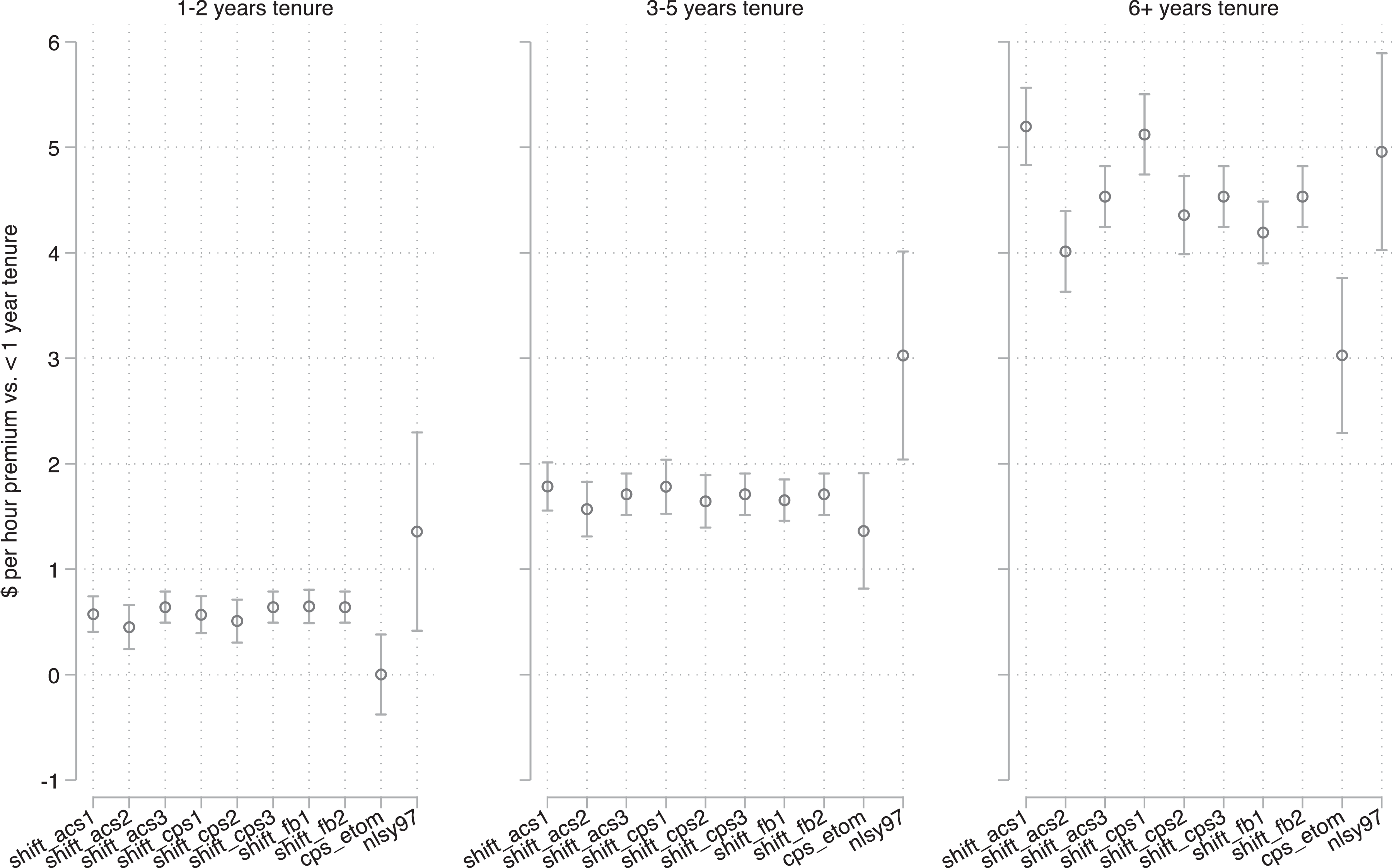
Association between job tenure and inflation adjusted hourly wage in the Current Population Survey (2010–2016), National Longitudinal Survey of Youth 1997 (2011–2013), and Shift (2016–2017) surveys. Adjusted for age, gender, and survey year.
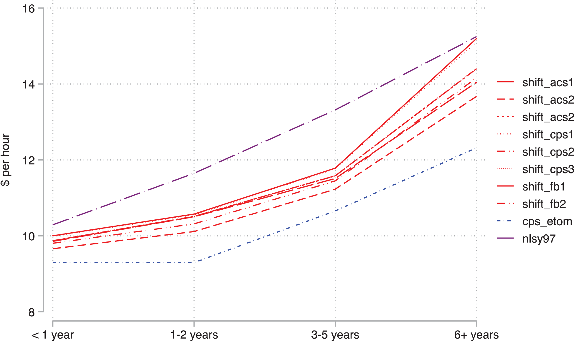
Predicted wages by job tenure in the Current Population Survey (2010–2016), National Longitudinal Survey of Youth 1997 (2011–2013), and Shift (2016–2017) surveys. Adjusted for age, gender, and survey year.
The graphical evidence that the Shift data estimates of the tenure/wage relationship are closer to the NLS and CPS than these sources are to one another is reassuring. However, in other applications, researchers may not have multiple gold standard benchmarks or the estimates from a nonprobability Facebook-drawn sample may not be bounded by gold standard benchmarks. Therefore, a more universal means to assess the differences between coefficient estimates across sources is to simply assess the statistical significance of differences in coefficient estimates between data sources. We do so by differencing the coefficient estimates between the Shift and either NLS or CPS data sources, then dividing by their pooled standard errors to generate a z statistic (Clogg, Petkova and Haritou 1995). For the Shift versus NLS comparisons, we find that coefficient estimates of the wage returns to one to two years or six or more years of tenure are not statistically different, but the differences in estimates of the returns to three to five years of tenure are statistically significant (a $3 wage return to three to five years on the job in NLS compared with $1.80 in the Shift data). When comparing Shift and CPS data, we find that the wage returns to one to two years or six or more years of tenure are significantly different and are greater in the Shift data compared with CPS, but the wage returns to three to five years of tenure are not significantly different. Again, we must keep in mind that the differences in estimates between data sources could come about because of bias or error in the nonprobability Shift data but also because of differences in sample composition across the data sources that we could not fully account for in our analysis.
In sum, these comparisons of univariate statistics and multivariate relationships between Shift and two high-quality probability sample surveys are encouraging. On wages and tenure, Shift is no more different from the NLSY and the CPS than they are from each other. It is important to note that Shift is not identical to either of the other surveys. But, by comparing against two probability sample surveys, we see that no two of the surveys are identical to each other.
Test of Selection on Unobservables
We poststratify and weight our survey data to account for bias on observable demographic characteristics. And, we find that the weighted data can closely replicate established associations from the CPS and NLSY97. However, it remains possible that our estimates could be biased by selection into the Shift survey on unobservables.
Here, we describe a test of the presence of such selection on unobservables that leverages the particular dynamics of advertising on Facebook and that would be available to anyone who used paid advertising to field a survey. We recruited respondents to the survey through paid advertisements on Facebook. We specified our target audiences and our advertisements were delivered to eligible users based on Facebook’s advertisement placement algorithm. However, a unique feature of Facebook’s paid advertisements is that users can engage with these paid posts in much the same way that they may engage with posts created by friends or institutions.
Facebook users can share the advertisement to their own time lines or those of their friends. The extent of this sharing can be gauged by the “social reach” of an advertisement in terms of the number of unique users who see the advertisement through social channels and in terms of the number of “social impressions” obtained through such channels. These may then generate “social clicks” in which users click through to the survey from a social share rather than from a paid placement.
Respondents who take our survey because their friends shared the content are likely to be different in meaningful ways than those who are targeted by our paid advertisements. Further, this social sharing may extend the reach of our advertisements beyond those who list their employer to those who do not list an employer, but whose employer is known to friends on Facebook. We leverage the fact that these forms of social engagement with our advertisements are then likely to shift the pool of respondents to the survey and introduce heterogeneity in the composition of the sample at the level of the recruitment advertisement. However, we are not able to use this information to identify a particular source of unobserved heterogeneity or even its extent. Rather, we suggest that this social sharing process is likely to introduce some heterogeneity on unobservables and can thus test if this unspecified unobserved heterogeneity is an important source of bias. To do so, we compare those who came to the survey through advertisements that experienced high levels of social sharing with those who came through advertisements with little such social activity. Although the expected direction of potential bias is uncertain a priori, if unobserved characteristics bias our estimates, we should see a significant interaction between the extent of social sharing and job tenure on wage rates. We cannot, however, distinguish instances in which there is selection into the sample on unobserved heterogeneity and such heterogeneity is not confounding from the situation in which there is in fact little such selection on unobservables due to social sharing.
We assess the importance of such dynamics by sequentially interacting post shares, social impressions, social reach, and social clicks with job tenure to predict wages. We ask if there is any significant variation in the returns to tenure by whether respondents were recruited through highly shared recruitment advertisements or more circumscribed advertisements. Of 12 estimated interaction terms, we see that 2 are statistically significant. There is some evidence that returns to at least six years of job tenure varies by social sharing. In Figure 4, we plot the estimated returns to tenure (coded into one to two years, three to five years, and six or more years—all relative to less than a year) by the range of observed values for the four measures of social sharing. The lines are all flat for those with one to two years or three to five years of tenure. There is no evidence that the differential selection into the respondent pool induced by social sharing makes a difference for these estimates of the return to tenure. However, there is significant variation in the estimate of the return to six or more years of tenure by the number of social shares and the extent of social reach. Respondents who were recruited through these advertisements seem to have a smaller return to six or more years of tenure.
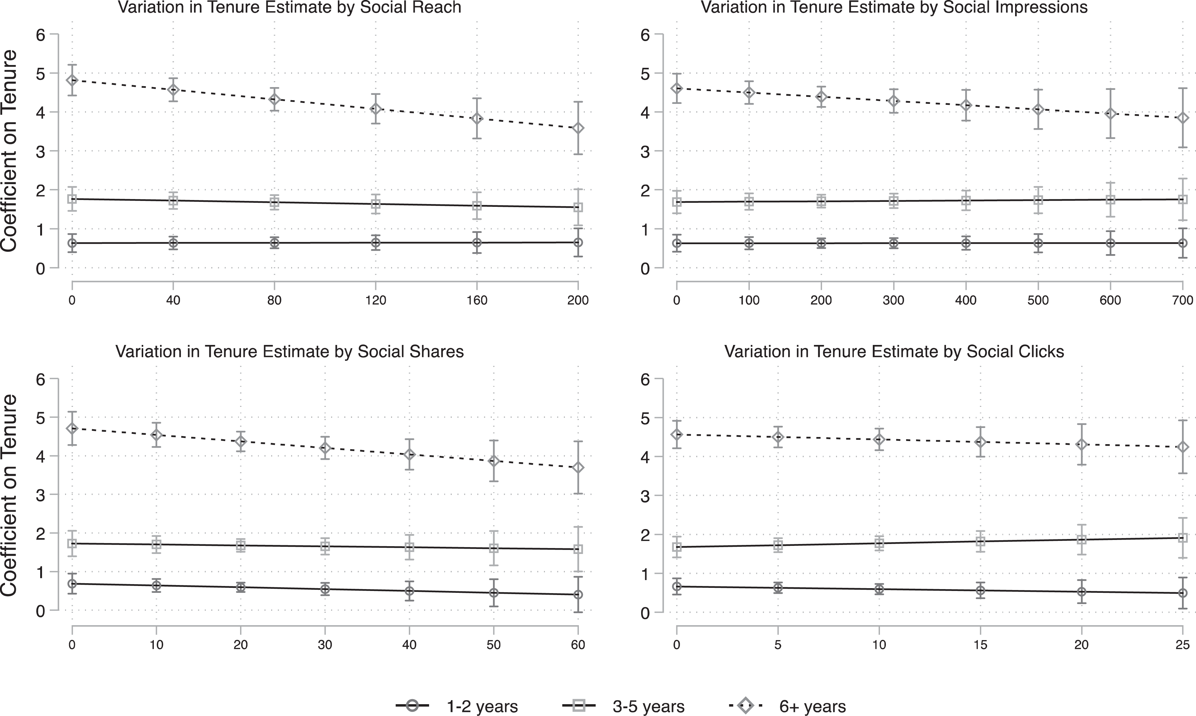
Variation in wage–tenure relationship in shift data by advertisement-level social sharing activity.
While significant, the variation is not large. The estimated return to six years or more of tenure in the preferred pooled models is $4.53. Here, at the lowest levels of social sharing, the estimate is $4.70–4.80, and at the highest levels, it is $3.60–3.70. By way of comparison, the estimated return to six or more years of tenure ranges from $4.96 in the NLSY97 to $3.00 in the CPS. While there is some evidence of bias, the magnitude is substantially less than the difference between NLSY and CPS data sources.
The Value of Firm-level Data: Gender Composition and Wages
The prior section demonstrates how the Shift Project data produce estimates of wages, job tenure, and the relationship between tenure and wages that are broadly consistent with CPS and NLSY data sources and that do not show major bias from unobservables. However, one of the primary rationales for the Shift Project was to collect data at more granular levels, including samples of workers at particular named companies that are not readily available in standard data sources.
To give one illustration of how the Shift Project data on workers at named employers can be used to address research questions that cannot be addressed with existing data, we draw on the large existing literature on how the gender composition of jobs is associated with wages (England 1992). Here, the leading theoretical explanation is that workers in female-dominated jobs are paid less precisely because work that is associated with women is devalued and so less well compensated, even though comparable in terms of job requirements to similar jobs that may be done mostly by men (Levanon, England and Allison 2009; England, et al., 1988). Sociologists, economists, and demographers have amassed a large body of evidence that workers employed in jobs that have larger shares of female incumbents are indeed paid lower wages (England 2005; Levanon et al. 2009; Reskin and Bielby 2005). Notably, this wage penalty is found for both women in female-dominated occupations and for men in such occupations (Budig 2003).
However, this research has, in almost all cases, measured gender composition using occupations or the intersection of industry and occupation (Huffman and Velasco 1997). This source of gender segregation is clearly important for the dynamics of gender inequality in wages. But, there are several other important sources of gender segregation as well. Reskin and Hartmann (1986) point out that in addition to occupational segregation, between-firm gender segregation may importantly shape gender wage inequality—for instance, as men are employed as waiters at fine dining establishments, but women as waitresses at coffee shops. Yet very little existing research has examined the consequences of between-firm gender segregation for gender inequality in wages. Recent work using data from the Equal Employment Opportunity (EEO) Commission examines how managerial gender is related to sex composition within firms (Huffman, Cohen and Pearlman 2010; Kurtulus and Tomaskovic-Devey 2012), but the EEO file lacks data on wages. The work that comes closest to examining how firm-level segregation impacts wages is Tomaskovic-Devey’s (1993) use of a unique 1989 survey of North Carolina employees in which respondents report on the gender composition of their coworkers. Tomaskovic-Devey finds that, drawing on this firm data, the percent female within a job is indeed negatively associated with wages. However, that research is limited to a single state, is more than 30 years old, and relies on a single reporter within each firm to gauge wages and gender composition.
Here, we show how, using the Shift data, we can examine how the gender composition of a relatively homogeneous set of service sector occupations is remunerated and whether this varies by the gender composition of the particular firm. We first generate firm-level measures of gender composition by taking the share of female respondents among all respondents at each of the 38 firms in our data, employing the Facebook weights discussed above. The percent female ranges from 23 percent at Gamestop to 92 percent female at Victoria’s Secret with a mean (median) of 60 percent (59 percent) female across all 38 firms.
We next regress the hourly wage for male and female respondents (pooled) in our data on the gender composition of their employer. In a second model, we introduce controls for demographic and human capital characteristics that could plausibly confound this relationship—age, marital status, race/ethnicity, educational attainment, presence of children in the household, tenure on the job, and managerial status. The relationship between gender composition and wages could though be confounded by nondemographic and nonhuman capital factors. In particular, workers may accept lower wages in return for other compensating job features (Budig and England 2001). In female-dominated occupations, these compensating differentials might be found in work schedules that would be less likely to conflict with care obligations. We control for this source of confounding by measuring work schedule type (regular day, regular night, regular evening, variable, and split/rotating), week-to-week variation in work hours, number of weeks of advance notice, whether the employee works on-call shifts, whether the employee has had shifts canceled, whether the employee has input into his or her work schedule, and a three-item scale measure of work–life conflict engendered by the employee’s job. While measures such as the gender composition of firms are available in the LEHD, it would not be possible to control for this rich set of confounding factors in such administrative data. In a third model, we test whether gender composition is similarly associated with men’s wages and women’s wages (as Budig [2003] finds). Finally, we investigate how the wage returns to tenure that we discussed previously may be moderated by occupational gender composition.
We present the results of these models in Table 3. Model 1 shows the unadjusted relationship between firm-level gender composition and wages and we see a large (−5.69) and statistically significant negative association. In Model 2, we see that, as we would expect, this estimate is substantially reduced after adjusting for worker-level factors to about −2.31 but remains negative and statistically significant. In model 3, we test whether the wage penalty of working at a female-dominated firm is different for male and female workers. The interaction is small and not statistically significant. We then use the estimates in model 2 to plot predicted wages by gender composition in Figure 5. We see that wages at the firms with the smallest share of female employees (Gamestop at 23 percent female) earn about $12.50 per hour as compared with $10.60 at the firm with the largest share of female employees (Victoria’s Secret at 92 percent female). This difference is found after adjusting for the host of individual-level characteristics described above. In plain terms, we find that the mostly female workforce selling women’s underwear make about $2.00 per hour less than the mostly male workforce selling video games.
Firm Gender Composition and Wages.
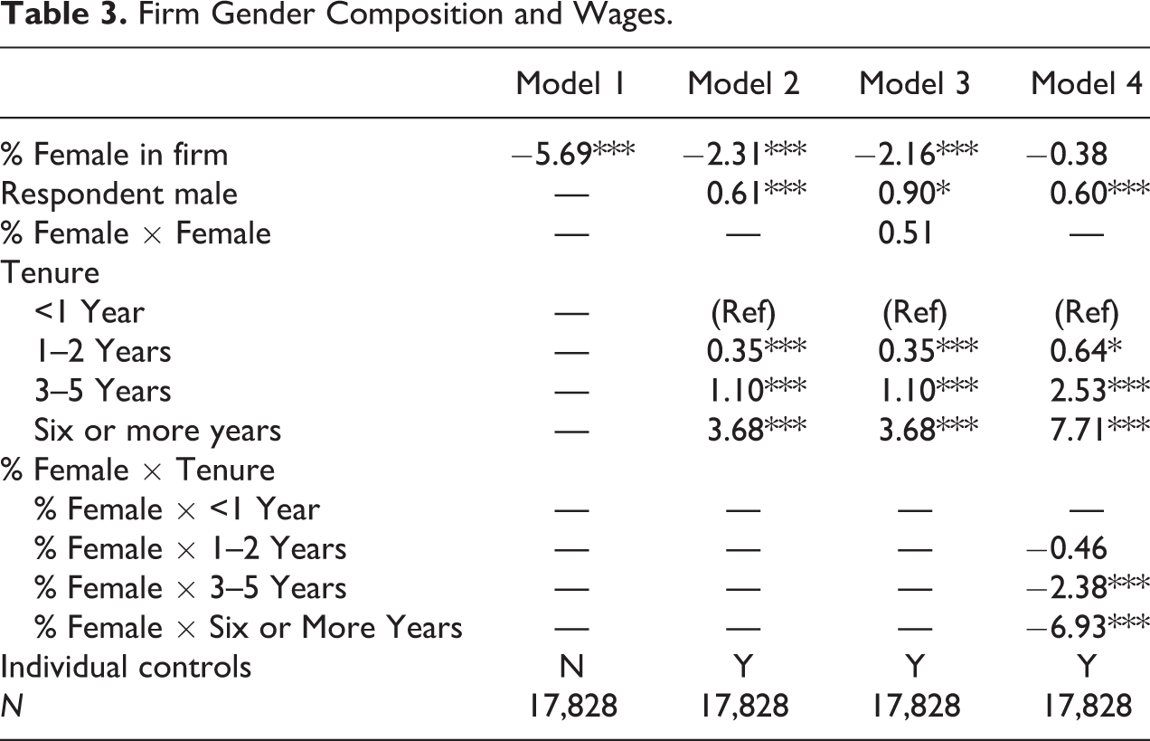
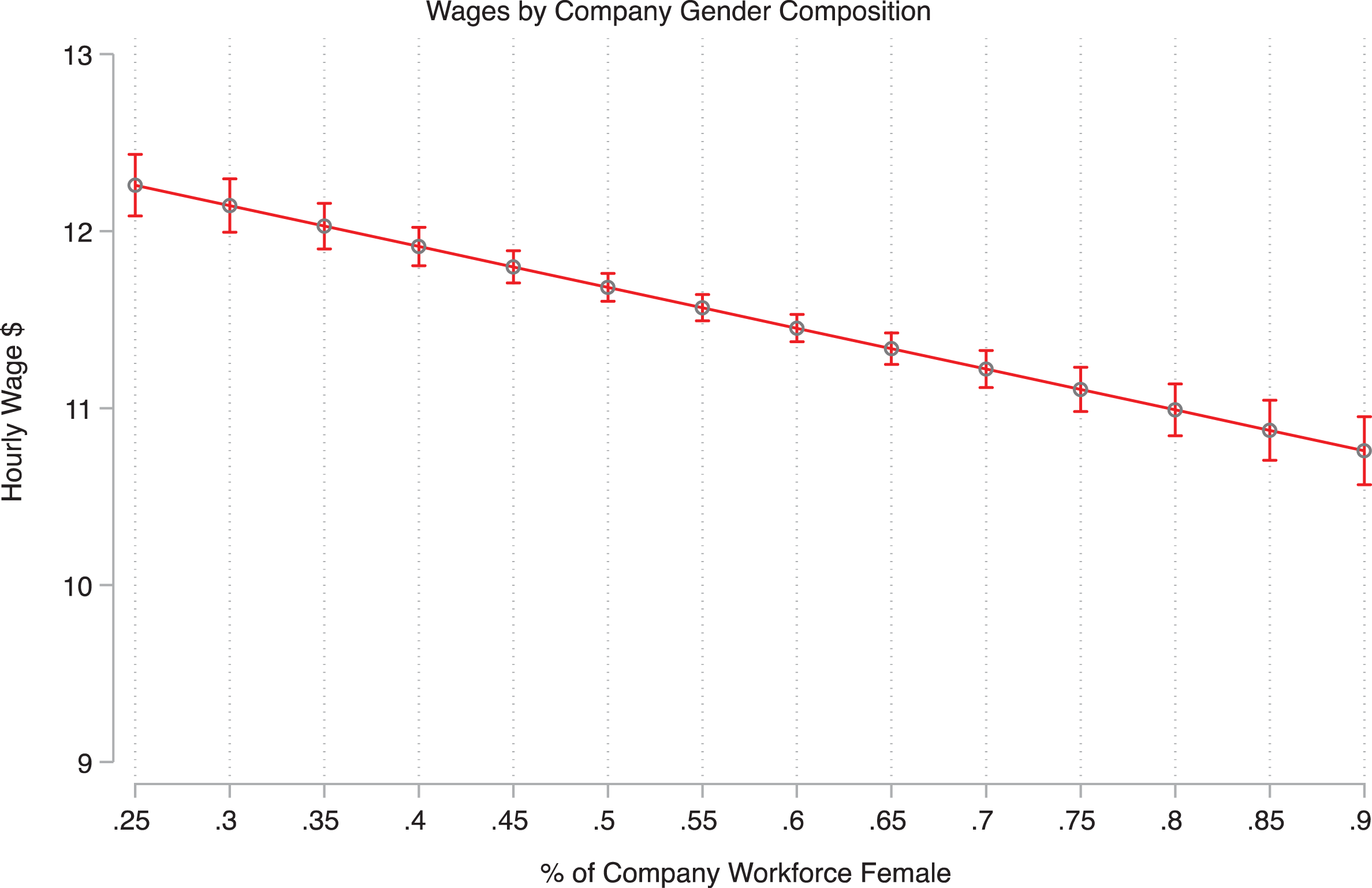
Firm gender composition and wages.
Model 4 provides some evidence for how these between-firm wage gaps take form over time. We see that there is a strong and significant interaction between job tenure and gender composition. We plot predicted wages by years of tenure across the percent of firm employees that are female in Figure 6. It is evident that at the male-dominated firms in our data, there are substantial returns to tenure. Employees with one to two years tenure earn modestly more than those with less than a year of tenure and those with three to five years of tenure do better still. Those with the most tenure, six or more years, see substantial returns to their experience. In contrast, at female-dominated firms, we simply see the absence of a career ladder—the returns to anything less than six years of tenure are nonsignificant and even long tenures of six years or more are associated with only a very modest wage gain. Interestingly, while the returns to three to five and six or more years of tenure are sharply graded, there is little evidence of an association between firm gender composition and wages among recent hires. We also test for interactions with respondent gender and do not find any evidence that these dynamics differ between men and women.
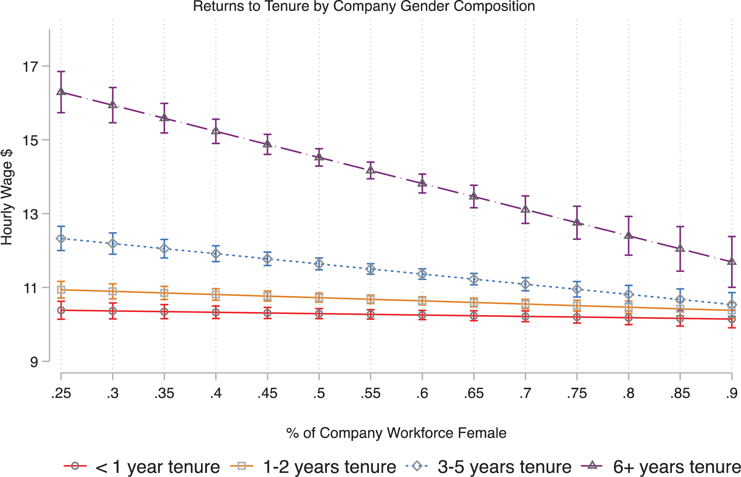
Wage returns to tenure by firm gender composition.
Conclusion
We describe a new integrated approach to nonprobability sampling and survey recruitment that leverages the powerful targeting capabilities of Facebook. Our intervention comes at a time when traditional probability sampling has been declared to be in crisis, beset by low response rates and worsening sampling frames. Important debate and testing continues on the viability of nonprobability online surveys. But, out of this debate, there appears to be an emerging consensus that it remains important to continue to investigate the utility of nonprobability web-based surveys and that such approaches can have real value depending on the research objectives (AAPOR 2010; Schonlau and Couper 2017).
Here, we intervene to try to solve a problem that has long frustrated survey research—to build a sample of respondents, one must have a sampling frame. While researchers have found creative ways to build frames for the general population, it remains very difficult to sample respondents who are nested within organizational entities who may be reluctant or unable to share lists of employees, students, alumni, or members.
While marketers spend tens of billions of dollars a year using Facebook’s targeting tools to try to build brand awareness and sell products to Facebook users, we show that these tools are valuable for survey research as well. We illustrate how targeted advertising on Facebook can be used to build an employee–employer matched data set where hundreds of employees at each of several dozen large firms are recruited and surveyed.
This approach to data collection has several advantages. First, as described above, it provides sampling frames that do not exist (or are very difficult to access) otherwise. Second, it allows for rapid data collection. Third, it is low cost as compared to traditional survey approaches. We also show that these data can be easily weighted to the demographic attributes of similar target populations in such gold standard surveys as the ACS and the CPS, as well as to the eligible population of Facebook users. We then show that respondents in our data resemble respondents in two large and widely used labor force studies—the CPS and the NLSY97—on the key characteristics of wage and tenure. Indeed, there are relatively modest differences in wages and tenure across the two studies and, to the extent that there are differences, the Shift data are no more different from the CPS and NLSY97 than they are from each other. We also show that multivariate relationships—between wages and tenure and wages—are very similar in the Shift data as in the NLSY97 and CPS. On a note of caution, while these comparisons of the Shift Facebook sample against gold standard data sources were reassuring, researchers considering using Facebook or other nontraditional survey recruitment techniques to generate nonprobability samples would be well advised to design and conduct their own comparisons with gold standard or ground truth sources as a data validation check.
Further, we do not suggest that this approach to data collection is without important limitations. First, these tools are likely to be useful to researchers working in other areas where it can be difficult to recruit targeted samples or to access useful sampling frames. However, the approach is particularly well suited to research questions that seek to nest multiple level 1 observations within a set of level 2 units. While our case is companies, scholarship concerned with educational institutions (such as colleges, secondary schools, charters, and so on), military units, neighborhoods, or voluntary organizations might benefit from this approach. The case for using the Facebook approach to assemble national probability sample data seems less compelling because while traditional survey approaches are more costly, sampling frames are readily available. Second, the limitation of using the Facebook approach to construct this sort of hierarchical data is that gold standard probability sample data that would be best used for the construction of weights is, almost definitionally, unavailable. In this application, we have weighted to a similar, but not perfectly well aligned, sample of respondents in the ACS and CPS, but this is a compromise. Third, in traditional survey research, there is a clear connection between the sampling frame and the survey contact. The researcher can determine which phone numbers to call or which addresses to visit. In the case of Facebook, the researcher does not control the processes by which contacts are made from the sampling frame. Instead, Facebook’s advertising algorithm selects which of the eligible users are “contacted” with an advertisement display. This selection process is not publicly described and is subject to change without notice.
Without discounting these important limitations, for the example we illustrate here, these general benefits have tangible results. Because we can inexpensively target employees at a large number of firms, we deploy this method to build an ongoing national monitoring survey of employer management practices and job quality in the retail sector. The ability to rapidly implement a survey and quickly collect data allows us to use these tools to evaluate new local and state ordinances that regulate the employment practices of large retail firms. This speed has allowed us to quickly collect pretreatment data once laws are passed, but before they go into effect. Finally, the ability to collect large numbers of responses from employees nested within firms will permit us to examine how company-level attributes may shape the experience of low-wage work. To illustrate this potential, we estimated the relationship between the gender composition of particular employers and wages, showing that workers employed by service sector employers with a greater share of men in the workforce enjoy higher wages and higher returns to job tenure compared with employers with more female workforces.
Footnotes
Acknowledgment
We gratefully acknowledge grant support from the National Institutes of Child Health and Human Development (R21HD091578), the Robert Wood Johnson Foundation (Award No. 74528), the U.S. Department of Labor (Award No. EO-30277-17-60-5-6), the Washington Center for Equitable Growth (Award No. 39092), the Hellman Family Fund, the Institute for Research on Labor and Employment, and the Berkeley Population Center. We received excellent research assistance from Carmen Brick, Paul Chung, Nick Garcia, Alison Gemmill, Tom Haseloff, Veronique Irwin, Sigrid Luhr, Robert Pickett, Adam Storer, Garrett Strain, and Ugur Yildirim. We are grateful to Liz Ben-Ishai, Annette Bernhardt, Michael Corey, Rachel Deutsch, Dennis Feehan, Carrie Gleason, Anna Haley-Lock, Heather Haveman, Heather Hill, David Harding, Julie Henly, Ken Jacobs, Susan Lambert, Sam Lucas, Andrew Penner, Adam Reich, Jennie Romich, Jesse Rothstein, Hana Shepherd, Stewart Tansley, Jane Waldfogel, and Joan Williams for very useful feedback. We also received helpful feedback from seminar participants at UC Berkeley Sociology, the Institute for Research on Labor and Employment, UC Berkeley MESS, the Washington Center for Equitable Growth, the Institute for the Study of Societal Issues, MIT IWER, UCSF, and UC Davis. This work was approved by the UC Berkeley Committee for the Protection of Human Subjects (2015-10-8014).
Declaration of Conflicting Interests
The author(s) declared no potential conflicts of interest with respect to the research, authorship, and/or publication of this article.
Funding
The author(s) disclosed receipt of the following financial support for the research, authorship, and/or publication of this article: This study received financial support from the National Institutes of Child Health and Human Development (R21HD091578), the Robert Wood Johnson Foundation (Award No. 74528), the U.S. Department of Labor (Award No. EO-30277-17-60-5-6), the Washington Center for Equitable Growth (Award No. 39092), the Hellman Family Fund, the Institute for Research on Labor and Employment, and the Berkeley Population Center.