
Abstract
Quantitative sociologists frequently use simple linear functional forms to estimate associations among variables. However, there is little guidance on whether such simple functional forms correctly reflect the underlying data-generating process. Incorrect model specification can lead to misspecification bias, and a lack of scrutiny of functional forms fosters interference of researcher degrees of freedom in sociological work. In this article, I propose a framework that uses flexible machine learning (ML) methods to provide an indication of the fit potential in a dataset containing the exact same covariates as a researcher’s hypothesized model. When this ML-based fit potential strongly outperforms the researcher’s self-hypothesized functional form, it implies a lack of complexity in the latter. Advances in the field of explainable AI, like the increasingly popular Shapley values, can be used to generate understanding into the ML model such that the researcher’s original functional form can be improved accordingly. The proposed framework aims to use ML beyond solely predictive questions, helping sociologists exploit the potential of ML to identify intricate patterns in data to specify better-fitting, interpretable models. I illustrate the proposed framework using a simulation and real-world examples.
It is common knowledge that valid inference crucially depends on a correctly specified relationship between the outcome of interest,
In the past, simple models like the linear additive functional form were often a necessity due to computational constraints. 1 Yet these historical limitations are no longer a factor, giving rise to ML methods that instead exploit the exponential increase in available computational power. These methods let the data dictate the relationship among variables, rather than relying on the researcher to hypothesize the functional form between the two. 2 Often, this flexibility leads to better-fitting models that improve on researcher-hypothesized models in fitting the data (Brand et al. 2021; Grimmer, Roberts, and Stewart 2021); this has led to increased adoption of ML throughout industry and academia (Athey 2018; Rahal, Verhagen, and Kirk 2022). 3 However, ML methods are almost exclusively applied within a predictive context due to their “black box” nature (Mullainathan and Spiess 2017; Shmueli 2010); their inclusion into sociological inquiry, which has an overwhelmingly explanatory focus, remains limited. 4 This is unnecessary, as the fact that ML methods can identify associations among variables holds value for explanatory work as well.
Concretely, I propose to incorporate ML methods into the typical quantitative empirical workflow in the following way. Assume a researcher is interested in modeling the association between some interest variable and an outcome. To this effect, they apply a conditioning-on-observables approach to control for confounders and develop a hypothesized functional form,
The framework relies on a number of concepts from ML or closely adjacent fields. First, that out-of-sample estimates of model fit can be used to compare the ability of widely varying modeling approaches to fit the data (Rose 2013; Stone 1977; Verhagen 2022). Second, that ML methods can be used as efficient function approximators that can uncover relevant patterns in data (Baćak and Kennedy 2019; Van der Laan, Polley, and Hubbard 2007). Third, that methods from the rapidly evolving field of X-AI—like the Shapley values approach explored in this article that decomposes model predictions along covariates—allow researchers to distill understanding from ML methods, which can then be used to improve hypothesized models (Samek et al. 2019). These elements, in particular the last, allow for an iterative process where ML is used in a supporting role in model-building. The novelty of the framework thus lies in using ML methods as a guide, in such a way that the overarching goal of the framework is still to generate interpretable models (Agrawal, Peterson, and Griffiths 2020; Rudin 2019). This complementary role should be juxtaposed with the overwhelmingly predictive focus of ML methods in sociology up until now (Molina and Garip 2019). The framework is also in line with increasing calls to use ML in a supportive role throughout the empirical pipeline, rather than completely replacing interpretable methods for ML equivalents (Agrawal et al. 2020; Rudin 2019; Rudin et al. 2010).6,7
Incorporating ML and X-AI methods into empirical work should not only improve model-building but also improve transparency into the research process. A lack of emphasis on functional form specification provides researchers with relative freedom in evaluating multiple functional forms and choosing which one to report (Muñoz and Young 2018; Sala-i Martin 1997; Simonsohn, Simmons, and Nelson 2020). Such “researcher degrees of freedom” are to blame for a large number of important empirical findings turning out to be un-reproducible and a more general “crisis in science,” where results are often dependent on over-engineered models (Gelman and Loken 2013; Ioannidis 2005; Young 2018). Comparing a researcher’s carefully tailored model to the fit of an ML method estimated to the same data can help identify such an over-engineered model, by providing insights into model fit that are not a result of a researcher’s decision-making process but rather a feature of the data. More generally, overfitting is a central concern throughout ML, and the frequent re-estimating of models on subsets—standard practice throughout ML—can further protect against “p-hacking” (Gelman and Loken 2013).
More generally, the proposed framework provides a welcome realignment of empirical methods with today’s computational reality (Efron and Hastie 2016) and is in line with increasing calls for a re-appreciation of the predictive power of social theories that can be observed more broadly throughout sociology (Hofman, Sharma, and Watts 2017; Verhagen 2022; Watts 2014, 2017).
The rest of this article is structured as follows. I first introduce a toy example to illustrate the risk of model misspecification to inference. Then, I introduce the three steps of the proposed framework and illustrate each by applying them to the same toy example. I next compare the proposed approach to other computational frameworks. In the empirical section, I apply the framework to one simulated and two real-world case studies. In doing so, I illustrate how the framework identifies (1) missing nonlinearities and interactions in a simulated dataset on the association between schooling and earnings, (2) nonlinearities and spatial heterogeneity in a large dataset on London house sales, and (3) various intricate patterns in voting preferences among U.S. voters in the General Social Survey (GSS).
Misspecification and Risks to Inference
Consider the following toy example. Our interest lies in whether having grandchildren affects elderly individuals’ worries about climate change. We analyze a survey

which simply plugs all the relevant controls and our interest variable into a linear additive model. We might also consider including a nonlinearity in the effect of age by adding a square (Model 2):

Results for estimating both models on a simulated dataset are presented in the first two columns in the left-hand panel of Table 1. We find a substantial difference between the two models in terms of the estimated association between having grandchildren and concerns with climate change. The effect is statistically insignificant for Model 1 with a point estimate of −0.02, whereas it is negative and significant
Table on the left shows regression results when estimating a functional form assuming linear age, quadratic age, and a step function for age; Plot on the right shows implied effect of age for the three model specifications.
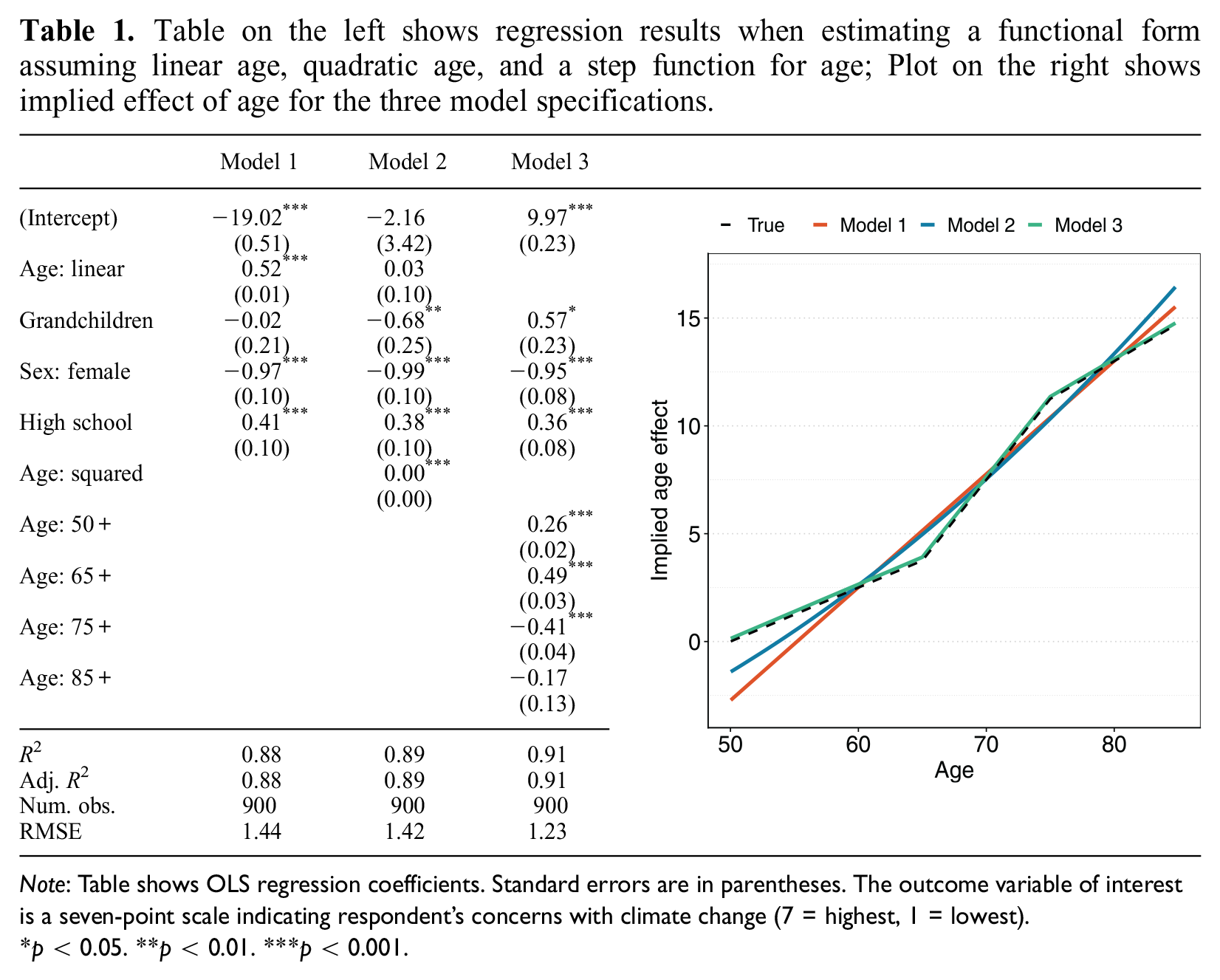
Note: Table shows OLS regression coefficients. Standard errors are in parentheses. The outcome variable of interest is a seven-point scale indicating respondent’s concerns with climate change (7 = highest, 1 = lowest).
p < 0.05. **p < 0.01. ***p < 0.001.
Imagine, however, that the true effect of age is indeed nonlinear, but piece-wise linear rather than a second-degree polynomial. Specifically, there is a stronger increase in concern by age among people age 65 to 75, with more modest increases at other ages. If we had estimated a functional form in line with this nonlinearity, we would find results as reported in the third column of the left panel of Table 1. These results show that the effect of having grandchildren is in fact associated with a higher level of concern. The estimated age effect per functional form is illustrated in the right panel of Table 1, with the dashed line representing the “true” effect in the DGP and the colored lines the best-fitting effect given the flexibility of the model. The problem is that both the linear and the quadratic function of age overshoots the true effect as the respondent’s age increases. Coupled with the fact that grandchildren are more prevalent among the older population, this effect leads to incorrect inference.
The issue with doing inference into the first two models is that the assumption of exogeneity, that is,
Implied association from a linear model (dashed line) relative to the true effect (solid line).
Various statistical tests have been proposed to combat misspecification. The most popular ones are White’s test for functional misspecification (White 1980, 1981) and Ramsey’s RESET test (Ramsey 1969). White’s test statistic is based on a comparison of the estimated coefficients from a hypothesized model
First, they are generally under-powered and can struggle to identify misspecification in multivariate settings (Buja, Kuchibhotla, et al. 2019:616). 11 Second, they provide limited insight into what to do next, if a test is rejected. Third, and perhaps most important, the actual implementation of misspecification tests is limited in published empirical work (Long and Trivedi 1992; Open Science Collaboration 2015). As a case in point, the two flagship journals in sociology—the American Sociological Review and American Journal of Sociology—totalled 70 research articles in 2022. Of these, 40 included quantitative analyses, of which 32 implemented a conditioning-on-observables approach. None of these articles implement any of the standard misspecification tests like the White or RESET tests. 12 In practice, researchers enjoy relative freedom in specifying their functional form, as well as the robustness and specification tests they use to verify its appropriateness. The crisis in reproducibility and the effect of researcher degrees of freedom on empirical results thus extends to the (lack of) specification checks chosen by researchers to validate their model assumptions (Simonsohn et al. 2020; Young 2018).
Even without malicious intent, many functional forms are from an outdated age of computational limitations (Buja, Kuchibhotla, et al. 2019:615; Efron and Hastie 2016; Muñoz and Young 2018). The linear additive functional forms plugged into exponential family probability distributions were historically preferred due to their ease of estimation and interpretation, not their de facto appropriateness to study social life. This pragmatic preference for parsimony has led to the continued prevalence of simplistic functional forms, even though the computational constraints under which they were developed are no longer present, and the wealth of qualitative research in the social sciences consistently implies that social life is in fact highly complex and probably not appropriately modeled using such simple functional forms (Abbott 1988). As the toy example above illustrates, inference can easily go astray given the often blind acceptance of simplistic functional forms in empirical work.
A Computational Framework to Improve Model-Building
I propose a computational framework that exploits ML methods to obtain an indication of the potential model fit in a dataset. This potential can then be compared to the fit of a researcher’s own hypothesized model, and thus used to diagnose a possible lack of specification in the latter. This estimate provides researchers with an intuitive assessment of how well the data could be modeled versus how well the data is modeled by their hypothesized model. ML thus takes a guiding role in model-building. Whenever it is found that the ML model improves on the researcher-hypothesized model, methods from the X-AI domain can be implemented to unpack and better understand the ML model and subsequently improve the hypothesized model.
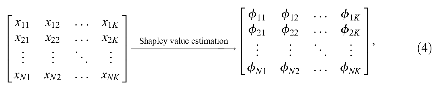
Given a dataset
Estimate hypothesized model
Evaluate the model fit of both
Diagnose why
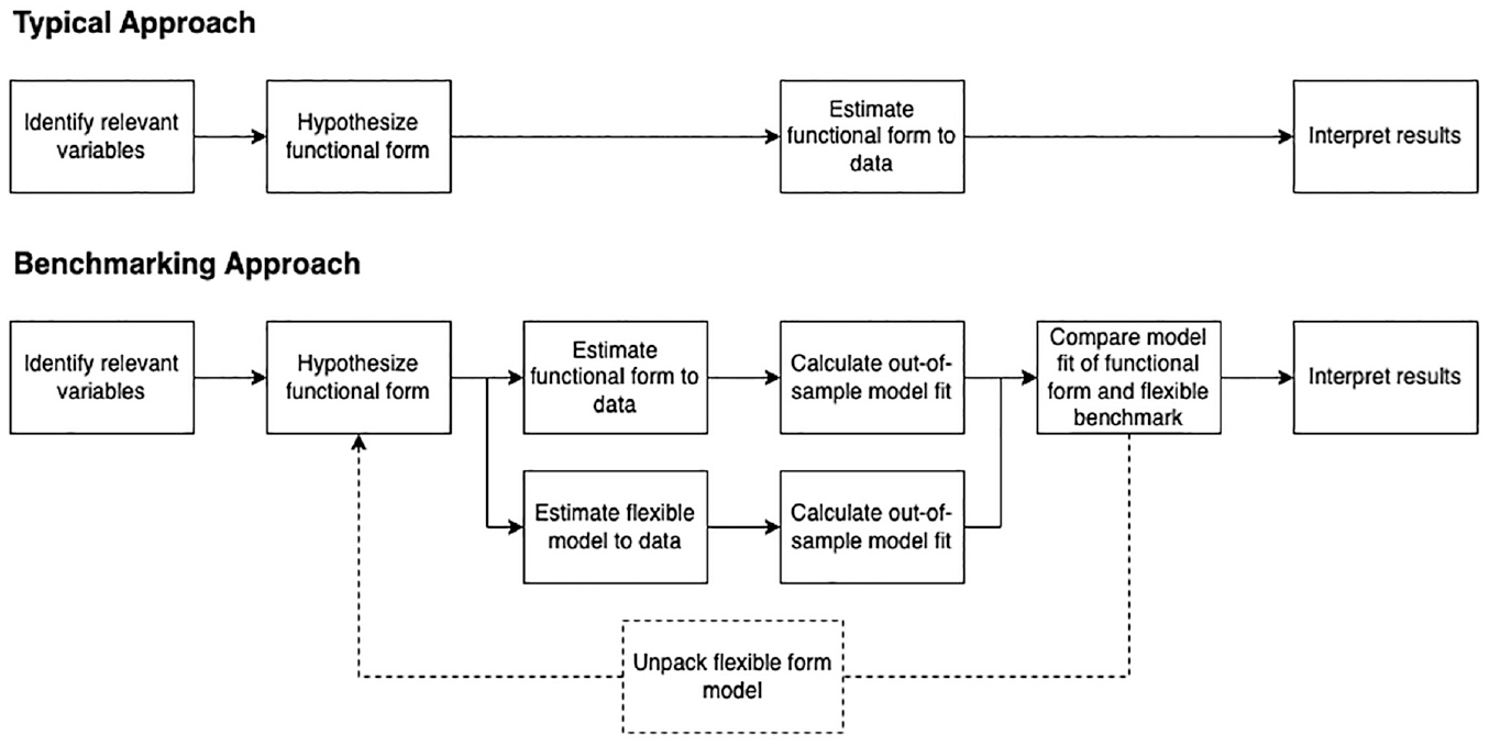
Schematic illustration of the proposed framework.
Crucial to the framework is that the ML method is estimated using the same variables as present in the model originally hypothesized by the researcher. The framework is not designed for data-mining, where a large number of possible explanatory variables are included in the model. In such a case, one risks including variables that might improve model fit but could harm understanding of the underlying processes—typical examples would be (accidentally) including post-treatment variables or colliders. Instead, the functional form is scrutinized given the exact same inferential curation of variables and logic as present in the researcher’s originally hypothesized model. 13 The following sections describe the three components of the proposed framework in more detail and illustrate them using the toy example.
Step I: The benchmarking model
The first component of the proposed framework is a flexible form model
Many different ML methods can be applied to datasets commonly encountered in the social sciences (Athey 2018; Hastie, Tibshirani, and Friedman 2009). In fact, limiting the benchmarking step to a single researcher-curated ML model to serve as
The Super Learner is an example of such an ensemble method, consisting of multiple ML methods or the same method with different parameter settings. Among these, the most appropriate model is identified using cross-validation. The oracle result by Van Der Laan and Dudoit (2003) shows that a Super Learner is indeed optimal to identify the best-fitting model to approximate an unknown DGP among evaluated models, and the price of including large numbers of models into the Super Learner is minor in terms of performance (Baćak and Kennedy 2019; Van der Laan et al. 2007; Van der Vaart, Dudoit, and van der Laan 2006). Therefore, many models can and should be evaluated, and ensembles of various methods are typically preferred as function approximators over single models (Agrawal et al. 2020). 14 A Super Learner can also be specified prior to model estimation and preregistered, improving transparency in the research process (Open Science Collaboration 2015). Naturally, the full set of models and the resulting fit of each should be part of the research output. 15
Among the broader set of ML methods, some approaches lend themselves better than others to modeling social science data (Chen and Guestrin 2016; Lundberg et al. 2020). In particular, tree-based methods deal well with various types of data often encountered in the social sciences (e.g., categorical and numerical variables) and can handle missing data. They also do not require exponential increases in sample size as the feature space increases. Furthermore, the most popular tree-based methods, like the Random Forest (RF) or Gradient Boosting (GB) model, require relatively little tuning on the part of the researcher and can be applied out-of-the-box or with limited effort to most social science datasets (Breiman 1996; Freund and Schapire 1996).
16
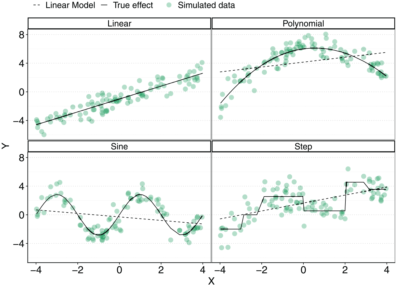
These advantages make tree-based approaches an attractive class of ML methods to include in the benchmarking step. As a case in point, consider the nonlinear associations in Figure 3, which were introduced earlier. As before, the black lines illustrate true associations and the green diamonds are a hypothetical dataset generated by the true association and some white noise. The blue dots and red squares are out-of-sample predicted values based on a GB and an RF model trained to 80 observed data points and fed with 100 uniformly distributed
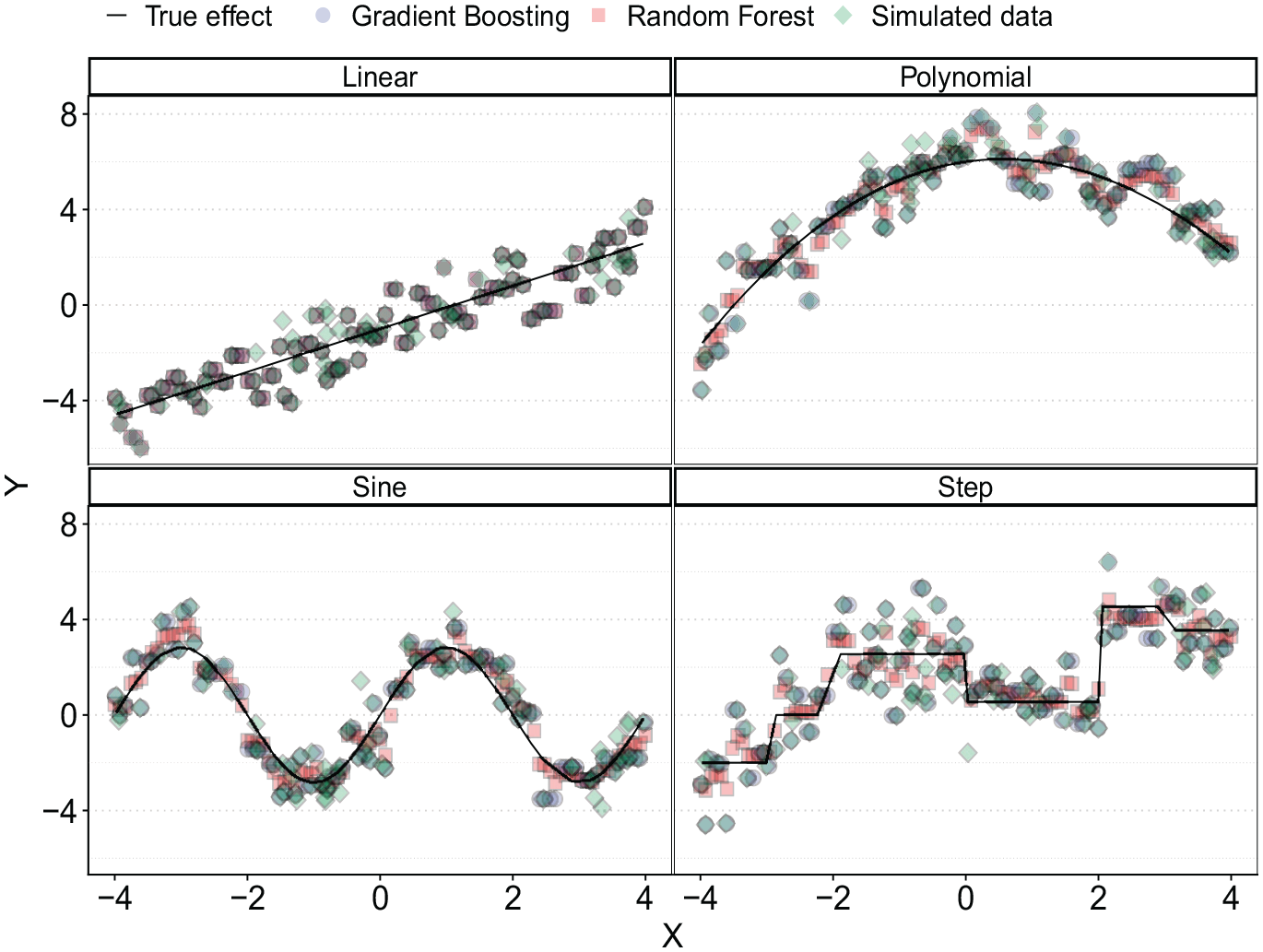
Predicted outcome using a GB (blue dots) and RF (red squares) model fit to noisy data (green diamonds).
I illustrate the first step of the framework by estimating a Super Learner including a number of GB and RF models with various parameter estimates to the toy example introduced earlier. I also include the two researcher-hypothesized models to the Super Learner, reflecting the model including linear (
Truncated Super Learner Performance Using the Toy Example Data.
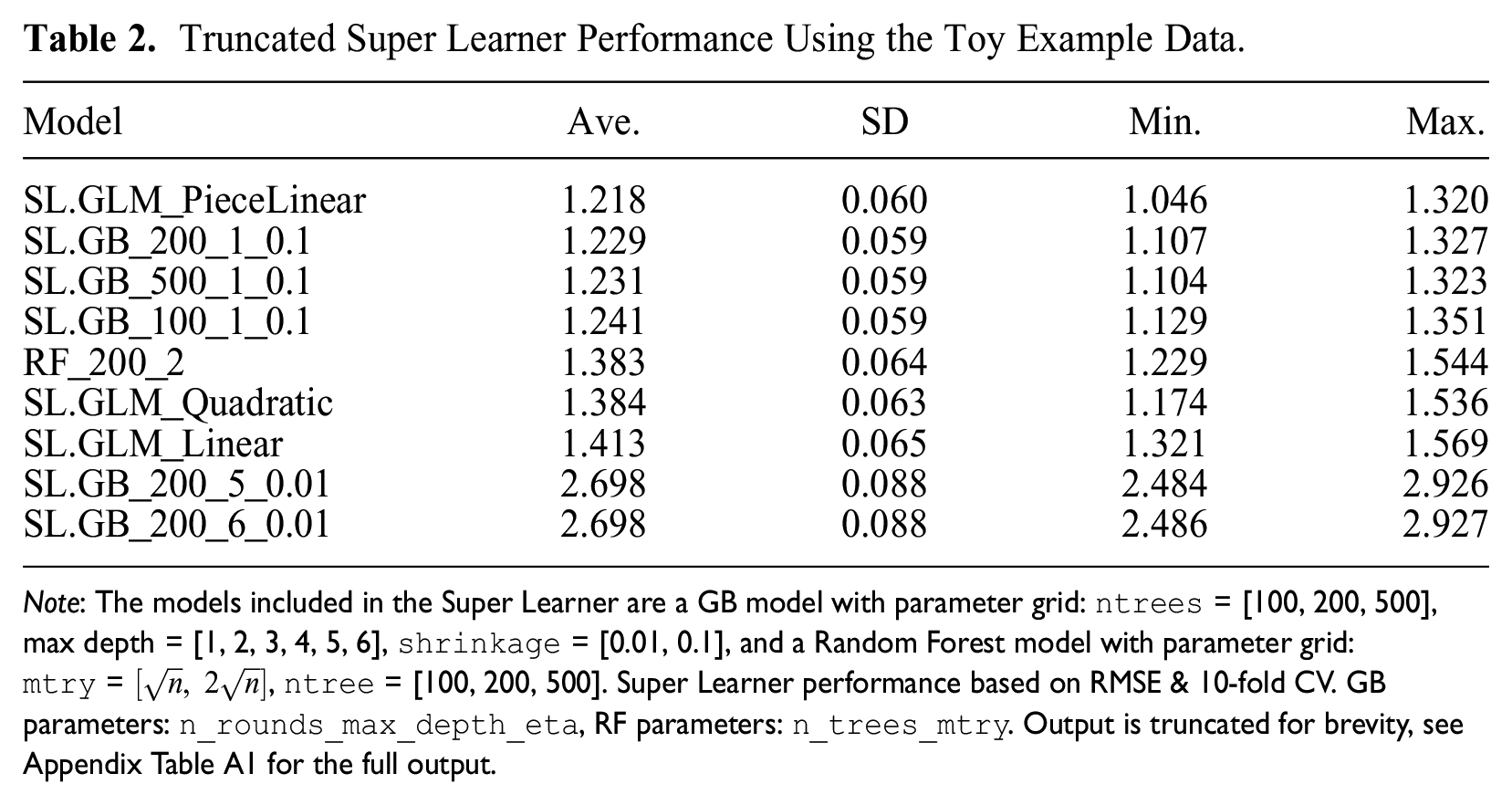
Note: The models included in the Super Learner are a GB model with parameter grid:
Step II: Estimating and comparing model fit
The second component of the proposed framework is a metric to compare the fit of benchmarking model
Formally, the out-of-sample estimation of model fit would require splitting the total dataset
As others have noted, fit need not automatically equate with the best model from an inferential perspective (Grimmer et al. 2021; Muñoz and Young 2018). This discussion is often concerned with including colliders or post-treatment variables in a model, or simply including as many variables as a researcher can possibly think of. Such practices typically improve fit, but they can invalidate inference. This is the central reason why the proposed framework uses the same inferential reasoning in terms of which explanatory variables are included in the flexible model as the originally hypothesized model. Much of the criticism regarding blind “fit-hunting,” where all causal or inferential logic is effectively abandoned in favor of model fit, is thus not applicable, and variable selection is driven by the substantive question rather than fit (Grimmer et al. 2021:412). 21 However, it can be challenging to identify when a difference in fit between the flexible and researcher-hypothesized model warrants a re-evaluation of the latter. For example, improvements in fit for a covariate uncorrelated with the interest variable may have little bearing on the consistency of the interest variable. 22 Ideally, we would like clear statistical guidance on the extent of bias in an underspecified model. In practice, the decision to unpack the flexible form model will likely depend on the willingness of both the researcher to defend a specification with an apparent lack of fit, and the research community to accept it. This is not a consequence of the framework, but a level of uncertainty resulting from embracing a state of the world where we acknowledge that we have very little knowledge about the true DGP and are unwilling to make stringent assumptions on it a priori.
Putting the second step of the framework into practice, I compare the model fit of the GB model identified in Step 1 with the two hypothesized alternatives for the toy example. I include two fit metrics: the R-squared
Three linear additive models and a GB model estimated on a train set consisting of 80 percent of the total dataset.
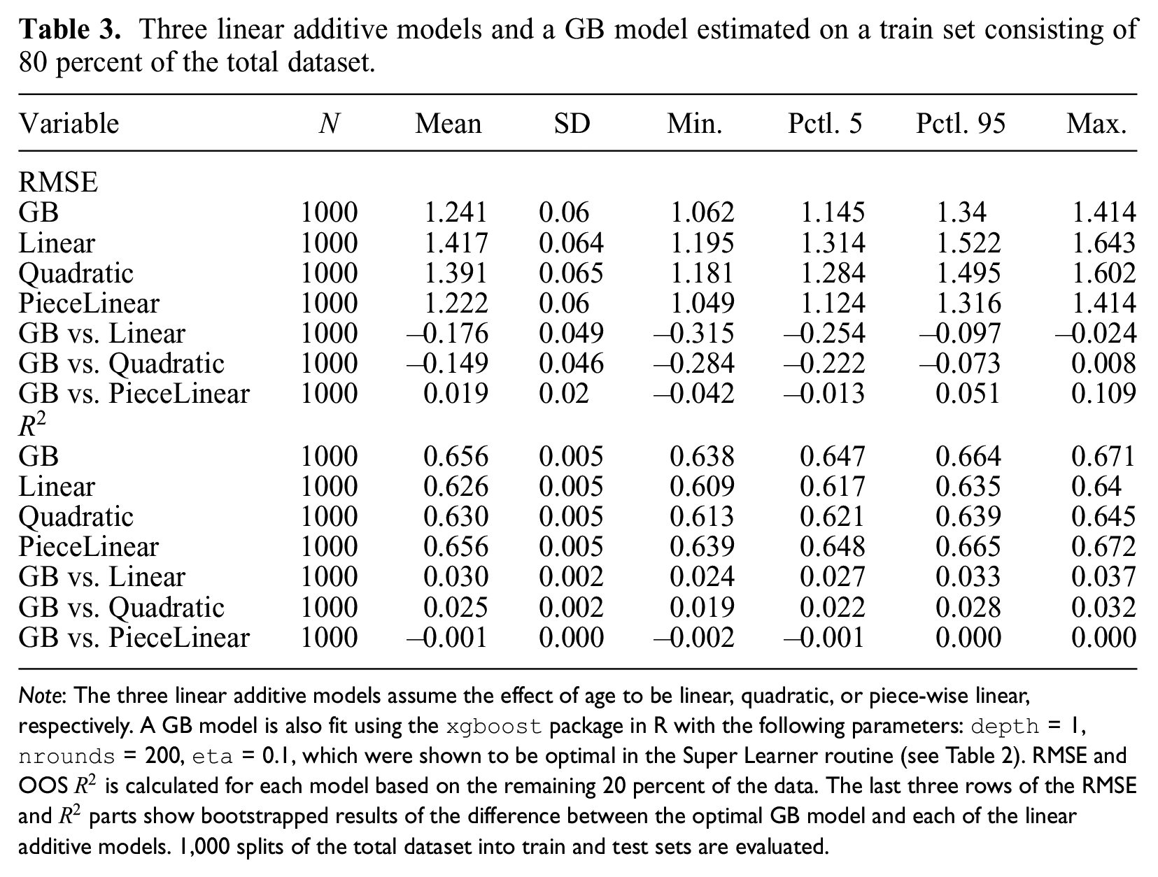
Note: The three linear additive models assume the effect of age to be linear, quadratic, or piece-wise linear, respectively. A GB model is also fit using the
Step III: Unpacking the ML model
The third and final component of the proposed framework is a method to generate understanding of the ML model whenever it outperforms the hypothesized model in a way that warrants re-evaluation of the originally hypothesized functional form. The increasing application of ML models in everyday life has led to pressure to improve understanding of the inner workings of ML models. 24 These developments have led to the emergence of X-AI, which focuses on understanding the patterns underlying ML models. Two general approaches can be identified within X-AI: global and local explainability. The former attempts to describe the mechanics of a model in general terms, that is, which variables tend to be important for the model’s overall performance. The reporting of variable importance measures are an example of this approach (Baćak and Kennedy 2019; Brand et al. 2021). In local explainability, the goal is to explain the drivers of singular predictions made by a model. Local explanation methods are more appropriate for the framework, as they provide insights into the actual functional patterns between covariates and the outcome.
Various local explanation methods have been developed for different substantive questions that may be asked of a model (Doshi-Velez and Kim 2017; Lipton 2018; Zhou et al. 2021). 25 For example, much explainability research is focused on providing additional ad-hoc context into a model’s predictions for practitioners making (high-stakes) decisions. In such cases, the ability to quickly calculate and extract information underlying a model’s prediction could be more relevant than emphasizing fidelity. Conversely, an ethical reviewer of a system-in-action might require more fine-grained and detailed explanations. Within the proposed framework, the onus is on understanding the underlying patterns found by the ML model, rather than any practical or regulatory concerns. This motivates the use of Shapley values, which have a number of unique and attractive properties with extensive theoretical grounding (discussed in more detail below). 26 Importantly, recent advances have made their estimation computationally feasible and rekindled a general interest in their use (Aas, Jullum, and Løland 2021; Heskes et al. 2020; Samek et al. 2019). Shapley values also align closely with human intuitions of model interpretation, making them appropriate for the iterative process envisioned in the framework (Doshi-Velez and Kim 2017; Lundberg and Lee 2017; Rudin 2019). Shapley values have been applied in various fields, notably medicine (Lundberg et al. 2020; Tang et al. 2021), but have also found applications in sociological research, for instance, as a way to understand complex network dynamics (van der Laan et al. 2022) and to resolve path dependencies in decomposition metrics like segregation indices (Elbers 2023).
Shapley values for model explanation
Shapley values were originally developed within cooperative game theory to assist in the task of distributing a game’s overall payout to its participants. Because a game’s payout can depend on its participants’ actions in a potentially complex manner, such an attribution function is not trivial to determine—for instance, some players’ participation may have no bearing on the outcome at all. Shapley (1953) developed a perturbation-based approach to determine such an allocation mechanism for games of arbitrary complexity that possesses various attractive theoretical guarantees.
When used for model explanation, every single prediction
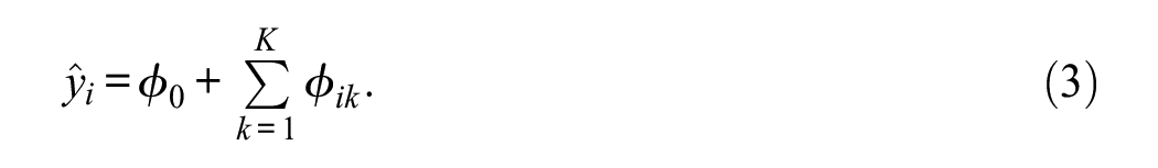
Here,
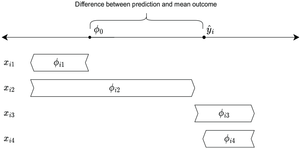
Prediction
As every single prediction
where all
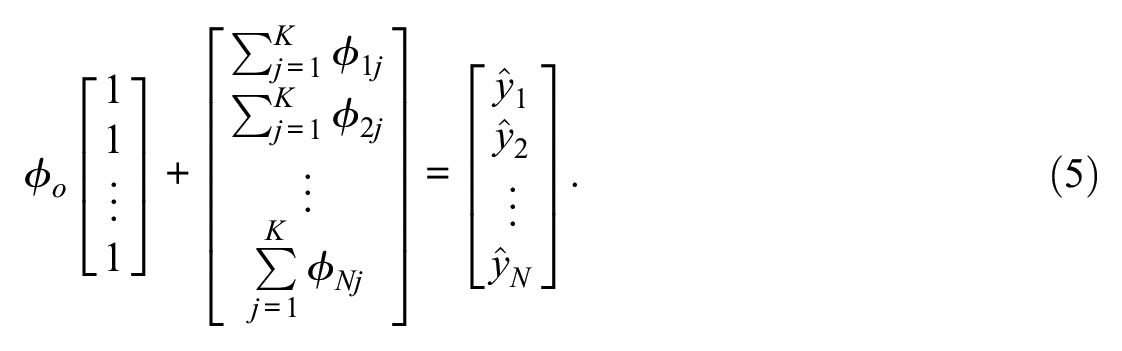
Note that if the model was a standard linear additive model without an intercept (i.e.,
The process of calculating the
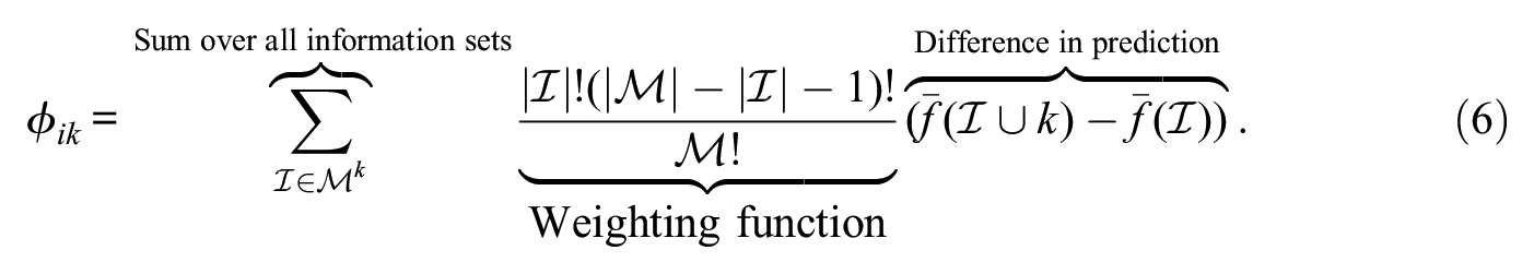
This process is then repeated for every variable
Shapley values have a number of unique theoretical properties that make them attractive as a method to generate understanding of models. First, the sum of all Shapley values
The computational burden of calculating Shapley values stems from three elements. First, the number of possible information sets is
Tree SHAP exploits the structure of the estimated tree, allowing for a much smaller set of relevant information sets to be assessed. Specifically, information sets that only differ from one another in terms of variables that do not feature in the branches of the tree can be ignored, as they will not lead to different predictions.
28
This has made estimation efficient to the point that exact Shapley values can be calculated, rather than having to rely on numerical approximations (Lundberg et al. 2020:64–65), and even renders pairwise Shapley values feasible to calculate in reasonable time (Lapuschkin et al. 2019; Lundberg et al. 2020). Pairwise Shapley values assess the joint omission of two variables from the model and the subsequent effect on the outcome, allowing interactions to be explicated. In the standard Shapley decomposition in Equation 3, interactions would be divided among the relevant interacting variables.
29
A final benefit of the Tree SHAP approach is that the independence assumption when making expectations for those variables outside of the information set,
To illustrate how Shapley values can be used to generate understanding into an ML model, I calculate all
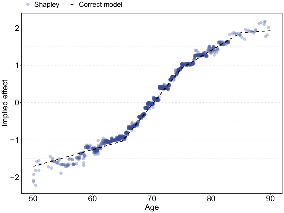
Implied effect size of age through Shapley values versus the correctly specified model.
Resemblances to Other Computational Frameworks
Before applying the framework to three empirical cases, I briefly discuss a number of methods and frameworks that share a similar intuition and computational appetite to the proposed framework. In spirit, the first two steps of the framework are indebted to modern types of specification tests that rely on comparing residuals from classic non-parametric regression to those provided by a researcher’s own hypothesized model. 31 Such approaches can identify a broader range of nonlinear functional forms than those considered by the RESET test, for example, although formal tests of improved fit remain challenging to compute due to the dependence of local estimates to the data at hand. More generally, the amount of data required to compute such local estimates scales exponentially with the number of independent variables (Bishop 2006; Yatchew 2003). The ML methods proposed for the framework presented here retain considerably more structure and are more efficient from a data perspective than non-parametric tests are, improving efficiency and allowing for better post-estimation analysis. 32
The proposed framework also shares similar goals to the field of model robustness. The emphasis in model robustness lies in exposing the potential role of researcher degrees of freedom during the model-building process (Sala-i Martin 1997; Simonsohn et al. 2020; Young 2019). A large number of “plausible” models are estimated that slightly differ to the hypothesized model to guard against researchers cherrypicking a specification. The key difference in model robustness is that variation is typically induced by excluding variables in the model, rather than assessing different functional relationships among variables (Young and Holsteen 2017). 33 The functional complexity and the fit of the models is of limited importance (Slez 2019; Young 2019). The proposed framework instead focuses on the functional relationship among a set number of variables and the emphasis is on specification. 34 Both approaches could be combined by applying the proposed framework to different sets of explanatory variables, as I will illustrate in two empirical case studies. Despite their differences, both frameworks are similarly indebted to the growth in computational power that allows researchers to consider many different functional forms and to use these computational riches to be more critical of modeling assumptions and improve transparency into the research process (Muñoz and Young 2018:4). 35
Closest in spirit to the proposed framework is an emerging literature in behavioral economics and psychology using ML models to find the predictive limit of behavioral theories (Agrawal et al. 2020; Kleinberg, Liang, and Mullainathan 2017; Peterson et al. 2021). The typical approach is to compare the performance of some behavioral theory to predict the outcomes of a stylized experiment (e.g., the fairness perception of two vignettes [Agrawal et al. 2020]) with a flexible ML model trained to the same data. If the ML method leads to better predictions than a behavioral theory, cases where the behavioral theory underperformed relative to the ML benchmark are studied. This research focuses solely on large-scale experimental data and has not been extended to empirical work as broadly as I propose here. The onus in this literature is on theory completeness rather than correct functional form specification. Post-estimation interpretation of the ML method—the third step in the proposed framework—is mostly ad hoc, if present at all. 36 However, the central premise of using ML to find patterns in data not necessarily hypothesized by a researcher is a key similarity between the two approaches.
A final strand of research similar to the proposed framework is the field of “autometrics,” which also aims to find better-fitting models than a researcher’s own hypothesizing might yield. The autometrics approach includes a large number of base transformations of the explanatory variables into a linear additive functional form. This “stacked” model is then iteratively trimmed to reach an optimal model using in-sample fit metrics and specification tests (Doornik and Hendry 2015). Autometrics is a more classical approach to flexible model-building compared to the ML methods proposed here. Specifically, the autometrics setup can be subsumed by the set of ML methods called “generalized additive models” and spline-based methods, which can be folded into Step I of the proposed framework (Hastie and Tibshirani 1987; Hastie et al. 2009). 37 Related, scholars have put forward similarly stacked models that include interactions but then apply variable selection through least absolute shrinkage and selection operator regression (Blackwell and Olson 2022; Beiser-McGrath and Beiser-McGrath 2020). The proposed framework shares the same general intuition of the above approaches but uses a broader set of methods such that a wider range of patterns can be identified, and it emphasizes out-of-sample evaluation to reduce the risk of overfitting and path dependence in eliminating regressors from the model. As with all frameworks mentioned here, the inclusion of the third step in the proposed framework is another key difference with the above approach.
Applying the Framework in Practice
I apply the proposed framework to three case studies. The first is a simulation based on the Mincerian wage equation, a classic field of research investigating the returns of additional years of schooling on a person’s income (Lemieux 2006). The second is a hedonic regression of house prices applied to a large dataset of transactions in the London retail market (Malpezzi 2003). The third is a study of the demographic determinants of voting preferences in the United States using the General Social Survey (GSS) (Davis and Smith 1991). The Mincerian wage application is relevant because it provides an example of a functional form that has been actively innovated upon over the past decades and illustrates how the proposed framework can speed up model-building. I chose the hedonic regression and voting examples because both enjoy considerable academic interest, and models typically include a number of standard control variables with a (novel) interest variable. Because the latter is often correlated with the control variables, a correct functional relationship is crucial for inference. For these latter two case studies, I evaluate whether the typical complexity in which control variables feature in the functional form is sufficient, and improve them where necessary. Across these cases, I identify various nonlinearities and interaction effects using the framework. 38
Application I: Mincerian wage simulation
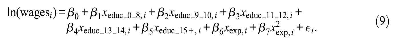
The Mincerian wage equation is a classic economic tool used to estimate the effect of an additional year of education on an individual’s wages—the “return to education” (Lemieux 2006). As mentioned above, the Mincerian wage equation has been actively innovated upon over the past decades. In the original functional form, log yearly wages was related to years of education and work experience in a linear additive fashion:

Subsequently, a square term was added to allow for a level of nonlinearity in the effect of work experience:

More recently, a step function was added in the effect of education to allow for different linear effects by level of education:
For illustrative purposes, I also study a fourth, hypothetical functional form where each coefficient slightly differs by sex:
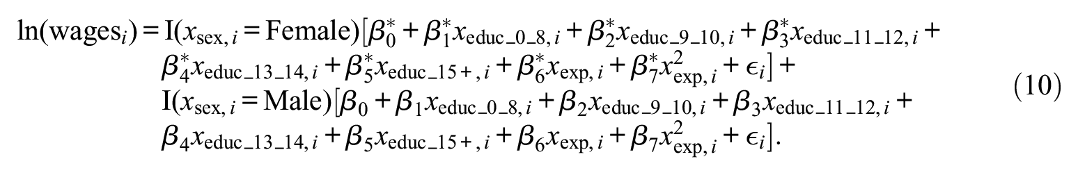
To illustrate the proposed framework, I simulate data using the four specifications above as DGPs, plugging coefficient estimates as found in the recent empirical literature into each specification. For the final specification, I vary the coefficients of sex to fall within a standard error of the coefficients found in the literature (see the Appendix for the DGPs) (Heckman et al. 2018; Lemieux 2006).
Based on these four DGPs and a synthetic sample of 50,000 individuals’ age, years of education, years of work experience, and sex, I generate four outcomes: one using each DGP. The synthetic sample is based on the GSS 2018, such that the distribution of the explanatory variables is representative of an actual working population. For illustrative purposes, I calibrate the error term in each functional form such that the proportion of explainable variance is constant in every dataset irrespective of the DGP used to generate the outcome variable. Descriptives for the dataset can be found in Appendix Table A2. Linear-I refers to the first functional form above provided by Equation 7, Linear-II refers to Equation 8, and so on.
The above leads to four datasets consisting of a distinct vector of outcomes
In addition to the four hypothesized functional forms, I estimate a Super Learner including various tree-based ML methods—the first step of the framework. A GB model performs best for each of the four datasets (see Appendix Tables A3 and A4). In the second step of the framework, I compare the model fit of the flexible model with the four hypothesized models using Monte Carlo cross-validation. The results show that the flexible model is able to match the true functional form’s performance in the first three datasets and strongly outperforms the most flexible functional form in the fourth dataset (see Figure 6). The framework thus identifies the underlying model without requiring the researcher to hypothesize a functional form in all four datasets.
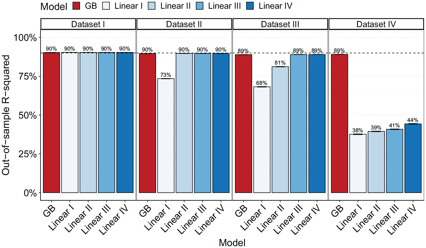
Out-of-sample
Finally, the flexible model can be unpacked to infer why it improved on the hypothesized functional forms—the third step in the framework. We know the true DGP in this case, making it obvious why the flexible model outperformed the underspecified functional forms, but the Shapley values easily identify the correct association of the independent variables with the outcome (Figure 7). The Shapley values capture the linearity of both explanatory variables in the first dataset, the nonlinearity in years of work experience in the second dataset, and the step-wise function in the third dataset. The Shapley values also pick up the interaction with sex in the fourth dataset, as illustrated by varying the Shapley values by sex. Clearly, assuming linearity where none is present leads to a misrepresentation of the true returns to education; incorporating the correct flexibility is crucial for inference.
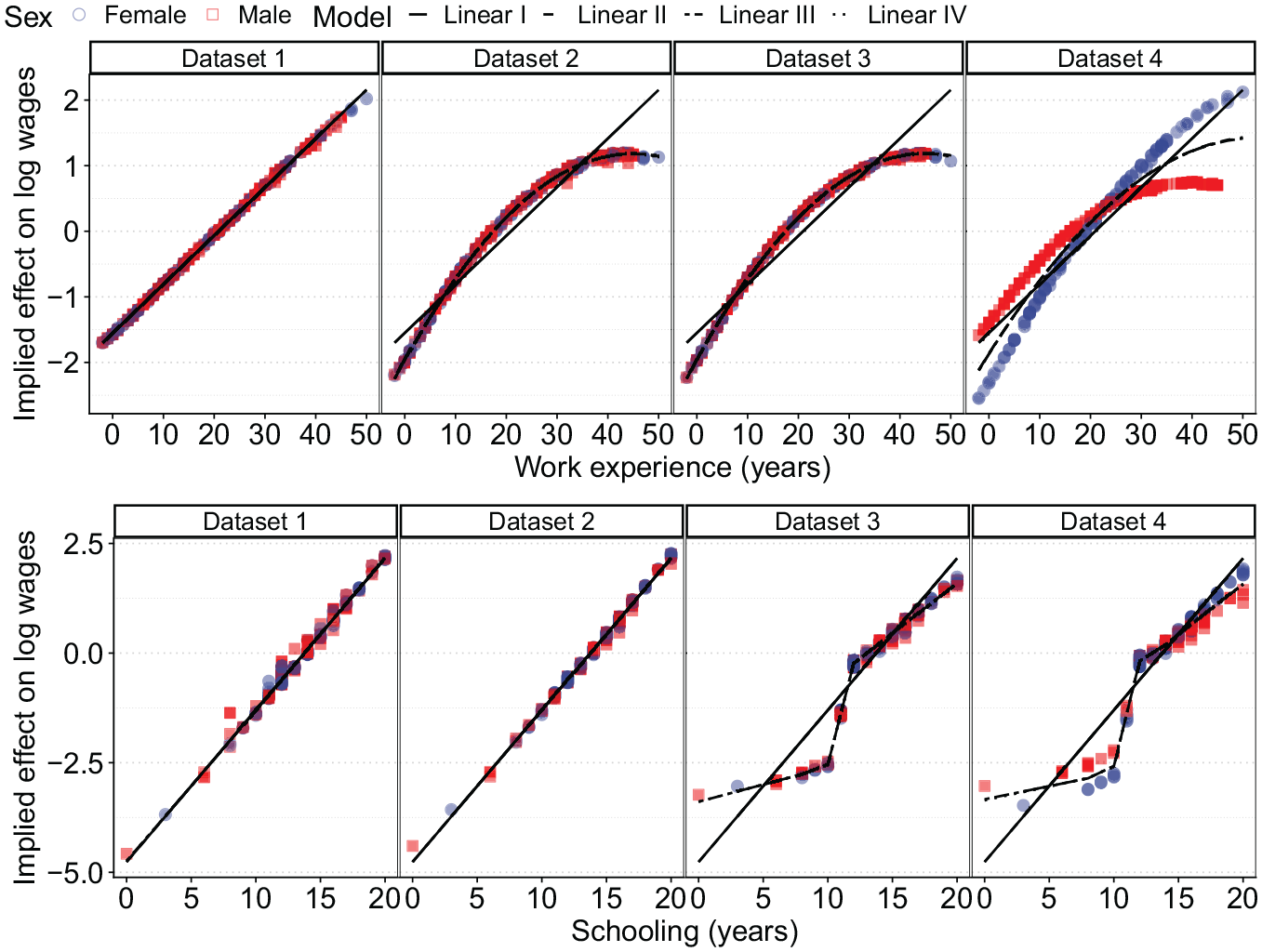
Effect of work experience (red squares) and schooling (blue circles) as predicted by the four estimated functional forms, and as implied by Shapley values.
Application II: London house prices
As a second case study, I use a large dataset on transactions in the London housing market. The typical approach to modeling house prices is through a hedonic pricing model that assumes each house is composed of various traits for which buyers have certain preferences. Buyers effectively combine the value of individual traits to determine the (monetary) value of an entire house. In hedonic regression, interest typically lies in the price elasticity of certain traits, for example, how much the house price increases with an additional square meter of living space or the inclusion of a garden. In practice, linear additive models are typically estimated relating observed house characteristics with log prices, although many authors have suggested that the assumptions of additive linearity implicit in this functional form might be unreasonable (Fan, Ong, and Koh 2006; Malpezzi 2003).
In this application I use typical house characteristics, like house size, number of rooms, and property type as explanatory variables. I also include a number of neighborhood characteristics. In many applications, researchers attempt to address spatial heterogeneity by including neighborhood-level observables like crime indices, travel distances to local centers, or deprivation scores. Again, in the typical model these variables are added in a linear additive framework, although it is often argued that spatial heterogeneity is considerably more complex (Elhorst 2010). To estimate the hedonic regression, I use a dataset of nearly 630,000 house sales containing basic house characteristics and a neighborhood identifier. The transaction data were collected and merged by the Reshare project hosted at the UK Data Service (Chi et al. 2021). I include neighborhood-level data from the Department of Transport and Communities and Ministry of Housing, Communities and Local Government. 39 I also include the year and month of the transaction. Descriptive statistics of the dataset are shown in Appendix Table A5.
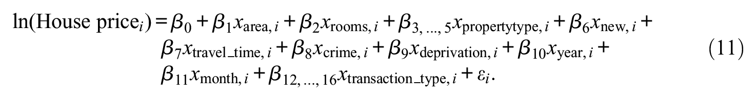
For the hypothesized model, I estimate a linear additive functional form relating log house prices to the variables depicted in Appendix Table A5. As is customary in the literature, I assume linear trends for all continuous variables, including the temporal variables. The exact functional form is as follows:
Following the framework, I start by estimating both the hypothesized model and a Super Learner to the data. In addition to the model in Equation 11, I also apply the framework to subsets of the full model. The best-fitting flexible model is again a GB approach, which will be used as the flexible model (see Appendix Tables A6 and A7 for the Super Learner output for the full set of covariates, and the selected models for the covariate subsets, respectively). In the next step, the fit of the flexible model is compared to the hypothesized model. The results are summarized in Figure 8 and are striking. Already among the simplest housing characteristics, like size and property type, the flexible model improves on the linear additive functional form by about 5 pp in terms of the out-of-sample
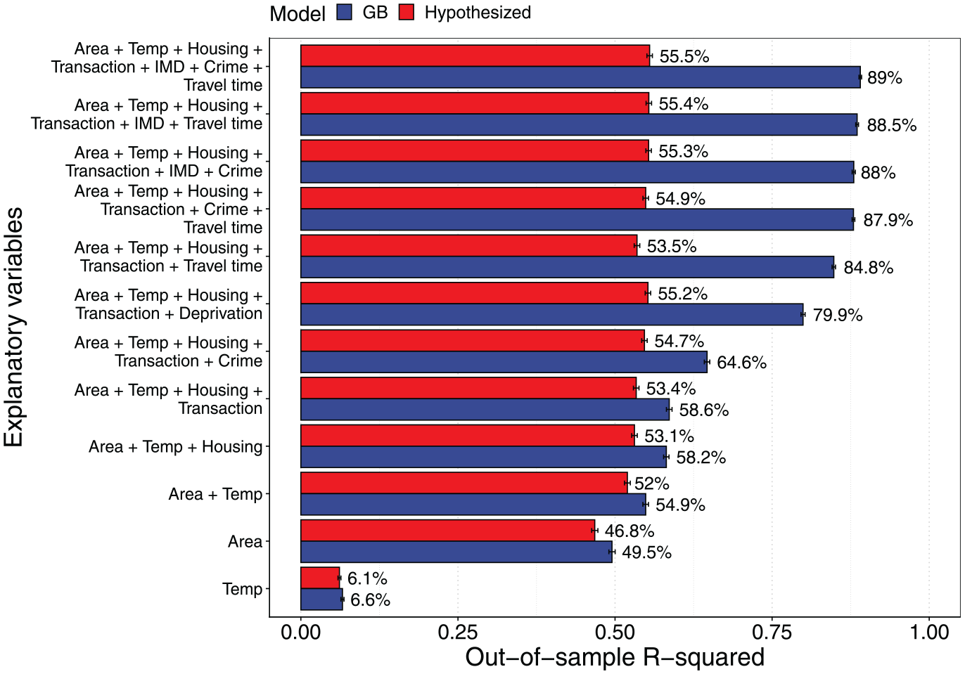
Out-of-sample
To evaluate why the flexible model outperforms the linear additive framework, I calculate Shapley values for the flexible model. These are visualized for six explanatory variables: the size of the house, the travel time to the nearest local hub, the crime index, number of rooms in the house, and the two temporal variables (year and month of sale). Figure 9 shows the results. We see nonlinearities for most of these variables, ranging from a slightly decreasing elasticity for the size of the house to piece-wise linearity in the effect for travel time and the crime index. It is also clear that the number of rooms, year, and month variables should all be modeled in a nonlinear way. When including these nonlinearities into the linear additive model, the fit improves and is strictly preferred according to an LR test, 40 although a remaining gap in model fit still points at further interactions and nonlinearities among variables, possibly across time. Specifically, the considerable noise in the Shapley values of the neighborhood-level variables implies that these variables do not follow a very precise pattern with respect to the neighborhood characteristics, and including nonlinearities may not suffice to capture the underlying patterns well.
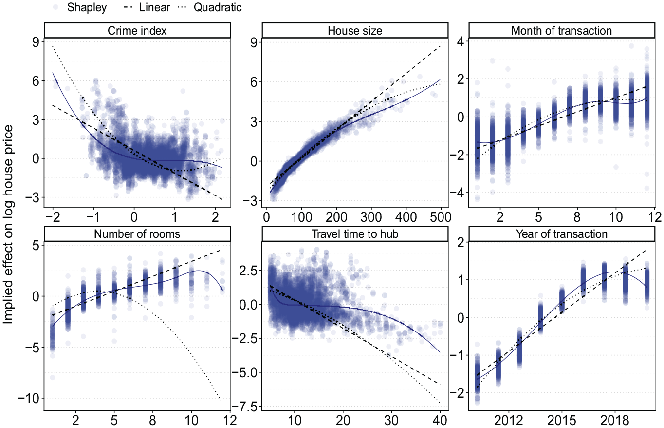
Plots show implied effect from a typical linear additive model (dashed line), when adding a squared term (dotted) and as implied by Shapley values (scatter).
Given the stark increase in model fit when adding neighborhood-level variables, I include random intercepts on the neighborhood level to a simple model including the house size and temporal explanatory variables. This effectively provides a fully nonlinear association for each neighborhood’s characteristics and the outcome variable, which seems reasonable based on the large increases in model fit when adding any of the neighborhood characteristics to the flexible model, combined with the variation in their Shapley values. Based on this modification of the functional form, the out-of-sample
Application III: Party identification in the United States
As a third and final case study, I evaluate the demographic determinants of party identification in the United States using the GSS (Davis and Smith 1991). Party identification is of substantive interest in the social sciences (Freeden, Sargent, and Stears 2013), and the GSS is an often-used resource for this purpose. Throughout this literature, a number of demographic variables are used as typical controls, including respondent’s age, sex, race, educational attainment, and income. Another variable of substantive interest is usually included in the analysis, like cognitive ability (Meisenberg 2015) or social class (Morgan and Lee 2017). These interest variables naturally tend to correlate with the control variables, making correct specification critical.
Appendix Table A8 shows descriptive statistics of the GSS containing information on voting preferences and demographic characteristics between 1974 and 2018. The outcome of interest is a seven-point scale indicating whether the respondent identifies strongly with the Democratic party (value of 1) or the Republican party (value of 7). The GSS also includes the respondent’s age, years of schooling, income level across 12 brackets, sex, and race, as well as the year of the survey wave. As the hypothesized model, I use a standard linear additive model as often encountered in the literature (Freeden et al. 2013). Most functional forms include a linear time trend for the year of the survey, and add most demographic variables as a linear determinant or dummy. The hypothesized functional form is as follows:
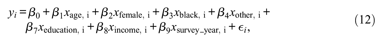
and resembles that found in Meisenberg (2015).
I start by estimating Equation 12 as well as a Super Learner containing various tree-based ML models using both the full set of covariates and subsets. The best-performing model is again a GB model, although the RF also performs well (see Appendix Tables A9 and A10 for the Super Learner output for the full set of covariates, and the selected models for the covariate subsets, respectively). Figure 10 shows results from benchmarking the out-of-sample
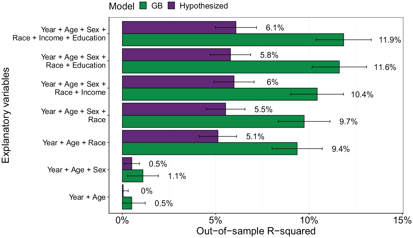
Out-of-sample
Using the full set of covariates, Figure 11 illustrates Shapley values and Shapley interaction values for the age, schooling, and income variables. These Shapley values show there are clear nonlinearities in the associations of age, income, and years of schooling with the outcome. Assuming these associations to be linear does not fit the implied effect well, and adding square terms improves the model fit considerably (Figure 11A). 41 Ignoring these complexities and assuming a linear functional form would wrongfully imply a decreasing effect by age, even though there is a clear upward association at later ages. Similar incorrect conclusions would be drawn for both the education and income associations when assuming a linear additive model.
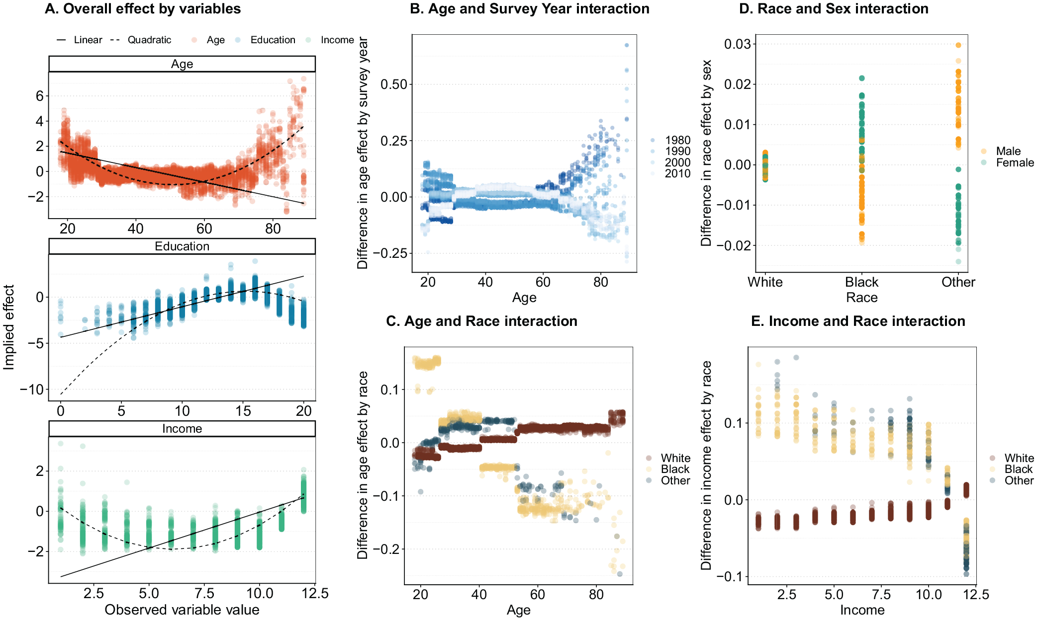
Overall implied effect as estimated by Shapley values for age, education, and income variables: (A) overall effect by variables, (B) age and survey year interaction, (C) age and race interaction, (D) race and sex interaction, and (E) income and race interaction.
These direct effects can be further decomposed into a number of interactions by estimating pairwise Shapley values, allowing each Shapley value to be decomposed into a direct and indirect effect. The indirect effects indicate how Shapley values for certain observed characteristics deviate from the overall effect of the variable, conditional on a second variable. The estimates in panels B to E all show indirect effects and illustrate that younger respondents associated less strongly with Democrats in earlier waves than in later waves (Figure 11B), but also that White individuals have a stronger positive age effect than do non-White individuals (Figure 11C). We see similarly interesting dynamics when interacting sex and race, which show that the sex effect is more pronounced for Black respondents but is less pronounced for others (Figure 11D). The effect of income shows similarly complicated dynamics, where higher income is associated more strongly with Republican identification for White individuals than for non-White individuals (Figure 11E). Adding race interactions for sex, income, and age as implied by the Shapley values improves the fit of the hypothesized model using conventional in-sample fit statistics. 42
Discussion
This article set out to address a key problem in quantitative sociology: that we do not know what the appropriate functional form might be to model a dataset. In addition, a historic preference for parsimonious and easy-to-estimate models due to computational limitations has led to researchers hypothesizing relatively simplistic functional forms with little scrutiny. Not only does this lead to risks of misspecification bias and incorrect inference, but a lack of emphasis on appropriate specification can lead to researcher degrees of freedom muddying empirical findings. I argue that instead of trusting researchers to conjure up the correct functional form, we should use methods that embrace the fundamental uncertainty regarding the underlying patterns in a dataset to help sociologists improve their model-building.
I proposed a framework using ML methods to generate a data-driven estimate of the fit potential in a dataset. This fit potential indicates how well an outcome could be modeled when the functional relationship among variables is dictated by the data. Such an estimate provides an indication of whether a researcher’s own functional form might miss important nuances like interactions or nonlinearities. Crucially, the fit potential is a feature of the data and not a result of the researcher’s choices, improving transparency in the empirical process. Whenever the ML method finds more intricate patterns in the data than our own models do, we can unpack the former to provide guidance on how to improve the latter. This is contrary to popular belief that ML models are fundamentally black boxes that cannot convey any intuition into the patterns they identify. More generally, the proposed framework provides a bridge between the ability of ML methods to identify intricate patterns in data and a desire for interpretable models. By incorporating existing methods into the standard empirical workflow, ML models become complementary tools in the sociologist’s empirical toolkit, as opposed to the near exclusive use of ML for predictive questions, as is the status quo in sociology.
Illustrating the framework, I showed how the historic process of model-development could have been sped up considerably, using the example of the Mincerian wage equation. The framework effortlessly identified underspecification, and subsequent analysis of the ML models identified the necessary improvements to the functional form. The other two empirical examples, a hedonic regression of house prices and a model explaining party identification, both illustrate how often-encountered modeling strategies lead to considerably lower fit than does a flexible ML model. In the case of house prices in London, a number of simple nonlinearities were identified. Most importantly, the fundamental inability to address spatial heterogeneity through the inclusion of standard neighborhood characteristics became clear through the considerable differences in fit between the hypothesized and ML method when including neighborhood data. For party identification, a lack of complexity was similarly evident from applying the framework, and unpacking the flexible models showed important interactions and nonlinearities between the explanatory variables and outcome, which are not commonly implemented in the functional forms used to study party identification.
Existing misspecification tests have known limitations, but appropriate use would have identified a lack of specification in some of the examples presented in this article. 43 However, classic misspecification tests are known to be underpowered, especially in multivariate settings, and limited in the types of misspecification they consider. Fully non-parametric tests are more flexible, but suffer heavily from the curse of dimensionality. In addition, misspecification tests do not provide clear guidance on how to improve a functional form after misspecification is identified. Perhaps most importantly, use of even the most basic of misspecification tests is practically nonexistent in sociological work, and its selective implementation can suffer from the very same researcher degrees of freedom they are meant to address. Conversely, the only source of selectivity in the proposed framework is what models to include in a Super Learner to provide an estimate of the fit potential. As the price of considering a large amount of models is small, this risk is minimal and we can simply include a large amount of different types of methods. In contrast to classic misspecification tests, the proposed framework also provides researchers with concrete guidance into the type of patterns that may have been missed.
The approach presented here also has limitations. First, uncovering intricate patterns will still depend on the available data and might provide limited guidance in low
Perhaps the most challenging part of the framework is determining how much improvement in fit is enough to warrant a re-evaluation of the functional form. Unfortunately, this question will fundamentally depend on a combination of the substantive research question being asked and the true underlying DGP. As a result, the choice to accept a functional form will likely remain a debate among the academic community. This is not so much a consequence of the framework, but rather one of embracing the fact that we know very little about the true DGP and are unwilling to make stringent assumptions on it, nor blindly trust that a researcher-hypothesized model includes all the relevant intricacies in the data. A result of increasingly letting go of assumptions regarding the underlying DGP will be that we are left more frequently with questions like the one posed above, where we can rely less on statistical guidance and will instead have to rely on academic discussion.
At the root of most empirical sociological findings lies a functional form that is assumed to be correctly specified. Limited evaluation of whether this functional form is appropriate for the data leads to a number of serious risks. The model might not accurately reflect the patterns in the data, affecting the validity of statistical inference. Simply allowing researchers to report a single or curated number of functional forms without much scrutiny further exposes sociology to p-hacking. These practices stem from a time when limitations on computational power necessitated parsimony. These constraints are no longer applicable, yet the models we estimate retain a simplicity that likely belies the intricacies of the social mechanisms we are interested in. This is evidenced in the work of our qualitative colleagues, as well as the ever-increasing number of empirical examples where ML models outperform the linear additive models usually estimated by sociologists. I proposed a framework to address this issue by exploiting the benefits of ML methods—to find intricate patterns in data—to address this key issue throughout empirical work. This symbiosis of quantitative sociological work and the computational riches of today is long overdue, and it will only bear more fruit as the goals of the ML community increasingly align with the explanatory focus of sociologists.