Beyond Proximity: Investigating Crime With Organic Neighborhoods and a Two-Stage Unsupervised Learning Approach

Abstract

Studying the relationship between neighborhoods and individual-level outcomes such as crime, labor market success, or intergenerational mobility has a long history in the social sciences. As local processes like gentrification constantly change neighborhoods’ composition and spatial expansion, time-constant one-size-fits-all neighborhood measures fail to capture important local dynamics. This article presents a flexible and data-driven approach for efficiently estimating overlapping and arbitrarily shaped neighborhoods with time-dynamic boundaries. Constructed in a two-stage clustering design, the first stage identifies homogeneous groups within a city, while the second stage clusters homogeneous groups by spatial proximity. In an analysis of 86 million person-year observations from 76 German cities, the paper shows that a larger spatial expansion of affluent neighborhoods negatively correlates with city crime cases, while higher neighborhood fragmentation and heterogeneity correlate positively with crime rates. The findings stress the importance of flexible neighborhood estimation techniques and the necessity to view neighborhoods as nonconstant entities.

Introduction

Research on the relationship between neighborhoods and individual-level outcomes such as criminal behavior (Levy et al. 2020; Light and Thomas 2019; Mayer and Jencks 1989; Sampson et al. 1997), labor market success (Clampet-Lundquist and Massey 2008; Jahn and Neugart 2020), or intergenerational mobility (Chetty and Hendren 2018) has a long history in the social sciences. While quantitative studies have provided important evidence on how certain types of neighborhoods benefit or harm individuals, mostly qualitative or segregation studies have documented that not only time but also individuals’ own characteristics affect the spatial expansion of perceived neighborhood boundaries (Coulton et al. 2001, 2013; Kye and Halpern-Manners 2022; Rich 2009; Schelling 1971; Shedd 2015). Due to data limitations, these two strands of neighborhood literature have long coexisted.

With the rise of computational social science and new data capabilities, researchers have adopted new quantitative neighborhood approaches such as egohoods, that is, actor-centered “neighborhood” buffers (Hipp and Boessen 2013), or enhanced network approaches that capture the subjective social reality in neighborhoods better than previous predefined aggregate measures. Typically based on interaction data from smartphones or surveys, network-based neighborhood approaches generate neighborhoods of arbitrary shapes and sizes by exploiting that most interactions are local (Hipp and Perrin 2009; Poorthuis 2018). However, network approaches do not have a genuine spatial component like other spatial aggregation approaches. Therefore, network-based neighborhoods can neither directly account for spatial distance nor capture neighborhood components being independent of interaction. Moreover, the limited data availability and high computational intensity of network approaches have prevented their widespread use and time-repeated estimations. As (perceived) neighborhood boundaries are often contested (Legewie 2018) and even likely to change over time (Logan 2012; O'Sullivan 2009; Rey et al. 2011), time-repeated estimations are crucial for understanding local dynamics and contextual effects by adding a time-varying component to neighborhood analysis.

Contributing to the literature on neighborhoods, this article presents a computationally efficient and data-driven aggregation approach for constructing organic neighborhoods with time-dynamic boundaries and different sizes and shapes. These social or “organic neighborhoods” (Legewie 2018: 1959) not only capture the social reality of their residents better but also have less demanding data requirements than comparable network and deep learning approaches. Designed as a two-stage clustering approach, the approach relies on similarity between residents as a baseline condition while keeping spatial proximity as the main neighborhood dimension. To do so, the first stage identifies homogeneous groups within a city (using an automated K-Means algorithm), while the second stage clusters these homogeneous groups by spatial proximity (using a hierarchical density-based clustering algorithm, called HDBSCAN; McInnes et al. 2017). Unlike previous neighborhood measures with constant area size and boundaries, the proposed two-stage approach produces overlapping organic neighborhoods with different sizes, shapes, and densities. Moreover, the data requirements are less demanding than for network approaches, since the input data ideally consist of georeferenced point data, but also work with larger spatial units such as grid cells. By allowing the area size and boundaries to change over time, the approach can track processes of neighborhood evolution and fragmentation for the first time. Finally, the approach is less computationally intensive and more transparent than comparable neural networks, Bayesian, or regression approaches.

In investigating the relevance and added value of organic neighborhoods compared to aggregate population characteristics (e.g., average income or unemployment of a city) for sociological research, the second part of the article is a proof-of-concept application to city crime. I follow the notion of social disorganization theory (Kornhauser 1978; Sampson and Groves 1989; Shaw and McKay 1942) and generate organic neighborhoods based on socioeconomic status (SES) using individual-level administrative data. Social disorganization theory explains how a neighborhood's aggregate level of SES, the residential heterogeneity, and the neighborhood's temporal stability affect local criminal activities (Sampson and Groves 1989). For the years 2000 to 2017, I use georeferenced data on approximately 86 million person-year observations in 76 metropolises to show that acknowledging changes in neighborhoods’ shapes and sizes helps to understand local processes more holistically.

After enriching the neighborhood data with official city-level crime statistics from the German Federal Crime Office, I test the hypotheses of social disorganization theory to the relationship between crime rates and neighborhood endowment, heterogeneity, and temporal instability. While previous studies have mainly used aggregate levels and relative compositions in a fixed area or city to measure the three dimensions of social disorganization theory (Hipp 2007; Kubrin et al. 2022; Levy et al. 2020; Sampson and Groves 1989), this study uses organic neighborhoods to directly consider the spatial emergence, expansion, and decline of neighborhoods in a city over time. This is especially important when investigating the role of neighborhood fragmentation and stability on city crime rates, irrespective of the general level of employment or income, but also when analyzing group-specific neighborhood perceptions and their consequences on finer spatial levels.

The article introduces organic contexts as a promising new measurement tool to study contextual effects in general. By allowing to disentangle time-constant endowment from dynamic trends, the flexible approach facilitates not only the analysis of neighborhood effects but also points toward advantages for other spatial applications. Besides obvious applications such as urban segregation, the algorithm could also improve the analysis of segregation on a larger scale (e.g., local firm clusters and regional clusters) when using larger-scale input data (e.g., firms, grids, or regions).

Neighborhoods

As neighborhood research has a long history in the social sciences, multiple definitions of neighborhoods exist. Most studies, however, define neighborhoods as subsets of a larger community sharing similar norms, institutional resources, and daily routines (Sampson et al. 2002; Xu et al. 2024). Unlike subsets of other communities such as friendships, neighborhoods have a genuine spatial component. Friendships can span the globe, whereas residents of the same neighborhood must live spatially close to each other (Sampson et al. 2002). By living in the same area and sharing the same norms, resources, and routines, residents of the same neighborhood are likely to share a neighborhood identity that can also evolve into formal, i.e., organizational, and informal, i.e., friendship, local networks (Sampson and Groves 1989). In contrast to friendships, this joint neighborhood identity is not necessarily based on interaction but can evolve through local and semiconscious norm diffusion (Mayer and Jencks 1989) and joined local institutions (Small et al. 2021). High similarity among neighbors can foster the emergence of such norms and institutions either because of a higher probability of successful collective organization or because of more pronounced social control in homogeneous groups (Campbell et al. 2009; Hipp 2007; Hipp et al. 2012; Sampson et al. 2002).

The term “social” or “organic neighborhoods” (Legewie 2018: 1959) summarizes the interplay of sharing the same place but also norms, resources, and routines as neighbors. Such organic neighborhoods aim to represent the residents’ neighborhood perception and social reality in neighborhoods most accurately. However, as perceptions of neighborhoods vary by individual characteristics, for example by race, and over time (Logan 2012; O'Sullivan 2009), organic neighborhoods should not only be differently sized and formed but also exhibit shifting boundaries over time (Rey et al. 2011).

To measure organic neighborhoods, most quantitative research relies on proximity, homogeneity of residents, or local interactions. Aggregation approaches typically focus on proximity and in some cases homogeneity, while functional approaches focus on interaction data to build neighborhood networks (Hipp et al. 2012; Levy et al. 2020).

Existing aggregation approaches group individuals, households, or blocks based on proximity to self-contained neighborhoods together. In relying on the proxy spatial proximity (Preciado et al. 2012), early aggregation approaches focused on predefined administrative units such as tracts or blocks, regardless of the appropriateness of that geographic unit for the research question at hand (Morenoff 2003; Sampson et al. 1997). Newer aggregation approaches based on georeferenced data use predefined and arbitrary grid cells (Ostermann et al. 2022) or “egohoods”, that is, ego- or block-centered buffers with fixed radius distances (Hartung and Hillmert 2019; Hipp and Boessen 2013), to construct neighborhoods. Unlike blocks or tracts, grid cells or egohoods do not follow administrative boundaries, can be constructed in different sizes depending on the research question at hand, and are easy to handle once generated.

However, aggregation approaches have several drawbacks, especially when measuring organic neighborhoods. While typically being computationally efficient and allowing for the tracking over time due to their constant and nonoverlapping boundaries, tracks or grids with time constant boundaries are unlikely to accurately capture the fluid social reality in neighborhoods (Hipp and Boessen 2013). Those purely distance-based aggregation approaches do not recognize the diversity in size, shape, or density of different neighborhoods. Consequently, aggregation approaches sometimes create artificial boundaries between areas that should better be treated as one or contain areas that should better be treated as multiple neighborhoods especially when considering the similarity of residents or physical barriers of the local infrastructure (Coulton et al. 2013; Rich 2009; Roberto 2018; Aiello et al. 2025).

Using similarity in characteristics or routines is convenient for constructing social neighborhoods, because “[p]eople shape and are shaped by places” (Shedd 2015: 9). In other words, similarity in economic resources and employment status, for example, tends to reflect similarity in daily routines, general behavior, norms, and preferences for certain local amenities: Residents with nine-to-five jobs but low incomes are likely to leave home at similar times and value good public transportation to the same extent. If residential choice was unrestricted, those low-income employees would prefer residential neighborhoods with good public transport and low rents.

However, budget constraints and tight housing markets often prevent free residential choice (Benard and Willer 2007) making homogeneous self-contained administrative units or grid cells unlikely. In reality, immediate neighbors may even identify with different parts of the “neighborhood” because they value different amenities in the same local area (Galster 2014; Lee et al. 1994; Campbell et al. 2009). Thus, multiple groups or organic neighborhoods of different sizes may overlap spatially or even occupy the same spatial space, preventing homogeneity in aggregated units and, ultimately, efficiency in model estimation (Fotheringham and Wong 1991; Hipp 2007; Hipp et al. 2012). ¹

Functional or network approaches rely on a more flexible way to construct neighborhoods using network techniques. Those approaches group individuals, households, or blocks based on interaction flows together (Hipp et al. 2012; Levy et al. 2020; Phillips et al. 2021; Poorthuis 2018). Neighborhood studies using network approaches argue that aggregation approaches attempt to measure social relationships that network-based approaches capture much better (Hipp et al. 2012). In maximizing the network strength of a given network, functional approaches can construct overlapping, differently sized and shaped neighborhoods without additional qualitative knowledge in a fully data-driven manner (Newman and Girvan 2004; Poorthuis 2018). Thus, functional neighborhoods can be small and localized if the individual lives close to his network and interacts only with other locals.

Still, existing functional approaches have two central drawbacks for the construction of neighborhoods. First, network-based “neighborhoods” are not necessarily spatially close. Despite the distances between most strong ties being short (Hipp and Perrin 2009; Poorthuis 2018), this issue often makes it difficult to disentangle neighborhood from work-related (e.g., Nimczik 2017) or friendship-related network ties (e.g., Hipp et al. 2012). The subordinate role of spatial distance in many functional network approaches also makes an application in the traditional ² neighborhood setting less intuitive. Restricting the input data to specific neighborhoods is one indirect way to solve the problem of missing spatial reference, but such restrictions often lead to computational problems due to the high data intensity of functional approaches. Smartphones or social media do provide the appropriate amount of data, but are often highly selective, especially for the European context (Bähr et al. 2022; Fuchs et al. 2013; Poorthuis 2018). Second, network-based approaches focus on interaction. Even though frequent local interactions may proxy neighborhood ties (Hipp et al. 2012), interaction data cannot fully capture the intangible identity part of organic neighborhoods. An example of such an intangible part is free-rider phenomena like infrastructure or resource advantages for less advantaged residents in highly advantaged neighborhoods if these different groups do not interact with each other.

Recent methodological innovations suggest opportunities to break the dichotomy between aggregation and functional approaches and to exploit data-driven approaches combining elements of both approaches. These approaches use machine learning techniques that are well suited to spatial data and identify similar locations at increasingly smaller geographic scales (Ali et al. 2020). Based on the relatively broad level of census tracts in New York City, Spielman and Thill (2008) use a neural network technique called self-organizing maps to highlight that social and geographic space are correlated. Showing the potential of computer vision models (Hwang et al. 2023) and spatial interpolation (Mooney et al. 2020), recent studies use streetwise imagery data on trash to detect different levels of neighborhood deprivation within US cities. Using geocoded point data from three American cities on housing appraisals, Ali et al. (2020) use a hierarchical density-based clustering algorithm to delineate local properties clusters each exhibiting similar prices and characteristics.

For constructing organic neighborhoods, hierarchical density-based algorithms provide several promising attributes. Hierarchical density-based clustering algorithms can produce arbitrarily shaped and differently sized neighborhoods of different density levels while keeping the computational intensity comparatively low. In turn, the low computational intensity allows for the repeated construction of clusters at different points in time to account for dynamics. Transferring this to neighborhood research, hierarchical density-based algorithms allow residents of the same neighborhood to know and interact with each other as friends, but to consider interaction between them rather as a product of being a member of the same local community than a prerequisite for it like previous network-based approaches.

Empirical Approach

I introduce an approach based on proximity and the characteristics of the neighborhood residents to construct organic neighborhoods. These organic neighborhoods are arbitrarily shaped, have dynamic boundaries, and may overlap. Hence, my approach combines the advantage of network approaches to construct multiple and overlapping neighborhoods of different sizes depending on the local conditions with the advantages of aggregation approaches to prioritize spatial proximity and computational efficiency. As multiple approaches for neighborhood delineation already exist, Appendix A.1 in the online supplement provides a comparison of my two-stage approach and spatially constrained agglomerative hierarchical clustering, a single-stage aggregation approach to delineate neighborhoods.

The approach has a two-staged setup, which first identifies similar individuals within a city and second defines similar and physically proximate individuals as neighbors. The setup as a two-staged process has theoretical and methodological reasons. By methodologically sequencing the “social” and spatial dimensions of neighborhood construction, the algorithm models the two neighborhood dimensions of social similarity and spatial proximity separately. Hereby, the approach exploits density drops in the similarity of local residents to construct organic neighborhoods. By using spatial proximity as the last separate stage before aggregation, the approach's final output, that is, the set of organic neighborhoods, prioritizes the crucial condition of spatial proximity and ensures meaningful ecological neighborhood boundaries.

The first stage identifies different socially homogeneous groups within a city using K-Means clustering. Using clustering algorithms to identify homogeneous groups is a well-established technique in the social sciences (Bourassa et al. 1999; Goldberg and Stein 2018; Onumanyi et al. 2022; Tibshirani et al. 2001). The K-Means clustering algorithm is an unsupervised machine learning algorithm that optimizes the sum of the squared error between each observation and the potential centroid of a cluster. To account for the sensitivity of the algorithm to the selection of the initial centroid, I use greedy k-means ++ (Arthur et al. 2007) and a random state. Greedy k-means ++ uses an empirical probability distribution to select initial cluster centroids. Even if this empirical probability distribution induces stochasticity to the approach, robustness checks regarding the stability of the cluster compositions across multiple random states and the effect on the stability of the final neighborhoods remains negligible (see Appendix A.2 in the online supplement).

When using K-Means, researchers must determine the optimal number of clusters k^∗. In general, the elbow point, that is, the number of clusters at which the average within-cluster variance decreases rapidly, marks k^∗. While visual detection of the elbow point in the inertia plot ³ is very convenient in single case studies, such visual inspection is not suitable for larger studies as it depends on manual human inspection. To automate the selection of k^∗, I rely on a new method called AutoElbow, proposed by Onumanyi et al. (2022). Unlike other automated methods, such as the gap statistic (Tibshirani et al. 2001), AutoElbow does not require a reference distribution but automatically determines k^∗ by exploiting the concavity of the inertia plot. For each city, I run a separate K-Means algorithm with a city-specific k^∗ determined by AutoElbow. For about 90 percent of all cities, AutoElbow chooses k^∗ = 3. For the remaining cities, AutoElbow chooses 4 clusters as optimal.

The second stage uses the output of the first stage as input and employs the hierarchical density-based clustering algorithm with an application to noise (HDBSCAN) (McInnes et al. 2017; Rahman et al. 2016) to estimate neighborhood boundaries based on physical distance and density. Essentially being a density-based clustering algorithm, HDBSCAN is well suited for spatial data like other, purely density-based algorithms (e.g., DBSCAN) (Ali et al. 2020; Rahman et al. 2016). Like DBSCAN, HDBSCAN defines a cluster as a set of points that are within a given radius ɛ from at least one other point in the cluster. In other words, the value of ɛ determines after which distance the algorithm detects drops in density and, thus, the end of one cluster. ⁴ Unlike DBSCAN, however, HDBSCAN does not require manual selection of an appropriate value of ɛ, but performs cluster estimation over varying values of ɛ (Du et al. 2018; McInnes et al. 2017). This makes HDBSCAN superior to purely density-based algorithms, as the algorithm can account for different degrees of density, that is, different degrees of agglomeration in urban, suburban, or rural areas.

HDBSCAN has two parameters, min_cluster_size and min_samples. Min_cluster_size sets the minimum number of points required to form a new cluster and thus affects the average neighborhood size. Min_samples specifies how conservatively the algorithm classifies observations as cluster members or noise. While min_samples is a more technical parameter, min_cluster size is theoretically meaningful. ⁵ For the application to neighborhoods, I start with theoretical knowledge about social communities and the average number of faces that individuals know (Jenkins et al. 2018; Wrzus et al. 2013) ⁶ to choose min_cluster_size and set the minimum number to 25 individuals. ⁷ Tiny cluster sizes conflict with the theoretical definition of neighborhoods, for example, a single individual cannot form its own neighborhood. The ability to manually set a minimum number of observations to form a new cluster makes HDBSCAN superior to parameter-free clustering algorithms, such as self-organizing maps. When classifying and aggregating individuals into neighborhoods, it is important to compare different levels of aggregation to prevent misspecification errors (Fotheringham and Wong 1991; Hipp 2007). Therefore, robustness checks in Appendix A.3 in the online supplement vary the parameter to assess the impact of different ratios of identified clusters and the number of observations classified as noise.

To obtain neighborhood boundaries, I aggregate all individuals of an HDBSCAN cluster into a polygon using an α-shape algorithm (Asaeedi et al. 2017; Edelsbrunner et al. 1983). The α-shape algorithm constructs concave hulls that contain all underlying points. Compared to convex hulls, concave hulls account for internal spatial heterogeneity and are more robust to outliers (Bu et al. 2021).

The algorithm was written in Python scripting language and was executed on an AMD 32-core processor with 256 GB of memory. Unlike neural networks, the two-staged approach does not require model training making the procedure fast and less computationally intensive. On average, one city loop took 3.07 min to construct neighborhoods for 18 years. However, the choice of min_cluster_size and min_samples affects the running time, with larger values decreasing the average running time (see Figure A.7 in the online supplement). While the hyperparameter choice affects the running time, the two-staged algorithm is still 10 times faster than similar approaches as spatially constrained agglomerative hierarchical clustering (see Appendix A.1 in the online supplement).

Data

To illustrate the two-stage approach, I employ large-scale individual-level and geocoded data for all cities with more than 100,000 citizens in Germany (N = 76) drawn from the Integrated Employment Biographies (IEB). The IEB is a spell dataset containing longitudinal administrative information on all German employees subject to social insurance and all German unemployed who are either receiving unemployment benefits, are in an institutionally supported job search, or are currently targeted by active labor market policies (Jacobebbinghaus and Seth 2007). Accordingly, the data do not cover the self-employed, civil servants, students, or other persons outside the labor market. As the IEB stems from firm dispatches and the Federal Employment Agency, the data provide highly reliable information on daily wages and employment status. Reliable information on an individual's place of residence is crucial for the estimation of neighborhoods. Since individuals need to have a valid address to receive a work contract or social security benefits, the IEB also contains mailing address-precise information on the residence of 95 percent of the population from 2000 to 2017 (Ostermann et al. 2022).

Besides residential information, the algorithm also requires information on the similarity of individuals. Previous studies have identified many characteristics that can be used to construct homogeneous neighborhoods (Hartung and Hillmert 2019; Lee et al. 1994). The choice and functional form of these characteristics depends on the research question (Galster 2014). Since the application in the later part of the article follows social disorganization theory to explain urban crime, I rely on characteristics that approximate residents’ SES as closely as possible.

SES can be measured by using monetary information such as income, wealth, or consumption, but also using information on educational attainment, occupational prestige, or family background (Chetty et al. 2022; White 1982). To capture different notions of SES, I follow Chetty et al. (2022) and use information on the residents’ income and educational attainment but enrich the two dimensions with the current employment status as a third dimension. Due to the origin of the data, the income measure is labor market related and thus relies on the annual sum of wages and social benefits. For the education measure, I use the highest level of education reported for the employee. Since the education variable has many missing values, I follow the imputation procedure of Fitzenberger et al. (2006) to improve the quality of the education information. Employment status is a binary variable indicating whether the individual is employed or unemployed. I standardize each variable to ensure that all variables have the same impact in the clustering algorithm.

Knowing that few researchers have access to a 100 percent sample of a city's working population, I test the stability of the algorithm with (a) smaller sample sizes for point data and (b) aggregated population data. I perform these tests with data from Hamburg. I choose Hamburg, because Vom Berge et al. (2014) identified Hamburg as the second most segregated city ⁸ in Germany in terms of income inequality. Besides making the algorithm more accessible to other researchers, a smaller sample size or aggregated data also decreases running time and data requirements.

For the stability test on smaller sample sizes of point data, I gradually reduce the sample size to 75, 50, 30, 10, and 2 percent. Running the algorithm on smaller samples shows a qualitatively stable number of neighborhoods over time and specification when using at least 30 percent of the full sample with a min_cluster_size of 25 residents (see Figure A.2 in the online supplement). For the main analyses, I proceed with a 40 percent sample (86 million person-year observations ⁹ ) for 76 German metropolises all having at least 100,000 inhabitants.

For the stability tests on aggregated population data, I rely on 100 × 100 and 500 × 500 m grid cells for the city of Hamburg. As an average grid comprises 27 resp. 433 individuals, the data is substantially coarser and less sensitive regarding data security than point data. Two 100 × 100 m grids roughly capture the same area as a city block in Chicago (100 × 200 m) ¹⁰ . To generate these grids, I assign the residencies of all individuals from the 100 percent sample of Hamburg to one grid and aggregate their inhabitants’ income, education, and employment to averages and shares for each grid cell. Mirroring the analyses using point data, I use the standardized values of the median daily wage, the share of highly and low-educated residents, and the share of regularly employed individuals as input variables for the first stage. For the second stage, I consider at least two grids as necessary to form a neighborhood and set min_cluster_size to 2.

Results

For point data as input, the algorithm delineates for Hamburg in 2000 just over 10,500 organic neighborhoods, of which 1,500 are high-SES neighborhoods. The residents of those high-SES neighborhoods show an average yearly income of roughly 72,000 Euros after taxes and the highest level of university degree holders. Nearly everyone is employed (99.4%). The second cluster consists of neighborhoods with employed residents but a lower SES (on average 32,000 Euros income and medium education) compared to the residents of high-SES neighborhoods. The last cluster contains low-SES neighborhoods with an average yearly income of 7,000 Euros and medium education.

Panel A in Figure 1 visualizes the retrieved organic neighborhoods as two maps. The larger map shows the entire city, while the smaller map zooms in on one area to show how the organic neighborhoods do not always follow administrative boundaries (black lines) but adapt to local infrastructure. On both maps, each colored polygon with a black outline is an organic neighborhood. The purple polygons are the high-SES neighborhoods. Both maps also display bodies of water (blue), forests (green), buildings (gray), and larger roads (gray lines). As expected, a large part of the southern part of the city has no neighborhood polygons because it includes the harbor and is therefore not a residential area.

Figure 1.

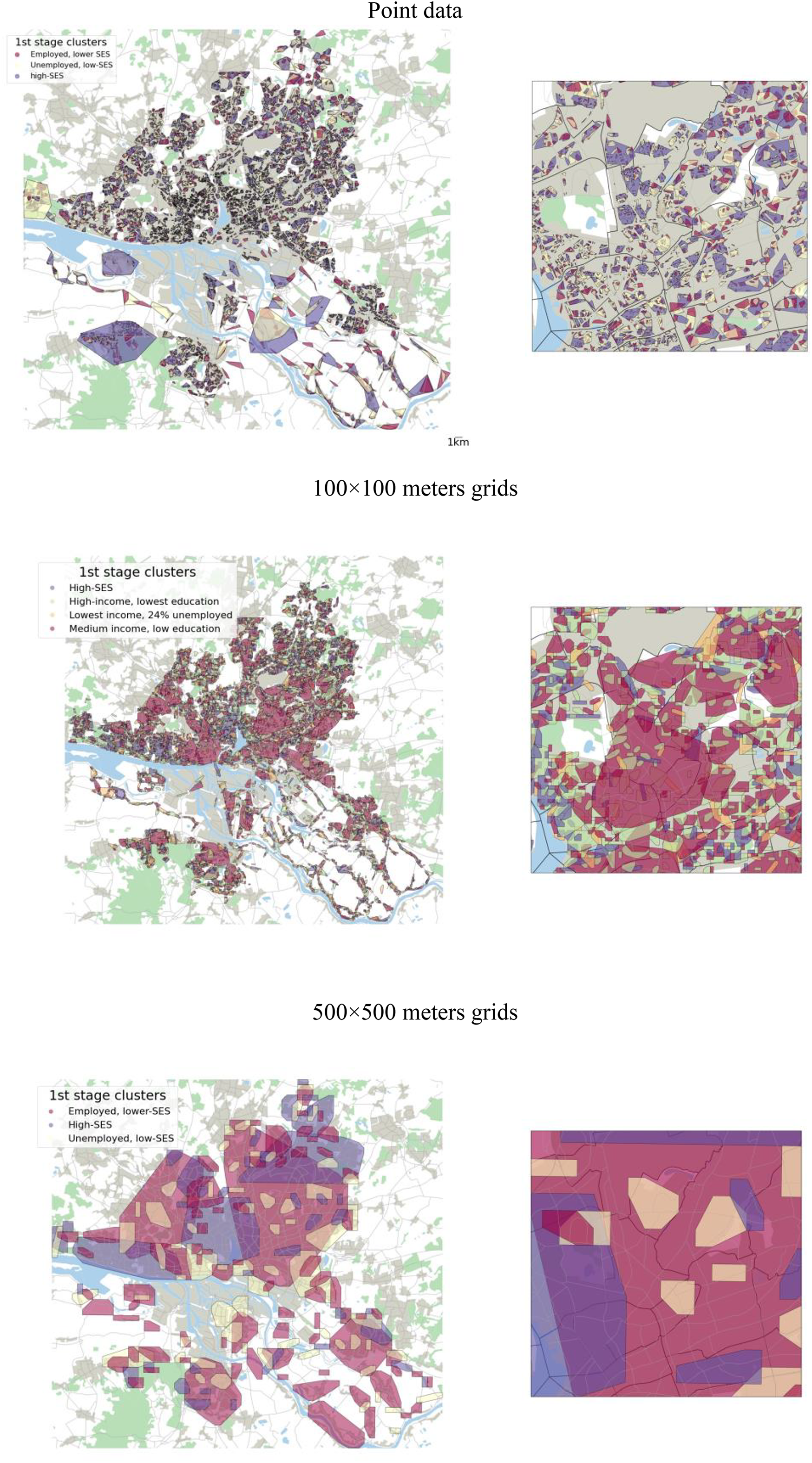
Maps visualizing the results of the two-staged clustering approach, example Hamburg. Notes: The point data maps use min_cluster_size = 25 and the grid data maps min_cluster_size = 2. Each polygon is one organic neighborhood. The background map also displays water, forests, settlements; and larger roads. The maps on the right also display administrative city district borders.

Looking at the two maps in panel A, two main attributes of the organic neighborhoods stand out. First, the neighborhoods vary in shape. While some neighborhoods resemble circles or squares, as in the western part of the city, others are more elongated, especially in the southeastern part of the city. When looking at the smaller-scaled map, these different shapes of neighborhoods sometimes follow administrative borders and reflect differences in local infrastructure, such as water bodies, or differences in the settlement structure of residential groups. The better fit to the local infrastructure becomes even clearer when comparing the organic neighborhoods with grid cells as neighborhood measure (see Figure A.9 in Appendix A.5 in the online supplement). Second, the neighborhoods vary in size. Some neighborhoods are relatively large, while others—especially those near the city center—are very small. Here, the density-based algorithm performs in accordance with theory: in more anonymous and dense city centers, social neighborhoods are expected to be smaller than in suburban neighborhoods, which have lower densities. For Hamburg, I also observe that high-SES neighborhoods tend to be larger (0.87km², roughly equals 124 soccer fields) than the lower SES neighborhoods (unemployed: 0.40km², employed: 0.11km², roughly equals 15 soccer fields). These area sizes match previous research on egohoods which identifies 300 m radius egohoods (0.283km²) as most relevant proxy for neighborhood segregation in many European cities (Marcinczak et al. 2023).

Appendix A.4 in the online supplement examines the average neighborhood characteristics for all cities and min_cluster_size=25 in greater detail and provides additional maps for other cities than Hamburg. The average inner-city neighborhood consists of 56 individuals ¹¹ and has an average area per resident of 607m². ¹² Mirroring the single-city evidence for Hamburg, high-SES neighborhoods are larger than low-SES neighborhoods, which is even more apparent when looking at the area per resident. In addition, high-SES neighborhoods overlap with a greater number of other neighborhoods than low-SES neighborhoods.

Appendix A.3 in the online supplement gives more information on how the mean neighborhood characteristics change when varying the hyperparameters min_cluster_size and min_samples. In summary, increasing values for min_cluster_size proportionally increase the neighborhood size in terms of area and population. Increasing values for min_samples slightly improves computational intensity, but does not substantially change the number of identified neighborhoods or their sizes. Higher values of min_cluster_size and lower values of min_samples decrease the noise ratio, that is, the number of observations that are not assigned to any neighborhood. Taken together, researchers who would like to use the algorithm to measure social processes in neighborhoods based on knowing each other by face should choose smaller values of min_cluster_size. Researchers interested in segregation processes on a similar level like tracts or blocks should choose larger values of min_cluster_size. To select min_samples, researchers can optimize the ratio between computational intensity and white noise.

To investigate segregation processes, researchers can also use coarser input data such as grid cells instead of point data. Panels B and C in Figure 1 display four maps using such grids as input data for Hamburg. As expected, the area and the number of residents of an average neighborhood are substantially larger. An average neighborhood comprises six 100 × 100 resp. nine 500 × 500 m grids and 131 resp. 3,584 residents. Hence, the organic neighborhoods based on 500 × 500 m grids have a similar number of residents as smaller Census tracts. ¹³ Using coarser data such as grids shows that researchers can also employ the algorithm to spatially coarser input data to obtain larger neighborhoods. As the paper focuses on capturing similar norms, routines, and behavior being more likely among smaller groups, the main analyses will continue with point data but Appendix A.5 in the online supplement provides full analyses using grids.

Application: Organic Neighborhoods and Crime

To provide a first intuition of why organic neighborhoods with time-dynamic boundaries improve our sociological understanding of neighborhood effects, the second part of the article provides an application that examines city crime rates following the notion of social disorganization theory (Sampson and Groves 1989; Shaw and McKay 1942). Explaining differences in crime between neighborhoods is one of the earliest topics in neighborhood research investigated by many excellent studies (e.g., Hipp 2007; Legewie and Schaeffer 2016; Mayer and Jencks 1989; Sampson and Groves 1989). Therefore, crime is an obvious topic to test whether we gain additional knowledge about neighborhoods by exploiting the unique attributes of the organic neighborhoods proposed in this article. While the high granularity of the data would also allow neighborhood-level analyses, the application provides a city-, that is, macro-level analysis. Such macro-level analyses are especially useful when investigating the add-on of organic neighborhoods in the relationship between aggregate population characteristics (e.g., average income or unemployment of a city) and changes in the neighborhood composition (Rey et al. 2011: 58).

Social Disorganization Theory

First introduced by Shaw and McKay (1942), social disorganization theory became one of the most important theories to explain the spatial dimension of criminal behavior (Hipp 2007; Legewie 2018; Sampson and Groves 1989). Social disorganization theory defines three structural characteristics of a community that impede realizing a joint set of values and maintaining social controls (Sampson and Groves 1989; Kornhauser 1978): low economic status, high (ethnic) heterogeneity, and high residential mobility. According to social disorganization theory, a community with these characteristics cannot build formal and informal networks to solve common problems (Sampson and Groves 1989). This inability ultimately leads to a disruption of the community's social organization, which manifests itself in higher crime rates overall.

The structural characteristic socioeconomic status refers to a neighborhood's endowment. Neighborhoods with a high proportion of poor people lack money and resources that help maintain social control and combat rising criminal activity (Hipp 2007). Conversely, wealthy neighborhoods with more resources should have less crime. Refining the neighborhood endowment hypothesis, Cohen and Felsen (1979) emphasized the spatial embeddedness of the offender. While high-income neighborhoods should generally show less crime, proximity to low-income neighborhoods can make high-income neighborhoods attractive targets that ultimately show higher crime rates than expected (Hipp 2007).

Originally based on ethnicity, the second structural characteristic is neighborhood heterogeneity. Although Shaw and McKay (1942) mentioned ethnic heterogeneity as the main dimension of neighborhood heterogeneity, the mechanism also works for other dimensions, which might be important in European countries. The basic mechanism is that as heterogeneity increases, the frequency of interaction is likely to decrease (Melamed et al. 2020) and consensus on shared norms is more difficult to achieve, ultimately leading to higher crime (Hipp 2007; Sampson and Groves 1989). In addition to the mere existence of heterogeneous groups, the relative size of groups can also affect neighborhood crime rates. Large, homogeneous groups have more power, which allows them to set and shape local norms more effectively than relatively smaller groups (Galster 2014). Consequently, a fragmented area with many diverse and small neighborhoods should have more crime than a similarly sized area populated by one large homogeneous group.

Focusing on contested boundaries, Legewie and Schaeffer (2016) emphasize a subdimension of neighborhood heterogeneity. The authors use an edge detection algorithm (Legewie 2018) to distinguish between tracts with fuzzy and well-defined boundaries. At fuzzy boundaries, heterogeneous groups “fight” for the local superiority status. Although social disorganization theory predicts that heterogeneity generally increases neighborhood conflict, Legewie and Schaeffer (2016) find that neighborhood complaints peak in neighborhoods with fuzzy boundaries, that is, between heterogeneous neighborhoods without clear boundaries.

The third and final structural characteristic is residential mobility, more broadly defined as the (in)stability of neighborhoods. Neighborhoods with high residential turnover have difficulty developing stable community networks and shared neighborhood identities, the absence of which increases crime (Sampson and Groves 1989). In terms of neighborhood boundaries, high-turnover neighborhoods may also exhibit spatially shifting boundaries over time. While Legewie and Schaeffer (2016) have shown for two separate years that neighborhood conflict increases at contested boundaries, these social processes also likely have a temporal dimension. If temporal boundary shifts mark fuzzy boundaries, then crime should be greater in heterogeneous areas with shifting boundaries.

Descriptions on the Development Over Time

Before investigating the relationship between neighborhood characteristics and city crime in a regression framework, I use descriptive and small-scale maps on the development of organic neighborhoods to exemplify the advantages of the two-staged approach and to set up first hypotheses on how those changes may affect city crime rates according to social disorganization theory.

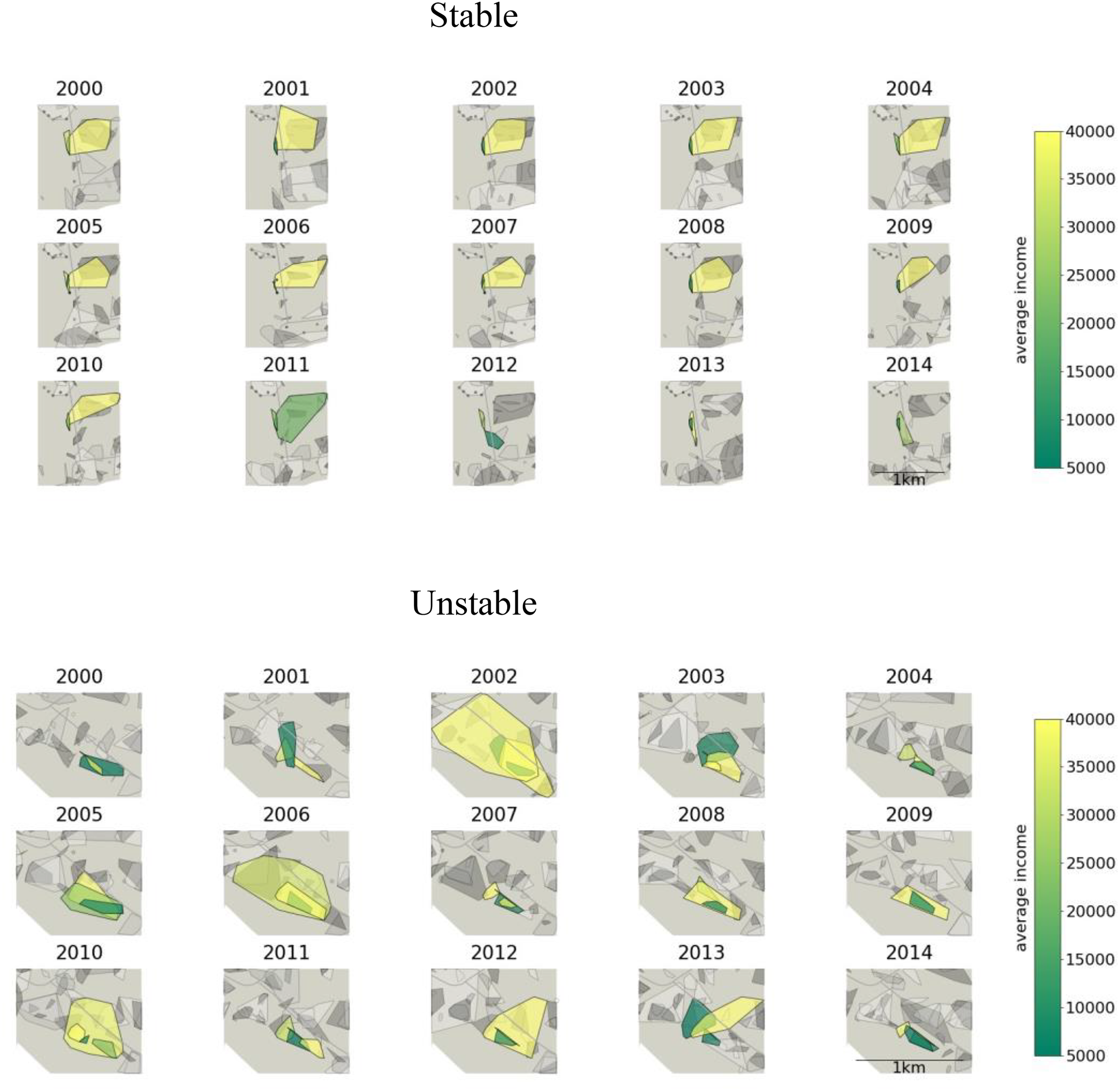
Illustrating the potential of tracing neighborhood development, Table 1 zooms in on two areas of Hamburg over 15 years and compares how the organic neighborhoods in these two areas evolve differently over time. In both areas, which span about 1 km in latitude, all existing neighborhoods and their evolution over time are shown. For sparsity and clarity, each set of maps highlights only one set of overlapping neighborhoods. Other nonoverlapping neighborhoods in the same area are grayed out. The color of the neighborhood represents the median income of its residents, with green indicating a lower median income and yellow indicating a higher median income. Similarly, lighter shades of gray indicate a higher median income for the neighborhoods in the background. Gray lines represent larger roads. The top panel shows an example of a stable area, while the bottom panel shows an example of a more unstable area.

Table 1.

Examples for a Stable and an Unstable Neighborhood.

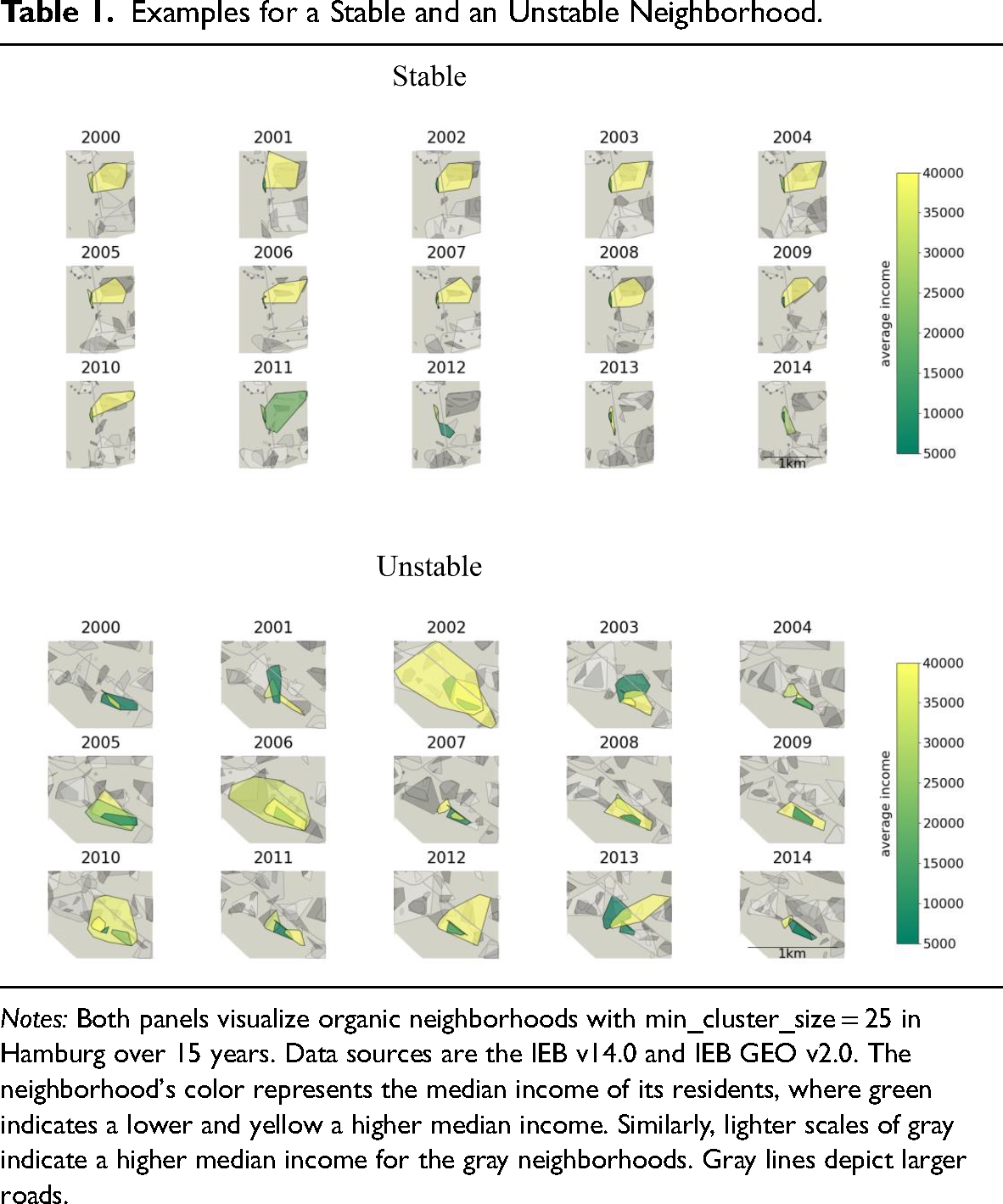
Notes: Both panels visualize organic neighborhoods with min_cluster_size = 25 in Hamburg over 15 years. Data sources are the IEB v14.0 and IEB GEO v2.0. The neighborhood's color represents the median income of its residents, where green indicates a lower and yellow a higher median income. Similarly, lighter scales of gray indicate a higher median income for the gray neighborhoods. Gray lines depict larger roads.

The area labeled stable represents two highlighted neighborhoods from 2000 to 2014. The first stable and low-income neighborhood (green) is really small, probably only a few houses with an average of 64 residents, but remained in this area throughout the entire observation period. Another stable but high-income neighborhood (yellow) with a more cubic shape is present in the area until 2010. Although the higher-income neighborhood shows a similar number of residents (69 on average), it has a larger area than the lower-income neighborhood. The boundaries of the high-income neighborhood shift somewhat over time, but the neighborhood size remains nearly constant for 11 years. In 2011, the former higher-income neighborhood transformed into a low-income neighborhood and then fragmented into smaller neighborhoods until the end of the observation period.

Although the area labeled unstable includes also some stable neighborhoods, such as the longish low-income neighborhood in the lower right part of the maps, the majority of the neighborhoods show high volatility over time. Several neighborhoods of different income levels emerge or disappear, grow, or shrink over time.

This instability may be due either to high levels of residential mobility or to changes in the characteristics of the residents already living in the area. Since similarity in income, education, and employment status labels residents of the same neighborhood, becoming unemployed can be such a change in characteristics. To investigate the underlying dynamic in greater detail, I check the residential mobility of the areas’ residents and the development of their aggregate characteristics. The results show that moving individuals mainly drive the changes in both areas while the aggregate statistics remain relatively constant for both areas over time (see Figures A.12 and A.13 in the online supplement).

Several differences between the two areas allow hypotheses about differences in crime when examining the three structural characteristics endowment, heterogeneity, and mobility, all of which are considered to be conducive to social disorganization. Comparing the average endowments of the areas, the two areas do not differ much from each other. Until 2011, the colored neighborhoods in the stable area show an average income of 35,000 Euros and the neighborhoods in the unstable area 36,000 Euros. The median income in the unstable area, at 33,000 Euros, is not much lower than the average, while the median income in the stable area (28,500 Euros) is much lower, indicating that high-income neighborhoods drive the average. When hypothesizing about the prevalence of crime, the endowments of the areas do not allow for a clear prediction. Both areas have similar endowments until 2011. When considering the development over time, however, social disorganization theory would predict a more positive trend in the crime activities in the stable area, especially after 2011 when the average income decreased.

Concerning neighborhood heterogeneity, the predictions for crime differences are clearer. The set of overlapping neighborhoods in the stable area contains 51 neighborhood × year observations with an average of 64 residents, while the set of neighborhoods in the unstable area contains 65 observations with an average of 109 residents. Although the set of neighborhoods in the unstable area contains more neighborhoods and residents, the average neighborhood in the unstable area is 0.6km² smaller than the average neighborhood in the stable area. In terms of crime, the higher density and larger number of neighborhoods of the unstable area would predict higher crime rates in the unstable area.

While the boundaries of the stable neighborhoods barely change, entire neighborhoods in the unstable area appear or disappear, grow, or shrink over time. Because the shifting boundaries reflect either residential mobility or changes in the characteristics of those who remain, the unstable area experiences more turnover than the stable area, leading to predictions of higher crime in the unstable area.

Data, Variables, and Methods

To test the specified hypotheses, I merge the organic neighborhoods with open-source data from the Police Crime Statistics (PKS), which the German Federal Criminal Police Office provides annually at the city level. In contrast to other countries, lower-level registry data on crimes, such as those at the district level, are not publicly available for research purposes in Germany. The city-level data contain summary statistics on the total number of reported crimes ¹⁴ and reported crime cases by type of crime for all German cities with more than 100,000 inhabitants (N = 76) since 2013.

The dependent variable is crime cases per 100,000 inhabitants. By dividing the number of cases by the number of a city's inhabitants, I create a measure that is more comparable for cities of different sizes. In the sample, the mean number of total crime cases is close to 10,000 crime cases per 100,0000 inhabitants, with a minimum of 4,650 (Fürth in 2017) and a maximum of 17,000 cases (Trier in 2016). While the distribution is not perfectly normal, the city-level measure of total crime cases is less skewed to zero than typical crime measures at lower spatial scales (see Figure A.14 in the online supplement).

The explanatory variables for the regressions are aggregate information on the city's neighborhoods organized in three sets of characteristics considering the neighborhoods’ SES, heterogeneity, and stability.

In analyzing the average endowment of a city's neighborhoods, I consider the level of resources, their spatial expansion, and potential spillover effects to other parts of the city. A larger number of high-SES neighborhoods, that is, neighborhoods with higher income and education levels, represents a larger number of well-resourced communities that should be more effective at maintaining social control and combating rising criminal activity. While quantifying the linear relationship between an additional high-SES neighborhood and city crime provides an initial measure of city endowment, the relative size of high-SES neighborhoods also affects city crime rates. If a given number of high-SES neighborhoods occupy a large fraction of a city's land area, crime rates should be lower than in a city where the same number of neighborhoods occupies less space. To capture this mechanism, I include the area share of high-SES neighborhoods in the total city area as an explanatory variable. The third and final dimension of neighborhood endowment accounts for spillover effects from high-SES neighborhoods. In terms of crime, such spillovers can be positive, such as high-SES neighborhoods improving local infrastructure or setting positive role-model norms, or negative, such as being an attractive target for criminals. As organic neighborhoods can overlap and intersect with each other, I include the fraction of high-SES neighborhoods that share land with other neighborhoods as a measure for spillover effects. Higher values represent open SES neighborhoods with many overlaps with other neighborhoods, while values close to zero represent closed neighborhoods with no overlaps with other neighborhoods.

To measure neighborhood heterogeneity, I use the total number of organic neighborhoods, the number of different social groups present in a city, the average neighborhood area per resident, and the income gap between high and low-SES neighborhoods. A small total number of neighborhoods for a given city size indicates that only a few social groups share the same space, which would imply less social tension and lower crime rates. A related measure is the number of first-stage clustering groups that are prevalent in the city. Being the result of the algorithm's first stage, the number of K-Means groups indicates how many social groups are present in the city. Again, more social groups within a city indicate more heterogeneity, which would imply higher crime rates. Another dimension of heterogeneity is the space each group occupies. Denser neighborhoods, such as those with large apartment buildings, tend to be more anonymous than less dense suburbs. The average area per resident captures differences in residential density across the city. As a final dimension, I include the city's gap between the median income of high and low-SES neighborhoods. The larger the gap in a city, the greater the economic distance between different SES groups, making interaction and consensus on shared norms between groups more difficult.

To measure the temporal stability of neighborhoods each year, I count how many years in a row a given neighborhood exists in exactly this form, that is, has temporally constant neighborhood boundaries. I define a neighborhood as temporally stable only if its boundaries do not change at all. Therefore, I consider marginal changes, such as an additional house, as changing boundaries, which makes my definition relatively strict. After calculating the cumulative sum of a neighborhood's stable years, I reset the number each time the neighborhood changes in size or shape. Finally, I aggregate the cumulative sums of all neighborhoods to a city average for each year. Higher values of this average neighborhood age variable represent cities with more temporally stable neighborhoods. However, a lack of stability can be either due to a city's higher fragmentation into lower-SES neighborhoods, which should positively affect crime rates, or due to gentrification, that is, the expansion of high-SES neighborhoods throughout the city, which should negatively affect crime rates. To differentiate whether low levels of stability are due to a spatial expansion of high-SES neighborhoods across the city area, I additionally include an interaction between the neighborhoods’ stability and the relative area share of high-SES neighborhoods on the total city area.

To examine the relationship between crime rates and the explanatory variables, I eschew negative binomial regressions in favor of standard OLS regressions. Because many crime measures rely on over-dispersed count data, most papers on crime use negative binomial regressions that reweight observations in the tails of the distribution (Ver Hoef and Boveng 2007). However, when considering crimes per 100,000 inhabitants, my city-level crime measure does not follow this typical pattern. Therefore, I opt for standard OLS because of the higher robustness and less strict assumptions. To check the extent to which the OLS results reflect constant differences between cities, I additionally use first-difference (FD) regressions in the online supplement to identify the short-term effects of neighborhood change on city crime rates. FD regressions regress the difference between period t and t−1 of the dependent variable on the differences between the explanatory variables. As a consequence, FD models estimate short-term effects of changes in the explanatory variables net of level effects or constant unobserved heterogeneity. More explicitly, FD models provide a less biased estimate for dynamic effects, while preventing analyses on level and constant endowment effects. Altogether, I set up the following regression equation to analyze the relationship between the three structural neighborhood factors and city crime rates: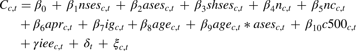

$$\begin{array}{rl}{C}_{c,t}& ={\beta }_0+{\beta }_{1}nse{s}_{c,t}+{\beta }_{2}ase{s}_{c,t}+{\beta }_{3}shse{s}_{c,t}+{\beta }_4{n}_{c,t}+{\beta }_{5}n{c}_{c,t}\\ & +{\beta }_{6}ap{r}_{c,t}+{\beta }_{7}i{g}_{c,t}+{\beta }_{8}ag{e}_{c,t}+{\beta }_{9}ag{e}_{c,t}*ase{s}_{c,t}+{\beta }_{10}c{500}_{c,t}\\ & +\gamma ie{e}_{c,t}+{\delta }_t+{\xi }_{c,t}\end{array}$$

where C_c,t denotes the crime rates per 100,000 inhabitants in city c in year t. The variables nses_c,t, ases_c,t, and shses_c,t capture the aggregated neighborhoods’ endowment, while n_c,t, nc_c,t, apr_c,t, and ig_c,t measure the aggregated neighborhoods’ heterogeneity in SES on city level. age_c,t denotes the mean neighborhood age and measures the aggregated neighborhood stability.

I include three kinds of control variables to disentangle the aggregated neighborhood effects from population size, general city-level effects of the SES input data, or time trends. The crime prevalence in huge cities like the capital city Berlin often follows different patterns than in smaller metropolises. To capture this heterogeneity, I include c500 _c,t indicating whether the city has more than 500,000 inhabitants. Moreover, I control for the general level of income, education, and employment with the matrix iee_c,t. δ_t captures year fixed effects and ξ_i,t displays the idiosyncratic error term. To make the effect sizes comparable, I standardize all explanatory variables. Supplemental Table A.3 gives an overview of the sample means for all explanatory and control variables.

Regression Results

Figure 2 presents the results for city-level crime cases per 100,000 inhabitants in six OLS regressions, each running the same model but using incrementally increasing values of the hyperparameter min_cluster_size. The estimates with min_cluster_size = 25 report the best fit with the lowest Akaike Information Criterion (AIC, see Table A.4 in the online supplement for the full regression table).

Figure 2.

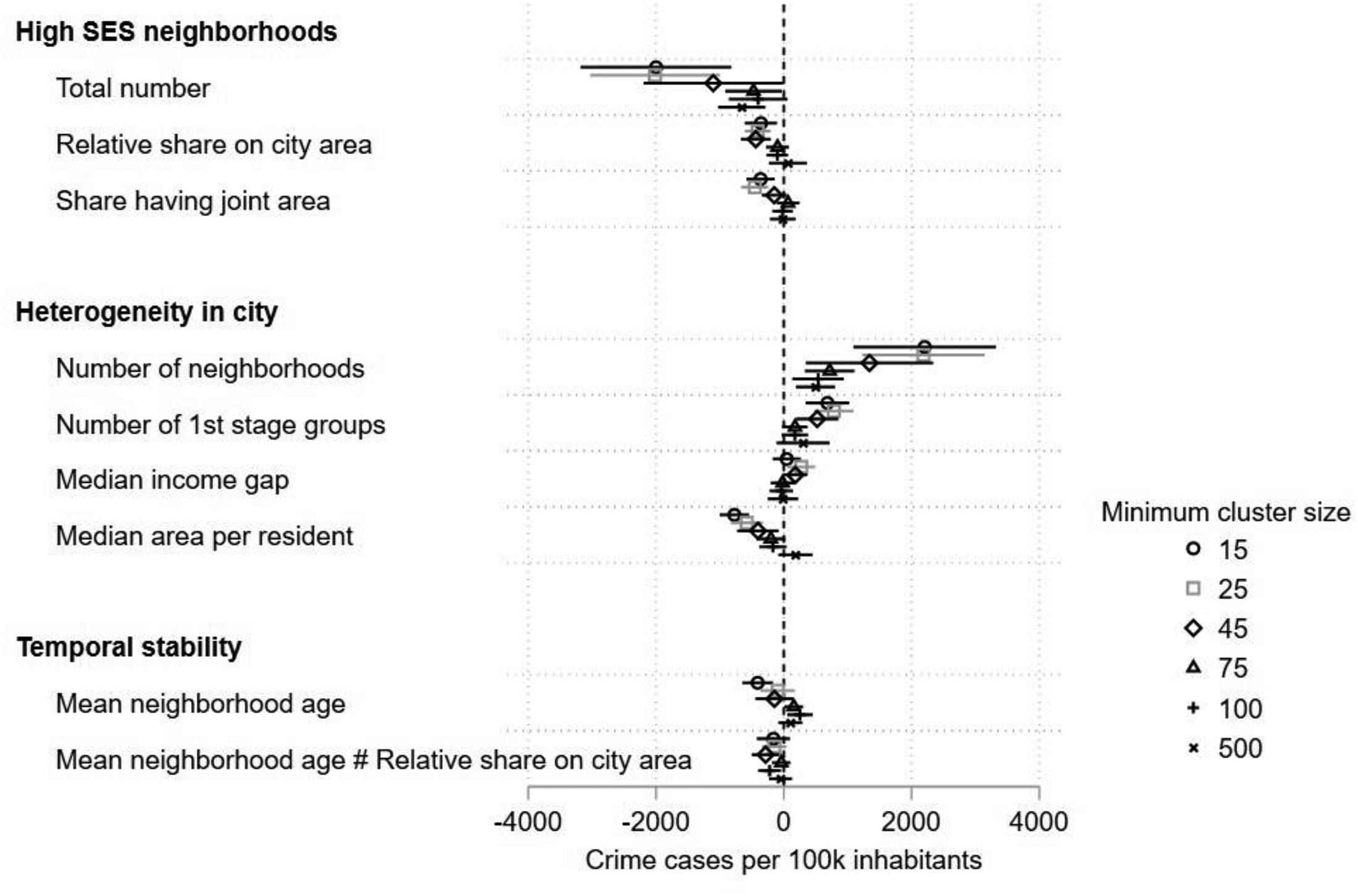
Regression results on the association between neighborhood characteristics and city crime.

For the variables measuring neighborhood endowment, all three measures point to a significant and negative relationship with the city crime rates. In all min_cluster_size specifications, a higher number of high-SES neighborhoods, a larger area share of high-SES neighborhoods in the total city area, and a higher share of high-SES neighborhoods that share space with other neighborhoods are negatively correlated with crime cases per 100,000 inhabitants. Comparing the coefficient sizes, the number of high-SES neighborhoods shows the largest coefficients. Consequently, not only the level but also the spatial distribution of resources across the city matters when analyzing crime.

In terms of neighborhood heterogeneity, a higher degree of inner-city neighborhood fragmentation is positively associated with city crime rates. The positive and significant coefficients of the number of neighborhoods and the number of first-stage clusters signal a positive relationship between increasing local diversity in SES and local crime rates. In measuring the diversity of residents in an area or a city, these results confirm previous studies on the effect of segregation and social disorganization. The aggregate measure of the socioeconomic distance between high- and low-SES neighborhoods, that is, the income gap between the city's high- and low-SES neighborhoods, does not show a significant relationship with city crime rates. Confirming the hypothesis that a lack of (personal) space favors crime, the coefficient of median area per resident indicates that cities with denser neighborhoods face more crime even when other factors such as city size are held constant. All these findings show similar trends for different min_cluster size specifications but the coefficients decrease in size for larger min_cluster_size values. Similar to the endowment dimension, the standardized total number of neighborhoods variable shows the largest coefficients.

Measuring the neighborhoods’ stability, the final explanatory variable mean neighborhood age provides less clear results across the six different hyperparameter specifications. Social disorganization theory hypothesizes a negative relationship between stability and crime. However, only the smaller min_cluster_size specifications show a negative sign and only one of those is statistically significant. The interaction terms examine whether the effects of neighborhood (in)stability are associated with a higher share of high-SES neighborhoods in the total city area. All interaction terms have a negative sign, indicating that the negative effect of neighborhood stability is most prominent in cities with a high share of high-SES neighborhoods. Hence, the results point more toward gentrification being the underlying mechanism between neighborhood stability and lower crime rates rather than a higher fragmentation into lower SES neighborhoods.

When investigating the general role of min_cluster_size, the results point toward smaller organic neighborhoods mirroring the social processes and crime dynamics better than larger values. For nearly all explanatory variables, the model estimates the largest coefficients for the smallest values of min_cluster_size. These findings align with previous findings using egohoods (Hipp and Boessen 2013) and support psychological theories about increased contact frequency in smaller groups.

Using 500 × 500 meters grid cells as input data, Figure A.11 in online supplement A.5 reports the results for the same analyses but for larger organic neighborhoods mirroring the residential population of smaller Census tracts. The basic pattern is the same as using point data as input, but using grids as input provides substantially lower and mostly insignificant point estimates with larger confidence intervals. Based on these findings and the larger confidence intervals, I consider more fine-grained data as a more appropriate input for empirically constructing organic neighborhoods and for measuring neighborhood effects on city crime in the German context.

To investigate whether the findings are mainly due to level differences between years and cities or also hold in a more dynamic setting, Table A.5 in the online supplement reruns equation (6.3) with an FD setup. In summary, only neighborhood stability shows a significant and negative effect on city crime rates in German metropolises. Hence, short-term changes in the number of (high-SES) neighborhoods or changes in the relative proportion of SES groups do not show a significant correlation with short-term changes in the city's crime rates. In terms of neighborhood stability, if the mean neighborhood age increases by 1 year, meaning that no neighborhoods in the city change their size and shape from one year to another, the crime cases per 100,000 inhabitants decrease by 51 (min_cluster_size = 500) to 2900 (min_cluster_size = 15) cases per 100,000 inhabitants. While being a relatively rough measure on the city level, the estimates still point toward being a meaningful empirical starting point for testing the theoretical concept of neighborhood stability for future research with data on a lower spatial level.

Discussion

This article introduced a new data-driven approach to construct dynamic organic neighborhoods of varying size, shape, and population density. While previous network approaches based on interaction data substantially improved the measurement of neighborhoods, limited data access, the high computational intensity, and the subordinate role of spatial distance in the algorithms still impede a realistic measure of neighborhood and neighborhood evolution. Constructed in a two-staged design, the newly proposed approach first identifies similar individuals in a city and then defines spatially proximate similar individuals as neighbors. The resulting organic neighborhoods not only capture the social reality of residents better but also treat neighborhoods as nonconstant entities, whose changing sizes and forms signal meaningful local processes. Unlike previous approaches, the two-staged unsupervised learning approach allows to tailor the size of the neighborhoods to the researcher's research purposes in altering the hyperparameter min_cluster_size while showing a high computational efficiency.

A proof-of-concept application in the second part of the article has not only shown how researchers can use organic neighborhoods to analyze the relationship between neighborhood disorganization and city crime but also why researchers must consider organic neighborhoods as an aspect of individuals’ reality. In decomposing the neighborhood characteristics in endowment, heterogeneity, and stability, I can show that especially the number of organic neighborhoods and the number of high-SES neighborhoods correlate with city crime rates. A higher total number of neighborhoods in a city indicates local fragmentation, that is, increasing heterogeneity, whereas a higher number of high-SES neighborhoods in a city indicates increasing levels of local endowment. From a dynamic perspective, the mean neighborhood stability shows the highest impact on city crime rates. As previous quantitative studies mainly focused on level differences between or compositional changes within neighborhoods, this study confirms that organic neighborhoods are “agentic player[s]” (Shedd 2015: 8) whose changes may explain differences in criminal activity between cities and over time.

In providing a data-efficient and transparent approach to construct social neighborhoods, this study points toward several open strands for future research. While the two-staged clustering algorithm improves the measurement of neighborhoods compared to previous aggregation approaches, an important task for future research is to combine the proposed algorithm with interaction data. Studies like Hipp et al. (2012) or Levy et al. (2020) have already shown that interaction is an important dimension in explaining neighborhood and segregation effects. By directly using interaction data as input for the two-staged clustering algorithm, neighborhood researchers would be able to combine the advantages of relying on interaction data and using a neighborhood approach that directly considers the spatial dimension of neighborhoods. In doing so, neighborhood researchers do not have to rely on the assumption that similarity fosters interaction anymore but can directly test how social composition predicts interaction and vice versa. In the analysis of crime, a combination of both approaches could also enable testing how membership in and endowment of other social networks affect the social organization of residential neighborhoods.

This article analyzed how neighborhood features correlate with crime at the macro-level of cities. Due to the paper's methodological focus, the proof-of-concept application remains necessarily coarse. Future research should not only analyze the relationship and the local dynamics on a lower spatial level in greater detail to exploit the full potential of the concept of organic neighborhoods but also investigate the organizational and informal factors explaining why certain neighborhoods remain stable and others do not. A fruitful avenue would be to consider mechanisms of formal and informal organization using, for example, web-scraped data on schools, churches, or cultural amenities.

Going beyond neighborhood crime, the two-staged approach could also be employed to cluster individuals, firms, or even regions more flexibly and transparently than previous methods had done. In using data on individuals’ ethnicity, future research can use the algorithm to investigate temporal and spatial processes of ethnic enclaves or white flight (Crowder 2000; Kye and Halpern-Manners 2022). Organic neighborhoods can also improve the description of segregation patterns within cities, for which grid-cell analyses already point towards substantial differences across German cities (Ostermann et al. 2022; Ostermann and Wolf 2023; Rüttenauer 2022). In using firm data, the algorithm can model the emergence and development of tech hubs and excellence clusters. Ultimately, in employing data on larger geographical units such as grids, tracts, and counties for the first stage, the algorithm provides spatial units useful for controlling for or directly analyzing contextual effects.

Taken together, this article contributes not only to the literature on improving the measurement of neighborhoods but also stresses the potential of big data and computational social science for sociological research on contextual effects. Dedicated knowledge about the advantages and disadvantages of certain algorithms offers plentiful opportunities to improve the quantitative measurement of (perceived) social realities and, ultimately, sociological research.

Supplemental Material

sj-pdf-1-smr-10.1177_00491241261420810 - Supplemental material for Beyond Proximity: Investigating Crime With Organic Neighborhoods and a Two-Stage Unsupervised Learning Approach

Supplemental material, sj-pdf-1-smr-10.1177_00491241261420810 for Beyond Proximity: Investigating Crime With Organic Neighborhoods and a Two-Stage Unsupervised Learning Approach by Kerstin Ostermann in Sociological Methods & Research