The Effects of Omitting Components in a Multilevel Model With Social Network Effects

Abstract

Multilevel models are often used to account for the hierarchical structure of social data and the inherent dependencies to produce estimates of regression coefficients, variance components associated with each level, and accurate standard errors. Social network analysis is another important approach to analysing complex data that incoproate the social relationships between a number of individuals. Extended linear regression models, such as network autoregressive models, have been proposed that include the social network information to account for the dependencies between persons. In this article, we propose three types of models that account for both the multilevel structure and the social network structure together, leading to network autoregressive multilevel models. We investigate theoretically and empirically, using simulated data and a data set from the Dutch Social Behavior study, the effect of omitting the levels and the social network on the estimates of the regression coefficients, variance components, network autocorrelation parameter, and standard errors.

Introduction

In the quantitative analysis of social data it is increasingly recognized that people are not independent of each other and any analysis should account for their social contexts and connections. Multilevel analysis is carried out routinely to take into account group dependencies arising from people being members of groups such as households, geographical groups such as neighborhoods and organizational groups such as hospitals or schools.

Another source of dependencies for individuals, which may cross the other groups to which they belong, is their social network. While social network analysis (SNA) has recently received much attention in the social sciences, SNA researchers often ignore other aspects of the multilevel population structure. Moreover, most multilevel modelers consider group dependencies (e.g., students in schools), but tend to ignore social network dependencies in their analysis (e.g., students’ friendship networks). In this article, we develop a new class of models called network autoregressive multilevel models (NAMLMs), which include both social network effects and multilevel effects that account for group dependencies when undertaking a regression analysis of a response variable on a set of explanatory variables. It is common to include only some of these effects in an analysis, either because they are not considered or because of data limitations. Our aim is to assess the effects of omitting the social network or group dependencies, both theoretical and empirically.

If groups, such as households, local areas, or networks, are present in a population, two people within the same group tend to be more similar than two people, each from a different group. Multilevel models (MLMs) allow for modeling this similarity. These models often focus on hierarchical groups, although through cross-classified models non-hierachical groupings can be included (Goldstein 2011). MLMs are usually specified that assume the group effect is the same for all individuals in a particular group, although more complex models can be used. An example of three inter-connected groupings of individuals is people within households, neighborhoods and networks. Another example is students within classes and schools and friendship networks.

Failure to account for dependencies in a population usually leads to incorrect estimation of standard errors (SEs), leading to incorrect inferences (Berkhof and Kampen 2004; Moerbeek 2004). In some circumstances, such as in non-linear models, it may also lead to bias in the estimates of regression coefficients. Non-independence of observations was initially seen as a nuisance by statisticians, who developed methods to account for the structure of the data, such as complex survey analysis methods, see Chambers and Skinner (2003). However, the dependencies between people are often of direct substantive interest. MLMs and network autoregressive models (NAMs) provide information about these dependencies through the estimates of the parameters in these models that reflect the correlations between people, these being the variance of the group-level random effects and the associated intra-group correlations that they explain in an MLM, and the autocorrelation parameter in a network model.

In Section “Models for Multilevel Data and Social Networks,” we describe regression models that include several levels, such as households and neighborhoods or classes and schools. In Section “Models for Social Network Dependencies,” we consider popular regression models that account for dependencies induced by a social network. In Section “Extended Models That Include Social Network and Group Dependencies: Network Autoregressive Multilevel Models,” we propose three regression models that take into account the levels and a social network, and outline maximum likelihood estimation. In Section “Theoretical Impact of Omitting Some Part of the Population Structure in the Analysis,” we consider theoretically the likely impact of omitting some part of the population structure, such as levels or a network, in the analysis. A simulation study is conducted in Section “Simulation Study.” Then in Section “Example With School Data,” the models are applied to the Dutch Social Behavior Study modeling delinquent behavior of school students. This article finishes with a summary and conclusions.

Models for Multilevel Data and Social Networks

Households and Neighborhoods

A key feature of social structure is the household. Sample designs often involve the household. It is common to select one person, or all people per selected household, although other options are available (Clark and Steel 2002). Analysis of data from surveys in which all people or more than one person is selected from a household may ignore the household, which will lead to incorrect variance estimates. In some cases, both individual and household-level estimates or effects may be of interest. MLMs have also been applied in a limited way to consider the household level for phenomena such as voting behavior (Johnston et al. 2005).

Sometimes the household is ignored in analysis because a household identifier is not available, or because one person per selected household has been sampled; in this case, the household and person-level effects cannot be separated in the analysis.

Consider individual $i$ , who has response variable $Y_i$ and a vector of $p$ explanatory variables ${\mathbf{x}}_i$ , for $i=1,\cdots ,N$ . A standard two-level linear regression model including a household random effect for individual i in household j, for $j=1,\cdots ,M_2$ , is

$$Y_i={\mathbf{x}}_i^{\mathrm{\top }}\mathit{\beta }+u_j^{(2)}+{\epsilon }_i,$$

(1)where $\mathit{\beta }$ is the vector of $p$ regression coefficients, ${\epsilon }_i\sim N(0,{\sigma }_1^2)$ and $u_j^{(2)}\sim N(0,{\sigma }_2^2)$ are the individual (level 1) and household (level 2) random effects, respectively.

Individuals can be grouped into geographical areas. Statistics are produced for geographical areas, such as local authorities, post-codes, or census output areas. Geographical areas may be used in the selection of the sample for a survey, through the use of cluster or multistage sampling. Multilevel modeling has been used for individuals grouped in areas, possibly incorporating contextual variables such as area level means of explanatory variables (Goldstein 2011), with respect to health, see, for example, Subramanian, Jones, and Duncan (2003), for unemployment, see Fieldhouse and Tranmer (2001), and other social outcomes. Standard MLMs assume constant within area correlations between individuals and no correlations across areas, although the latter assumption can be loosened.

A random effect can be added to (1) for areas, where the individual is indexed by $i$ , the household by $j$ , and the area by $k$ , for $k=1,\cdots ,M_3$ :

$$Y_i={\mathbf{x}}_i^{\mathrm{\top }}\mathit{\beta }+u_j^{(2)}+u_k^{(3)}+{\epsilon }_i,$$

(2)where $u_k^{(3)}\sim N(0,{\sigma }_3^2)$ is the area (level 3) random effect. Let $\mathbf{Y}=(Y_1,\cdots ,Y_N{)}^{\mathrm{\top }}$ and $\mathbf{X}=({\mathbf{x}}_1,\cdots ,{\mathbf{x}}_N{)}^{\mathrm{\top }}$ , then this model can be written as:

$$\mathbf{Y}=\mathbf{X}\mathit{\beta }+{\mathbf{Z}}_2{\mathbf{u}}^{(2)}+{\mathbf{Z}}_3{\mathbf{u}}^{(3)}+\mathit{\epsilon },$$

(3)where ${\mathbf{u}}^{(l)}\sim N(0,{\sigma }_l^2{\mathbf{I}}_{M_l})$ and $\mathit{\epsilon }\sim N(0,{\sigma }_1^2{\mathbf{I}}_N)$ and ${\mathbf{Z}}_2$ and ${\mathbf{Z}}_3$ are matrices with a “1” in the row corresponding to the household and area to which individual $i$ belongs, respectively. The notation ${\mathbf{I}}_N$ stands for the identity matrix of size $N\times N$ . The linear mixed model (3) implies the mean is $E(\mathbf{Y})=\mathbf{X}\mathit{\beta }$ and the covariance matrix is $\mathbf{V}=V(\mathbf{Y})={\sigma }_1^2{\mathbf{I}}_N+{\sigma }_2^2{\mathbf{Z}}_2{\mathbf{Z}}_2^{\mathrm{\top }}+{\sigma }_3^2{\mathbf{Z}}_3{\mathbf{Z}}_3^{\mathrm{\top }}$ . The intra-group correlation of two individuals in the same group at level $l$ due to the level $l$ random effect is ${\sigma }_l^2/({\sigma }_1^2+{\sigma }_2^2+{\sigma }_3^2)$ for $l=2,3$ .

Setting $\mathbf{Z}=[{\mathbf{Z}}_2,{\mathbf{Z}}_3]$ and $\mathbf{u}=(({\mathbf{u}}^{(1)}{)}^{\mathrm{\top }},({\mathbf{u}}^{(2)}{)}^{\mathrm{\top }}{)}^{\mathrm{\top }}$ , the model is:

$$\mathbf{Y}=\mathbf{X}\mathit{\beta }+\mathbf{Z}\mathbf{u}+\mathit{\epsilon },$$

(4)with $\mathbf{D}=V(\mathbf{u})=[\begin{array}{cc}{\sigma }_2^2{\mathbf{I}}_{M_2}& 0\\ 0& {\sigma }_3^2{\mathbf{I}}_{M_3}\end{array}].$ Hence the covariance matrix can be written as $V(\mathbf{Y})={\sigma }_1^2{\mathbf{I}}_N+\mathbf{Z}\mathbf{D}{\mathbf{Z}}^{\mathrm{\top }}.$

Classes and Schools

For educational data on students, the information on the classes and schools is incorporated into the MLM, as students are nested within classes and classes within schools. The MLM has students as level 1 units, classes as level 2 units, and schools as level 3 units (Berkhof and Kampen 2004). The residual errors, ${ϵ}_i\sim N(0,{\sigma }_1^2)$ , refer to students, the lowest level, the random effects, $u_j^{(2)}\sim N(0,{\sigma }_2^2)$ , to classes and the random effects, $u_k^{(3)}\sim N(0,{\sigma }_3^2)$ , to schools. The model can also be written as (2), (3), or (4).

Models for Social Network Dependencies

People can also be grouped by their social network, and there is growing interest in SNA following the publications of the books by Wasserman and Faust (1994), Carrington, Scott, and Wasserman (2005) and Scott (2012). Considerable work has been carried out to develop models for networks, such as exponential random graph (p*) models (Snijders et al. 2006). Reviews of statistical models for social networks were also given by Snijders (2011) and Amati, Lomi, and Mira (2018). The importance of social networks with respect to health is discussed by Kawachi and Berkman (2000, 2003), Haines, Beggs, and Hurlbert (2011) and Lusher, Koskinen, and Robins (2013).

Network Effects and Network Disturbance Models

Our interest is not in the modeling of the social network itself, but in accounting for the dependencies induced by the social network when modeling a response variable. We consider two models that allow for the effects of social network dependencies on a response variable and allow for covariates in the model. These are generally described as network autocorrelation models (NAMs) in the social network literature (Leenders 2002).

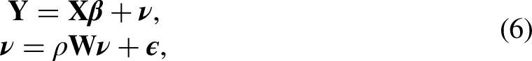
A network effects model allows for autocorrelation directly in the response variable (Leenders 2002). For a population of N individuals, one way of incorporating social network dependencies, but not other group dependencies, is via the network effects model:

$$\mathbf{Y}=\mathbf{X}\mathit{\beta }+\rho \mathbf{W}\mathbf{Y}+\mathit{ϵ},$$

(5)Here, $\mathbf{W}$ is the $N\times N$ social network connection or weight matrix for the individuals, also referred to as an adjacency matrix. If $\mathbf{W}$ is a connection matrix, an element $W_{ij}$ takes a value of 1 if individuals i and j are connected and 0 if i and j are not connected. “Connected” usually means a relationship, such as being a best friend, exists between individual $i$ and $j$ . In general, the diagonal elements, $W_{ii}$ , of $\mathbf{W}$ are set to equal 0. Sometimes $\mathbf{W}$ is not a series of connections, but is a standardized version of the binary connection matrix, or some other type of weight matrix. Leenders (2002) points out that the choice of $\mathbf{W}$ affects the results of using the model, and also makes recommendations on which $\mathbf{W}$ should be used. In this model, the response for individual i is directly related to the responses of those people connected to individual i, through the matrix $\mathbf{W}$ , and the parameter $\rho$ reflects the extent of this relationship. If $\mathbf{W}$ is a connection matrix, the relationship between the response of the focal individual and the response of each individual connected to them is assumed to be the same.

A network disturbance model allows for autocorrelation in the error term, see Leenders (2002) for a review. Here $\mathbf{W}$ can be incorporated into the model through the error term ${\nu }_i$ , as shown in the network disturbance model (6) below. The term ${ϵ}_i$ is an additional error term to account for any noise that is not reflected by the network dependencies (as ${\nu }_i$ , is assumed to do). As before, ${ϵ}_i$ is assumed to be normally distributed, with variance ${\sigma }_1^2$ , then the network disturbance model in vector form is:

$$\begin{array}{c}\mathbf{Y}=\mathbf{X}\mathit{\beta }+\mathit{\nu },\\ \mathit{\nu }=\rho \mathbf{W}\mathit{\nu }+\mathit{ϵ},\end{array}$$

(6)with $\mathit{\nu }=({\nu }_1,\cdots ,{\nu }_N{)}^{\mathrm{\top }}$ .

In the geographical literature, (5) and (6) are both examples of spatial autoregressive regression models (Lesage and Pace 2009), where the connection matrices represent geographical connections such as contiguity, or some other type of geographical link, rather than social network dependencies. In this literature, model (5) is often described as a spatially lagged dependent variable model, and model (6) as a spatial error model (Ward and Gleditsch 2008). As noted by Leenders (2002), this model can also be labeled as a spatial moving average model, see Muir (1999). Model (5) is a simultaneous autoregressive model. An alternative approach in the spatial statistics literature is a conditional autoregressive model; see Cressie (1993: section 6.3) for a discussion of these two different approaches. For this article, we generally use the terminology from the social network literature.

In the geographical literature, Ward and Gleditsch (2008:70) argue, from a social science perspective, that “if we expect to see, or are interested in, feedback, then the spatially lagged/network effects model seems most appropriate, and that the spatial error/network disturbance model is appropriate primarily when researchers believe that there is some spatial (or more generally dependence) pattern that will be reflected in the error term, but the researchers are unwilling or unable to make assumptions about the origin of the error.”

The models specified by (5) and (6) differ according to whether the network dependence is in the regression or error terms part of the model. Model (5) accounts for autocorrelation directly in the response variable, after allowing for the covariates, and would be useful when we suspect such effects exist and are substantively interested in them. In model (6), the autocorrelation is in the individual-level error terms and any apparent autocorrelation in the response variable is due to this.

The theoretical and practical similarities and differences in these two models can be clarified by considering the variance and mean structure that they imply. Set $\mathbf{A}(\rho )={\mathbf{I}}_N-\rho \mathbf{W}$ , then for both models $V(\mathbf{Y})={\sigma }_1^2{\mathbf{A}}^{-1}({\mathbf{A}}^{-1}{)}^{\mathrm{\top }}$ . The main difference is that for the network effects model (5) the mean is given by $E(\mathbf{Y})={\mathbf{A}}^{-1}\mathbf{X}\mathit{\beta }$ , whereas for the network disturbance model (6) it is $E(\mathbf{Y})=\mathbf{X}\mathit{\beta }$ . If $\rho$ is small we can approximate ${\mathbf{A}}^{-1}\approx {\mathbf{I}}_N+\rho \mathbf{W}$ , so that $E(\mathbf{Y})\approx \mathbf{X}\mathit{\beta }+\rho \mathbf{W}\mathbf{X}\mathit{\beta }$ . The matrix $\mathbf{W}\mathbf{X}=\overline{\mathbf{X}}$ can be termed a network contextual variable since the $i$ th row contains the totals (binary $\mathbf{W}$ ) or means ( $\mathbf{W}$ weighted with row-sums of 1) of the explanatory variables for the set of individuals connected to individual $i$ . The product of the parameters, $\rho \mathit{\beta }$ , can be termed the corresponding network contextual effects. Hence, our consideration in choosing these two models is whether there is reason to believe network contextual effects are present or of substantive interest. It also suggests that a simple diagnostic to check which model is appropriate is to undertake a standard regression analysis that includes $\overline{\mathbf{X}}$ in the regression part of the model. An alternative is to adopt a network disturbance model, with $\mathbf{X}$ and $\overline{\mathbf{X}}$ in the regression part of the model, although this doubles the number of regression parameters to be estimated. The role of contextual effects and considerations relevant to whether effects should be treated as random or fixed are discussed for the standard MLM, for example, by De Leeuw and Meijer (2008), and Snijders and Bosker (2012), and the arguments used are also applicable here.

Multiple Membership (MM) Models

Tranmer, Steel, and Browne (2014) and Tranmer and Lazega (2016) consider an alternative to NAMs using a particular linear mixed model, the MM model, to model the dependencies arising from the network. The MM model is:

$$Y_i={\mathbf{x}}_i^{\mathrm{\top }}\mathit{\beta }+\sum _{j\in \mathrm{group}(\mathrm{i})}{W}_{ij}{u}_j+{\epsilon }_i;i=1,\cdots ,N;\mathrm{group}(\mathrm{i})\subset 1,\cdots ,\mathrm{J}$$

(7)where $u_j\sim N(0,{\sigma }_u^2)$ is the $j$ th random effect associated with the $j$ th ego-net out of $J$ total ego-nets, and where ${\epsilon }_i\sim N(0,{\sigma }_1^2)$ are the individual error terms. The term $\mathrm{group}(\mathrm{i})$ is the set of ego-nets to which $i$ is a member. In the MM model ${\sigma }_u^2/({\sigma }_u^2+{\sigma }_1^2)$ is the analog of $\rho$ in the NAMs. The weight that is given to each individual for their ego-net membership is $W_{ij}$ . In principle the same matrix, $\mathbf{W}$ , used for the NAMs could be used for the MM model.

The MM model can be written in matrix form as:

$$\mathbf{Y}=\mathbf{X}\mathit{\beta }+\mathbf{W}\mathbf{u}+\mathit{\epsilon }.$$

(8)This model imposes a different covariance structure compared to NAMs; see Online Appendix A for details and comparisons. Our focus is on the standard NAMs and their extension to incorporate multilevel group dependencies via random effects.

Extended Models That Include Social Network and Group Dependencies: Network Autoregressive Multilevel Models

Bringing together the ideas of statistical models in social network analysis and MLMs, we can consider how the multiple dependencies associated with households, social networks, and geographical groups, for example, can be considered in the same analysis and the consequences of omitting one or more of them in an analysis. In general, we have an individual-level outcome, $Y$ , and various individual-level explanatory variables, $\mathbf{x}$ . We need to recognize that both $Y$ and $\mathbf{x}$ for person $i$ are embedded in, and influenced by, the second level (households/classes) and third level units (neighborhoods/schools), and the other people to whom the individual is connected socially. Hence we have three types of connections:

Within household/class connections.

Connections due to proximity, which may be approximated by geographical groups with a particular scale and boundary, or connections to the same school.

Connections via social networks.

We can add random effects for households and neighborhoods, or for classes and schools, in the two social network models considered inSection “Network Effects and Network Disturbance Models.” As in Section “Network Effects and Network Disturbance Models,” the social network dependence may act directly on the response variable, giving a network effects MLM. Alternatively, the network dependence may apply to the error terms, leading to a network disturbance MLM. Once random effects for the higher levels are included in the model, the network dependence may affect both the individual level and higher level random effects or just the individual level error term, leading to two versions of the network disturbance MLM. The three resulting models are described in more detail below. All these extended models combine NAMs with MLMs to produce NAMLMs. Model I: Network Effects MLM. In this model, the social network dependence acts on the response variable:

$$\mathbf{Y}=\mathbf{X}\mathit{\beta }+\rho \mathbf{W}\mathbf{Y}+\mathbf{Z}\mathbf{u}+\mathit{ϵ}.$$

(9)For this model, $E(\mathbf{Y})={\mathbf{A}}^{-1}\mathbf{X}\mathit{\beta }$ , which depends on the network through the matrix $\mathbf{A}={\mathbf{I}}_N-\rho \mathbf{W}$ . The covariance matrix is $V(\mathbf{Y})={\mathbf{A}}^{-1}({\sigma }_1^2{\mathbf{I}}_N+\mathbf{Z}\mathbf{D}{\mathbf{Z}}^{\mathrm{\top }})({\mathbf{A}}^{-1}{)}^{\mathrm{\top }}$ in which the network and random effects are multiplicative.

In the network disturbance model, the random effects may or may not be affected by the social network, leading to two types of models. Model II: Type I Network Disturbance MLM. In this model, the network dependence affects both the individual level and higher level random effects:

$$\mathbf{Y}=\mathbf{X}\mathit{\beta }+\mathit{\nu },\mathit{\nu }=\rho \mathbf{W}\mathit{\nu }+\mathbf{Z}\mathbf{u}+\mathit{ϵ}.$$

(10)For this model, $E(\mathbf{Y})=\mathbf{X}\mathit{\beta }$ , which does not depend on the network. The covariance matrix is $V(\mathbf{Y})={\mathbf{A}}^{-1}({\sigma }_1^2{\mathbf{I}}_N+\mathbf{Z}\mathbf{D}{\mathbf{Z}}^{\mathrm{\top }})({\mathbf{A}}^{-1}{)}^{\mathrm{\top }}$ in which the network and random effects are multiplicative, as they are in Model I. Model III: Type II Network Disturbance MLM. In this model, the network dependence affects only the individual level error term:

$$\mathbf{Y}=\mathbf{X}\mathit{\beta }+\mathbf{Z}\mathbf{u}+\mathit{\nu },\mathit{\nu }=\rho \mathbf{W}\mathit{\nu }+\mathit{ϵ}.$$

(11)For this model, $E(\mathbf{Y})=\mathbf{X}\mathit{\beta }$ , which does not depend on the network. The covariance matrix is $V(\mathbf{Y})={\sigma }_1^2{\mathbf{A}}^{-1}({\mathbf{A}}^{-1}{)}^{\mathrm{\top }}+\mathbf{Z}\mathbf{D}{\mathbf{Z}}^{\mathrm{\top }}$ in which the network and random effects are additive.

Maximum likelihood estimation of the parameters $\mathit{\beta }$ , $\rho$ , and ${\sigma }_l^2$ for $l=1,2,3$ for each of the three NAMLMs is outlined in the online Appendix B.

Which of these models is appropriate in a particular situation depends on theoretical and empirical considerations that are similar to those expressed in Section “Network Effects and Network Disturbance Models.” If there are substantive reasons or empirical evidence from considering diagnostics involving the network contextual variable $\overline{\mathbf{X}}$ , to believe that the regression term is affected by the network then Model I can be considered. If not, then choosing between Models II and III depends on whether there are substantive reasons, or empirical evidence, to suspect that the impact of the network and random effects behave in a multiplicative or additive fashion on the covariance matrix, which would lead to Models II and III, respectively. Standard model selection methods, such as the Bayesian information criterion (BIC) or alternatively goodness-of-fit tests can also be applied to help choose the most appropriate NAMLM.

We have considered the common situation where the groups are hierarchal. More general relationships between individuals and non-nested groups can be incorporated in a multilevel framework using MM and multiple classification (MMMC) models (see Browne, Goldstein, and Rasbash 2001). Cross-classified MLMs can be used to analyze data in which individuals belong to two or more types of groups that are not nested, for example, schools and neighborhood. The MM model can be used to allow an individual to be a member of several different groups at the one level and weights can be applied to reflect the importance of each of these groups to the individual, for example, a student attending two schools in a time period. These MMMC models can be analyzed using standard multilevel modeling software, such as MLwiN. The random effects in NAMLMs can also be extended to incorporate MMMC population structures.

As mentioned in Section “Multiple MMs,” Tranmer, Steel, and Browne (2014) and Tranmer and Lazega (2016) show how MM models provide an alternative to NAMs. They also consider NAMs, but only include group effects as fixed effects, which limits the number of levels and the number of groups at each level that it is feasible to include. The NAMLMs developed here fully combine the autoregressive and multilevel structures and allow for the complexity of multilevel effects.

Lazega and Snijders (2016), and the chapters in it, consider a range of issues associated with multilevel network analysis. The focus is on multilevel network analysis, where there are networks within groups, and also analysis of multilevel networks that may involve modeling links across levels. In these situations, the aim is modeling the network structure, so the network is the dependent variable. The focus in this article is in modeling the attributes of actors, that is, individuals and how those may be affected by network and group effects. The chapter by Snijders (2016) also reviews multivariate models used in modeling attributes of actors, and mentions NAMs as an alternative approach, and the chapter by Tranmer and Lazega (2016) considers the use of MM models, as described in Section “Multiple MMs.” The NAMLMs developed here combine the multilevel and autoregressive approaches in one model and can be considered a standard approach to combine existing NAMs and MLMs.

Theoretical Impact of Omitting Some Part of the Population Structure in the Analysis

Regardless of whether the dependencies between individuals are of substantive interest, or are regarded as a nuisance that needs to be recognized in the analysis, an MLM-based approach can be applied. However, the social networks of individuals have not commonly been considered in such analyses; largely a reflection of data availability, but also because the importance of social networks is still to be fully realized. If an important level or grouping is ignored then the model is misspecified. However, the effect on the variation in the outcome variable due to the omitted level does not disappear, rather it affects the estimates of variation for the levels that are included in the analysis, see Tranmer and Steel (2001).

If the impact of both social networks and random effects are of direct interest, we should attempt to include them in the model underpinning our analysis, for example, using one of the NAMLMs in Section Extended Models That Include Social Network and Group Dependencies: Network Autoregressive Multilevel Models.” However, this is not always feasible.

Ignoring the effect of important groupings or social networks can lead to biases in estimates of the regression parameters that reflect the impact of different variables on social and health outcomes, alter variances on estimates of key parameters and result in incorrect inferences. Omitting a component of the variance structure can also lead to biases in the estimates of components that are included. We consider the consequences of omitting levels and social networks in the more complex NAMLMs.

These issues can lead to incorrect social analysis and models and incorrect, ineffective, or counterproductive social policies. For example, in a study of obesity, an analysis of individuals that does not take into account the influence of other people in the household, characteristics of the neighborhood in which a person lives, and the influence of their social network may miss or overstate the impact of important factors that affect obesity, and exaggerate the impact of purely person-level attributes.

It is important to explicitly recognize the potential simultaneous roles of households, neighborhoods, and social networks, for example, but in practice, we may omit one or more of these components. Hence, understanding the impact of omitting a component is important.

Mathematically, omitting an effect will involve the estimation being based on a model that does not include the omitted effect. So, for example, omitting the network effect would mean estimation is based on a standard MLM, which would usually be done using software, such as MLwiN. Omitting the effects for each level would involve an analysis based on a pure NAM, using appropriate software, such as the R package sna (Butts 2020).

Results From Standard MLMs

Firstly, we summarize the results that have been established for standard MLMs (Tranmer and Steel 2001; Berkhof and Kampen 2004; Moerbeek 2004; Van Landeghem, De Fraine, and Van Damme 2005).

For random intercept-only models and balanced data, the effects of omitting a level are relatively easy to describe and can be derived algebraically. For unbalanced data, the effects are more difficult to summarize, but are similar to the balanced case. The following general rules apply. The variance estimate ${\hat{\sigma }}_l^2$ of the level $l$ that is omitted is divided between the flanking levels ${\hat{\sigma }}_{l-1}^2$ and ${\hat{\sigma }}_{l+1}^2$ . If all the higher levels are omitted, the estimate of the individual-level variance is increased. Similarly, the estimates of the SEs of the fixed and the random parameters may change. Effects on the SEs of fixed effects are usually almost exclusively found at the omitted and the adjacent level(s). For a balanced design, the omission of the $k$ th level random intercept leads to underestimated SEs of the $k$ th level predictors and overestimated SEs of the $(k-1)$ th level predictors (Van Landeghem, De Fraine, and Van Damme 2005).

Re-expressing the Covariance Matrix of NAMLMs

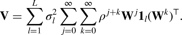
The covariance matrix for Models I and II is $V(\mathbf{Y})={\mathbf{A}}^{-1}({\sigma }_1^2{\mathbf{I}}_N+\mathbf{Z}\mathbf{D}{\mathbf{Z}}^{\mathrm{\top }})({\mathbf{A}}^{-1}{)}^{\mathrm{\top }}$ , where $\mathbf{A}={\mathbf{I}}_N-\rho \mathbf{W}$ . The term ${\sigma }_1^2{\mathbf{I}}_N+\mathbf{Z}\mathbf{D}{\mathbf{Z}}^{\mathrm{\top }}$ can be re-expressed as ${\sigma }_1^2{\mathbf{1}}_1+{\sigma }_2^2{\mathbf{1}}_2+{\sigma }_3^2{\mathbf{1}}_3$ , where ${\mathbf{1}}_l$ is a block-diagonal matrix with the block matrices being matrices of ones and of a size equal to the size of the units at level $l$ . For example, the block matrices in ${\mathbf{1}}_2$ are of a size equal to the households or classes and ${\mathbf{1}}_3$ has blocks of ones of sizes equal to the sizes of areas or schools, and ${\mathbf{1}}_1={\mathbf{I}}_N$ .

The true covariance matrix for Models I and II is:

$$\mathbf{V}={\sigma }_1^2{\mathbf{A}}^{-1}{\mathbf{1}}_1({\mathbf{A}}^{-1}{)}^{\mathrm{\top }}+{\sigma }_2^2{\mathbf{A}}^{-1}{\mathbf{1}}_2({\mathbf{A}}^{-1}{)}^{\mathrm{\top }}+{\sigma }_3^2{\mathbf{A}}^{-1}{\mathbf{1}}_3({\mathbf{A}}^{-1}{)}^{\mathrm{\top }}.$$

A Taylor-series expansion of ${\mathbf{A}}^{-1}$ is ${\mathbf{A}}^{-1}={\mathbf{I}}_N+\sum _{k=1}^{\mathrm{\infty }}{\rho }^k{\mathbf{W}}^k$ . Hence we can write:

$$\mathbf{V}=\sum _{l=1}^L{\sigma }_l^2\sum _{j=0}^{\mathrm{\infty }}\sum _{k=0}^{\mathrm{\infty }}{\rho }^{j+k}{\mathbf{W}}^j{\mathbf{1}}_l({\mathbf{W}}^k{)}^{\mathrm{\top }}.$$

A first-order Taylor series approximation gives:

$$\begin{array}{rl}\mathbf{V}\approx & {\sigma }_1^2{\mathbf{1}}_1+{\sigma }_2^2{\mathbf{1}}_2+{\sigma }_3^2{\mathbf{1}}_3+{\sigma }_1^2\rho (\mathbf{W}{\mathbf{1}}_1+{\mathbf{1}}_1{\mathbf{W}}^{\mathrm{\top }})+{\sigma }_2^2\rho (\mathbf{W}{\mathbf{1}}_2+{\mathbf{1}}_2{\mathbf{W}}^{\mathrm{\top }})\\ & +{\sigma }_3^2\rho (\mathbf{W}{\mathbf{1}}_3+{\mathbf{1}}_3{\mathbf{W}}^{\mathrm{\top }}),\end{array}$$

(12)which has the structure of a standard MLM with additional terms. These terms can produce correlations between people at, below, or above the levels in the MLM, depending on how the network and the levels interact. This makes the theoretical prediction of the effect of omitting a level or the network difficult. In some situations, the network may act much like a level. For example, suppose $\mathbf{W}$ mainly connects people in different groups of level 3 units, then $\mathbf{W}$ can be considered as an approximate level 4 random effects design matrix. When $\mathbf{W}$ connects only people within level $l$ , then $\mathbf{W}{\mathbf{1}}_l+{\mathbf{1}}_l{\mathbf{W}}^{\mathrm{\top }}$ is also of level $l$ . When $\mathbf{W}$ is at level $k$ with $k<l$ , then $\mathbf{W}{\mathbf{1}}_l+{\mathbf{1}}_l{\mathbf{W}}^{\mathrm{\top }}$ refers to level $l$ . In these cases, adding a network to an MLM is similar to adding additional terms to an MLM, possibly affecting multiple levels. If the network is at level $k$ with $k\le L$ , then adding the network implies adding terms from levels $k$ to $L$ , where $L$ is the highest level. When $k>L$ , that is, people in different level $L$ units are connected through the network, then adding a network is like adding another higher level. In these cases, the standard rules for the effect of omitting one or more levels may apply. However, the coefficients for $\mathbf{W}{\mathbf{1}}_l+{\mathbf{1}}_l{\mathbf{W}}^{\mathrm{\top }}$ are products of $\rho$ and ${\sigma }_l^2$ , and are not independent. Due to the dependence of these coefficients, we may not necessarily observe the standard rules when omitting a level or the network.

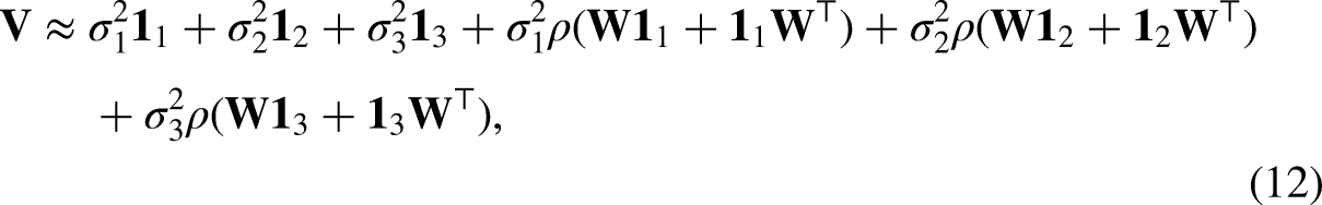
Similarly, for Model III, the first-order approximation is:

$$\mathbf{V}\approx {\sigma }_1^2{\mathbf{1}}_1+{\sigma }_2^2{\mathbf{1}}_2+{\sigma }_3^2{\mathbf{1}}_3+{\sigma }_1^2\rho (\mathbf{W}{\mathbf{1}}_1+{\mathbf{1}}_1{\mathbf{W}}^{\mathrm{\top }}).$$

(13)Here due to the additivity of the random and network effects, the joint dependence issue appears less problematic compared to (12), as there is only one additional term reflecting the network.

Impact of Omitting Network Dependencies

Fixed effects

The impact of omitting the network dependencies on the estimates of the regression parameters differs for the different NAMLMs described in Section “Extended Models That Include Social Network and Group Dependencies: Network Autoregressive Multilevel Models.” For the network effects MLM given by (9), the expectation of the vector of response variables depends on the network dependencies through ${\mathbf{A}}^{-1}$ . Hence the expectation of the OLS estimate of the regression coefficients is $({\mathbf{X}}^{\mathrm{\top }}\mathbf{X}{)}^{-1}{\mathbf{X}}^{\mathrm{\top }}{\mathbf{A}}^{-1}\mathbf{X}\mathit{\beta }$ . Using a first-order Taylor-series approximation, the resulting bias is $({\mathbf{X}}^{\mathrm{\top }}\mathbf{X}{)}^{-1}{\mathbf{X}}^{\mathrm{\top }}\overline{\mathbf{X}}\mathit{\beta }\rho$ and depends on the network contextual variable, $\overline{\mathbf{X}}$ , and $\rho$ . Similar results can be obtained for generalized least squares estimates of $\mathit{\beta }$ .

For the network disturbance Models II and III, the network dependencies do not affect the expectation of the vector of response variables, and so omitting them does not introduce bias into the estimation of the regression coefficients.

Random effects

The covariance matrix for Models I and II can also be re-expressed as

$$\mathbf{V}={\sigma }_1^2{\mathbf{A}}^{-1}{\mathbf{1}}_1({\mathbf{A}}^{-1}{)}^{\mathrm{\top }}+{\sigma }_2^2{\mathbf{A}}^{-1}{\mathbf{1}}_2({\mathbf{A}}^{-1}{)}^{\mathrm{\top }}+{\sigma }_3^2{\mathbf{A}}^{-1}{\mathbf{1}}_3({\mathbf{A}}^{-1}{)}^{\mathrm{\top }}={\sigma }_1^2{\mathbf{M}}_1+{\sigma }_2^2{\mathbf{M}}_2+{\sigma }_3^2{\mathbf{M}}_3,$$

(14)a linear combination of three matrices ${\mathbf{M}}_1$ , ${\mathbf{M}}_2$ , and ${\mathbf{M}}_3$ with ${\mathbf{M}}_l={\mathbf{A}}^{-1}{\mathbf{1}}_l({\mathbf{A}}^{-1}{)}^{\mathrm{\top }}$ . This also shows that the variance associated with each level is modified by the social network dependencies.

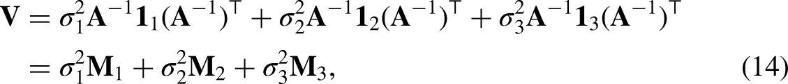
Comparing the true covariance matrix with the one omitting network dependencies, we find that (some of) the estimates of the variance components of the MLM will be overstated, when $\rho >0$ . This is because using a Taylor-series expansion of ${\mathbf{A}}^{-1}$ , it can be shown that $\mathbf{V}\ge {\sigma }_1^2{\mathbf{1}}_1+{\sigma }_2^2{\mathbf{1}}_2+{\sigma }_3^2{\mathbf{1}}_3$ for $\rho \ge 0$ , because ${\mathbf{M}}_l\ge {\mathbf{1}}_l$ . This means that when using the true values of ${\sigma }_1^2$ , ${\sigma }_2^2$ and ${\sigma }_3^2$ and ignoring the network, the implied variance, ${\sigma }_1^2{\mathbf{1}}_1+{\sigma }_2^2{\mathbf{1}}_2+{\sigma }_3^2{\mathbf{1}}_3$ , is less than the true variance $\mathbf{V}$ . Because ${\mathbf{1}}_l\ge 0$ , then at least some of the estimates, ${\hat{\sigma }}_l^2$ , of the variance components omitting network dependencies will be over-estimated compared to the true ${\sigma }_l^2$ of the full model to compensate for the otherwise underestimated variance $\mathbf{V}$ . Only for the unusual case of negative $\rho$ can under-estimation occur for some levels.

The online Appendix C provides some details of this argument. Generally, an analysis that does not account for the network gives estimates of the variance components that are too large, when $\rho >0$ . Using only the first-order term in the Taylor-series ${\mathbf{M}}_l\approx (\mathbf{I}+\rho \mathbf{W}){\mathbf{1}}_l(\mathbf{I}+\rho \mathbf{W}{)}^{\mathrm{\top }}\approx {\mathbf{1}}_l+\rho (\mathbf{W}{\mathbf{1}}_l+{\mathbf{1}}_l{\mathbf{W}}^{\mathrm{\top }})$ , which suggests that the amount by which ${\sigma }_l^2$ is over-estimated depends on $\rho$ and how the level and network are related as reflected by $\mathbf{W}{\mathbf{1}}_l+{\mathbf{1}}_l{\mathbf{W}}^{\mathrm{\top }}$ .

When using the arguments of Section “Re-expressing the Covariance Matrix of NAMLMs,” the additional terms refer to a certain level or levels. Ignoring a network should lead to different variance estimate at the affected level and at adjacent levels and likewise for SEs. For example, when the omitted network is above the highest level (level 3), then the level 3 variance estimate component should change. Since the fixed intercept can be considered as a level 4 predictor, then the SE of the fixed intercept should also be affected. However, due to the joint dependence of $\rho$ and ${\sigma }_l^2$ , other levels may still be affected.

For Model III, similar results can be obtained by noting that for this model:

$$\mathbf{V}={\sigma }_1^2{\mathbf{M}}_1+{\sigma }_2^2{\mathbf{1}}_2+{\sigma }_3^2{\mathbf{1}}_3.$$

(15)For this model, only the variance associated with the individual level is modified by the social network dependencies.

Impact of Omitting Multilevel Dependencies

To assess the impact of omitting a level in the NAMLMs the method of moments is applied, following Berkhof and Kampen (2004). First let us assume the network parameter can be estimated consistently, which may not always hold, but the simulation study (Section “Example With School Data”) indicates that the estimates of the network parameters are roughly the same regardless of the number of levels used in the model. For Model II, the residuals are $\mathbf{r}=\mathbf{Y}-\mathbf{X}\hat{\mathit{\beta }}$ where $\hat{\mathit{\beta }}={\hat{\mathit{\beta }}}_{OLS}$ . Then $\mathbf{r}$ is approximately zero mean normal with covariance $\mathbf{V}={\sigma }_1^2{\mathbf{A}}^{-1}({\mathbf{A}}^{-1}{)}^{\mathrm{\top }}+{\sigma }_2^2{\mathbf{A}}^{-1}{\mathbf{1}}_2({\mathbf{A}}^{-1}{)}^{\mathrm{\top }}+{\sigma }_3^2{\mathbf{A}}^{-1}{\mathbf{1}}_3({\mathbf{A}}^{-1}{)}^{\mathrm{\top }}$ . Let $\tilde{\mathbf{r}}=\mathbf{A}(\rho )\mathbf{r}$ . Provided a consistent estimate of $\rho$ exists (or alternatively the estimate of $\rho$ is the same when a level is ignored compared to the full model), the variance of $\tilde{\mathbf{r}}$ is approximately ${\sigma }_1^2{\mathbf{1}}_1+{\sigma }_2^2{\mathbf{1}}_2+{\sigma }_3^2{\mathbf{1}}_3$ (consistency of $\hat{\rho }$ implies consistency of $\widehat{\tilde{\mathbf{r}}}$ ), that is, the transformed residuals have the same form as those from a standard MLM. Estimation of the random intercept variances can now be based on the transformed residuals $\tilde{\mathbf{r}}$ . Therefore, the same rules for omitting a level in a MLM apply, see for example, Tranmer and Steel (2001) and Berkhof and Kampen (2004). For example, omitting the area level will give an inflated estimate of the household-level variance, whereas omitting the household level will lead to increased area-level and individual-level variances. Also, similar rules apply to SEs, as for standard MLMs. If $\rho$ is estimated correctly then these rules apply.

However, as we have seen in Section “Re-expressing the Covariance Matrix of NAMLMs” by re-expressing the covariance (12), adding the network to a standard MLM is equivalent to adding other terms related to existing or higher level(s) and the coefficients of these terms are functions of $\rho$ and ${\sigma }_l^2$ . Ignoring the joint dependence, we would expect that ignoring a level only affects estimates of the same level or adjacent levels. For example, if the network is at level $4$ and level 3 is ignored, then we would expect level 2 and level 3 variance estimates to be affected and also the $\rho$ estimate, but not level 1 estimates, that is, ${\sigma }_1^2$ and SEs of level 1 predictors to be unaffected, since level 1 is not adjacent to level 3. Using that argument, we would expect the level 4 estimate to change, that is, we would expect $\hat{\rho }$ to change as well, and hence the above situation ( $\hat{\rho }$ to remain the same) is not always valid.

Simulation Study

Setup of Simulation Study

In this section, we consider a situation involving people within households, which are located within areas and are involved in a social network. To assess the impact of omitting one of the components (network, household, and area) of the model, we conduct a simulation study.

For Models I, II and III, we randomly generate 200 areas, and each area has 10 households. The size for each of the 10 households is randomly chosen using the probabilities 0.294, 0.332, 0.136, 0.146, 0.063, 0.020, 0.006, and 0.002 for household sizes 1,2,3, …, 8. Those probabilities are taken from the Household, Income and Labor Dynamics in Australia (HILDA) survey using the observed frequencies from wave 8 (2008) (Summerfield et al. 2015). The simulations take the number of households in an area as fixed, which is often the case in social surveys. The theoretical results do not assume groups of equal size, nor does the analysis of real data in Section “Example With School Data.”

The data are generated under Models I, II, and III to assess the effect of omitting any combination of the three components. The variance parameters are set to ${\sigma }_1^2=1.0$ (individuals), ${\sigma }_2^2=0.3$ (households), and ${\sigma }_3^2=0.1$ (areas). As covariates we consider a household level covariate represented by $X^{(2)}$ , an area level covariate $X^{(3)}$ , and a individual-level covariate $X^{(1)}$ . The models also include an intercept, so $\mathbf{x}=(1,X^{(1)},X^{(2)},X^{(3)}{)}^{\mathrm{\top }}$ , and $\mathit{\beta }=(-1,2,0.2,0.3{)}^{\mathrm{\top }}$ .

The covariates were all generated from the standard normal distribution, that is, $X^{(k)}\sim N(0,1)$ . To assess the effect of a positive and a negative network parameter $\rho$ , we consider the values $\rho =0.3$ and $\rho =-0.3$ for all three models. The number of simulated data sets is 10,000. The empirical mean for the 10,000 simulations of the estimates of the fixed effects $\mathit{\beta }$ , the random effects parameters ${\sigma }_l^2$ , $l=1,2,3$ , and $\rho$ were calculated, as well as the empirical standard deviations (SDs) of the estimates of the fixed effects parameters. These means and SDs of the regression coefficient estimates give the expectation and the true SEs of the estimates of the regression coefficients, respectively.

In practice, the SEs of the regression coefficients will be estimated for a model or sub-model using the available data. The SE estimates may be biased and not estimate the true SEs well when the network or one or more levels are omitted, which can affect statistical inferences. The effect of omitting the network or levels on statistical inference for the regression coefficients was evaluated in the simulations by examining the relative bias of the SE estimates and coverage of the associated nominal 95 percent confidence intervals (i.e., proportion of times the true regression parameter is included). SEs were estimated in a standard way, using the inverse of the Fisher information matrix (see the online Appendix B.2) and confidence intervals constructed by adding and subtracting 1.96 times the estimated SE to the estimated regression coefficient. A negative bias will lead to underestimation of the true SEs and overstate the statistical significance (i.e., p-value too small) and reduced coverage of the true regression coefficients by the associated 95 percent confidence intervals.

For each of Models I, II, and III, results were generated for the full model and for all submodels, that is, for any combination of the components referring to the household and area level and the network. That means in total $2^3=8$ submodels (including the full model) were fitted for each data set for each of the three NAMLMs, for the parameter values specified. Further simulation studies could use other parameter values.

The network comprising all individuals was generated by an ERGM (Snijders et al. 2006) with a GWESP (geometrically weighted edgewise shared partner) statistic, or sometimes called distribution, and an edge statistic with the parameters set to $1$ and $-4$ to have on average approximately 4.5 links per individual. This was done using the ergm R package (Handcock et al. 2010). We also considered a scenario in which the network was limited to within areas, similar to the inter-school network in Section “Example With School Data.” For this scenario, the two parameters were set to $1$ and $-2$ in order to have roughly the same number of links for both cases.

Results of Simulation Study

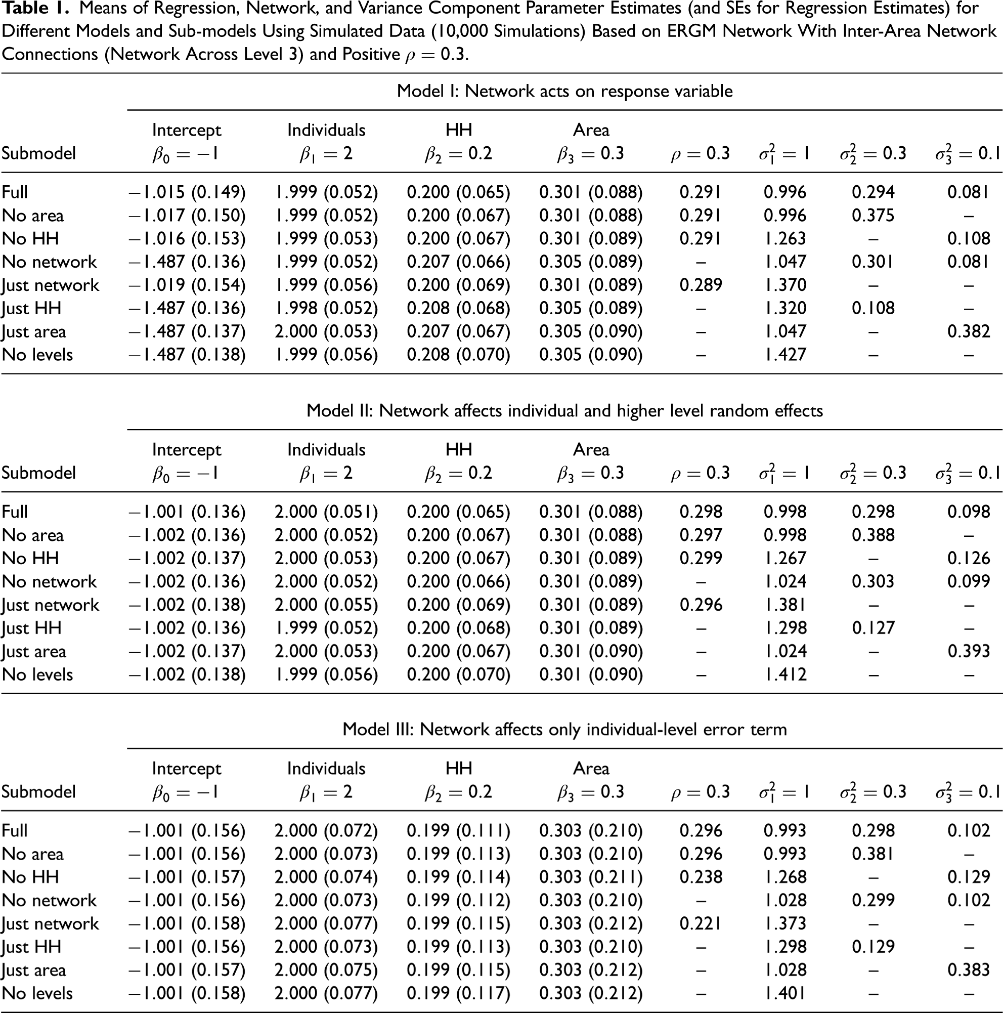
Table 1 shows the results for the three models with $\rho =0.3$ and the network comprising all individuals, allowing network dependencies between individuals in different areas. Table 2 shows the results when $\rho =0.3$ but with the network connections restricted to within areas. Tables S1 and S2 (see Supplemental Material) are similar to Tables 1 and 2, except that $\rho =-0.3$ is negative, which is a less common situation.

Table 1.

Means of Regression, Network, and Variance Component Parameter Estimates (and SEs for Regression Estimates) for Different Models and Sub-models Using Simulated Data (10,000 Simulations) Based on ERGM Network With Inter-Area Network Connections (Network Across Level 3) and Positive $\rho =0.3$ .

	Model I: Network acts on response variable
	Intercept	Individuals	HH	Area
Submodel	${\beta }_0=-1$	${\beta }_1=2$	${\beta }_2=0.2$	${\beta }_3=0.3$	$\rho =0.3$	${\sigma }_1^2=1$	${\sigma }_2^2=0.3$	${\sigma }_3^2=0.1$
Full	−1.015 (0.149)	1.999 (0.052)	0.200 (0.065)	0.301 (0.088)	0.291	0.996	0.294	0.081
No area	−1.017 (0.150)	1.999 (0.052)	0.200 (0.067)	0.301 (0.088)	0.291	0.996	0.375	–
No HH	−1.016 (0.153)	1.999 (0.053)	0.200 (0.067)	0.301 (0.089)	0.291	1.263	–	0.108
No network	−1.487 (0.136)	1.999 (0.052)	0.207 (0.066)	0.305 (0.089)	–	1.047	0.301	0.081
Just network	−1.019 (0.154)	1.999 (0.056)	0.200 (0.069)	0.301 (0.089)	0.289	1.370	–	–
Just HH	−1.487 (0.136)	1.998 (0.052)	0.208 (0.068)	0.305 (0.089)	–	1.320	0.108	–
Just area	−1.487 (0.137)	2.000 (0.053)	0.207 (0.067)	0.305 (0.090)	–	1.047	–	0.382
No levels	−1.487 (0.138)	1.999 (0.056)	0.208 (0.070)	0.305 (0.090)	–	1.427	–	–

	Model II: Network affects individual and higher level random effects
	Intercept	Individuals	HH	Area
Submodel	${\beta }_0=-1$	${\beta }_1=2$	${\beta }_2=0.2$	${\beta }_3=0.3$	$\rho =0.3$	${\sigma }_1^2=1$	${\sigma }_2^2=0.3$	${\sigma }_3^2=0.1$
Full	−1.001 (0.136)	2.000 (0.051)	0.200 (0.065)	0.301 (0.088)	0.298	0.998	0.298	0.098
No area	−1.002 (0.136)	2.000 (0.052)	0.200 (0.067)	0.301 (0.088)	0.297	0.998	0.388	–
No HH	−1.002 (0.137)	2.000 (0.053)	0.200 (0.067)	0.301 (0.089)	0.299	1.267	–	0.126
No network	−1.002 (0.136)	2.000 (0.052)	0.200 (0.066)	0.301 (0.089)	–	1.024	0.303	0.099
Just network	−1.002 (0.138)	2.000 (0.055)	0.200 (0.069)	0.301 (0.089)	0.296	1.381	–	–
Just HH	−1.002 (0.136)	1.999 (0.052)	0.200 (0.068)	0.301 (0.089)	–	1.298	0.127	–
Just area	−1.002 (0.137)	2.000 (0.053)	0.200 (0.067)	0.301 (0.090)	–	1.024	–	0.393
No levels	−1.002 (0.138)	1.999 (0.056)	0.200 (0.070)	0.301 (0.090)	–	1.412	–	–

	Model III: Network affects only individual-level error term
	Intercept	Individuals	HH	Area
Submodel	${\beta }_0=-1$	${\beta }_1=2$	${\beta }_2=0.2$	${\beta }_3=0.3$	$\rho =0.3$	${\sigma }_1^2=1$	${\sigma }_2^2=0.3$	${\sigma }_3^2=0.1$
Full	−1.001 (0.156)	2.000 (0.072)	0.199 (0.111)	0.303 (0.210)	0.296	0.993	0.298	0.102
No area	−1.001 (0.156)	2.000 (0.073)	0.199 (0.113)	0.303 (0.210)	0.296	0.993	0.381	–
No HH	−1.001 (0.157)	2.000 (0.074)	0.199 (0.114)	0.303 (0.211)	0.238	1.268	–	0.129
No network	−1.001 (0.156)	2.000 (0.073)	0.199 (0.112)	0.303 (0.210)	–	1.028	0.299	0.102
Just network	−1.001 (0.158)	2.000 (0.077)	0.199 (0.115)	0.303 (0.212)	0.221	1.373	–	–
Just HH	−1.001 (0.156)	2.000 (0.073)	0.199 (0.113)	0.303 (0.210)	–	1.298	0.129	–
Just area	−1.001 (0.157)	2.000 (0.075)	0.199 (0.115)	0.303 (0.212)	–	1.028	–	0.383
No levels	−1.001 (0.158)	2.000 (0.077)	0.199 (0.117)	0.303 (0.212)	–	1.401	–	–

Table 2.

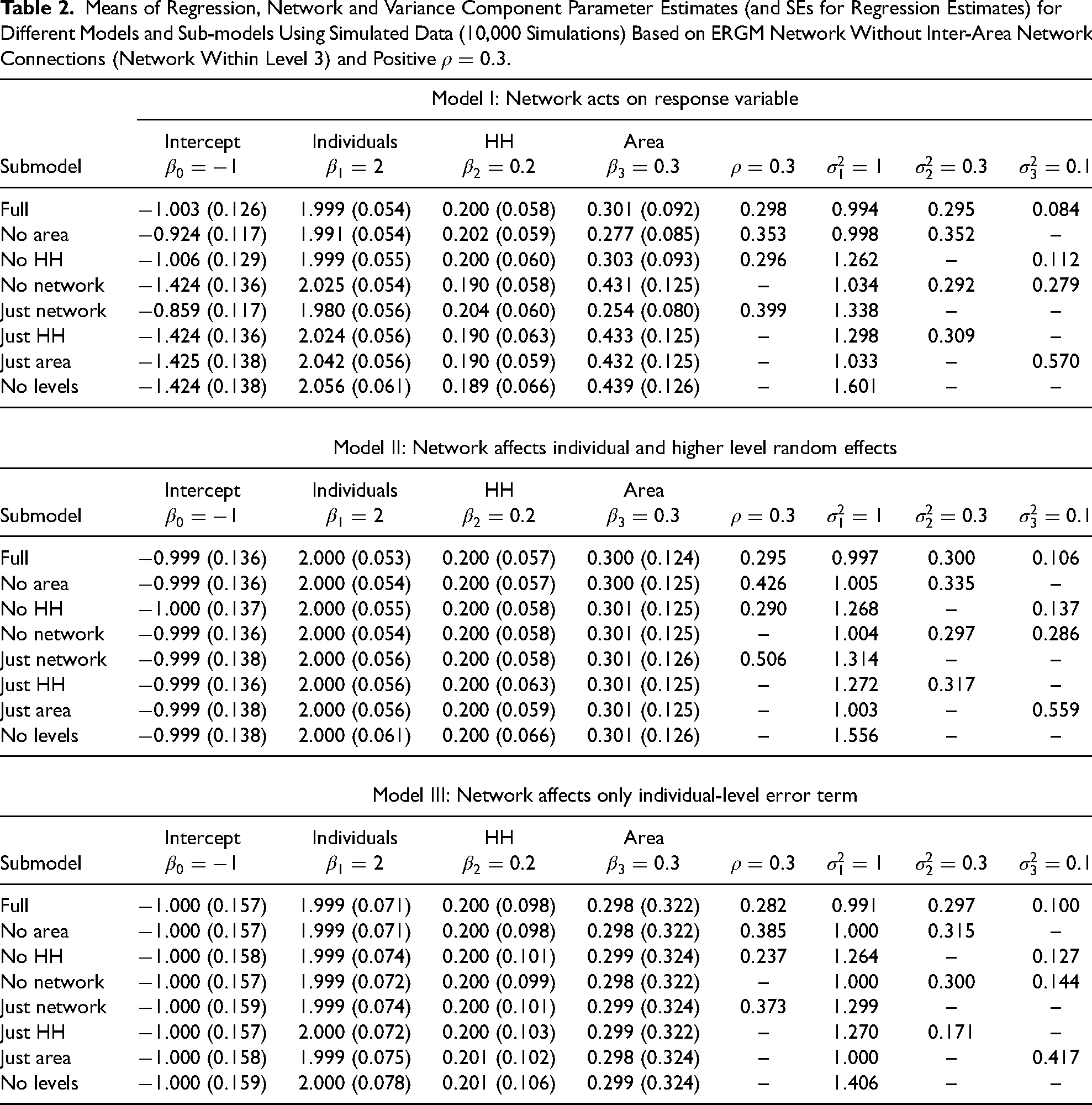
Means of Regression, Network and Variance Component Parameter Estimates (and SEs for Regression Estimates) for Different Models and Sub-models Using Simulated Data (10,000 Simulations) Based on ERGM Network Without Inter-Area Network Connections (Network Within Level 3) and Positive $\rho =0.3$ .

	Model I: Network acts on response variable
	Intercept	Individuals	HH	Area
Submodel	${\beta }_0=-1$	${\beta }_1=2$	${\beta }_2=0.2$	${\beta }_3=0.3$	$\rho =0.3$	${\sigma }_1^2=1$	${\sigma }_2^2=0.3$	${\sigma }_3^2=0.1$
Full	−1.003 (0.126)	1.999 (0.054)	0.200 (0.058)	0.301 (0.092)	0.298	0.994	0.295	0.084
No area	−0.924 (0.117)	1.991 (0.054)	0.202 (0.059)	0.277 (0.085)	0.353	0.998	0.352	–
No HH	−1.006 (0.129)	1.999 (0.055)	0.200 (0.060)	0.303 (0.093)	0.296	1.262	–	0.112
No network	−1.424 (0.136)	2.025 (0.054)	0.190 (0.058)	0.431 (0.125)	–	1.034	0.292	0.279
Just network	−0.859 (0.117)	1.980 (0.056)	0.204 (0.060)	0.254 (0.080)	0.399	1.338	–	–
Just HH	−1.424 (0.136)	2.024 (0.056)	0.190 (0.063)	0.433 (0.125)	–	1.298	0.309	–
Just area	−1.425 (0.138)	2.042 (0.056)	0.190 (0.059)	0.432 (0.125)	–	1.033	–	0.570
No levels	−1.424 (0.138)	2.056 (0.061)	0.189 (0.066)	0.439 (0.126)	–	1.601	–	–

	Model II: Network affects individual and higher level random effects
	Intercept	Individuals	HH	Area
Submodel	${\beta }_0=-1$	${\beta }_1=2$	${\beta }_2=0.2$	${\beta }_3=0.3$	$\rho =0.3$	${\sigma }_1^2=1$	${\sigma }_2^2=0.3$	${\sigma }_3^2=0.1$
Full	−0.999 (0.136)	2.000 (0.053)	0.200 (0.057)	0.300 (0.124)	0.295	0.997	0.300	0.106
No area	−0.999 (0.136)	2.000 (0.054)	0.200 (0.057)	0.300 (0.125)	0.426	1.005	0.335	–
No HH	−1.000 (0.137)	2.000 (0.055)	0.200 (0.058)	0.301 (0.125)	0.290	1.268	–	0.137
No network	−0.999 (0.136)	2.000 (0.054)	0.200 (0.058)	0.301 (0.125)	–	1.004	0.297	0.286
Just network	−0.999 (0.138)	2.000 (0.056)	0.200 (0.058)	0.301 (0.126)	0.506	1.314	–	–
Just HH	−0.999 (0.136)	2.000 (0.056)	0.200 (0.063)	0.301 (0.125)	–	1.272	0.317	–
Just area	−0.999 (0.138)	2.000 (0.056)	0.200 (0.059)	0.301 (0.125)	–	1.003	–	0.559
No levels	−0.999 (0.138)	2.000 (0.061)	0.200 (0.066)	0.301 (0.126)	–	1.556	–	–

	Model III: Network affects only individual-level error term
	Intercept	Individuals	HH	Area
Submodel	${\beta }_0=-1$	${\beta }_1=2$	${\beta }_2=0.2$	${\beta }_3=0.3$	$\rho =0.3$	${\sigma }_1^2=1$	${\sigma }_2^2=0.3$	${\sigma }_3^2=0.1$
Full	−1.000 (0.157)	1.999 (0.071)	0.200 (0.098)	0.298 (0.322)	0.282	0.991	0.297	0.100
No area	−1.000 (0.157)	1.999 (0.071)	0.200 (0.098)	0.298 (0.322)	0.385	1.000	0.315	–
No HH	−1.000 (0.158)	1.999 (0.074)	0.200 (0.101)	0.299 (0.324)	0.237	1.264	–	0.127
No network	−1.000 (0.157)	1.999 (0.072)	0.200 (0.099)	0.298 (0.322)	–	1.000	0.300	0.144
Just network	−1.000 (0.159)	1.999 (0.074)	0.200 (0.101)	0.299 (0.324)	0.373	1.299	–	–
Just HH	−1.000 (0.157)	2.000 (0.072)	0.200 (0.103)	0.299 (0.322)	–	1.270	0.171	–
Just area	−1.000 (0.158)	1.999 (0.075)	0.201 (0.102)	0.298 (0.324)	–	1.000	–	0.417
No levels	−1.000 (0.159)	2.000 (0.078)	0.201 (0.106)	0.299 (0.324)	–	1.406	–	–

Effect of omitting levels on estimates of variance components and network parameter

The results in Table 1 show that when the social network is included, omitting one or more levels has a very similar effect on the estimates of the remaining variance components as in a standard MLM described in Section “Re-expressing the Covariance Matrix of NAMLMs.” There is no appreciable effect on the estimation of the network parameter, $\rho$ , except in Model III, where there is some reduction when the household level is ignored.

Effect of omitting network dependencies on estimates of variance components

When no network is included, there is no appreciable effect on the estimates of the variance components when all are included. However, the omission of the area level component decreases the household level and increases the individual-level variance components considerably. When the household level is omitted, the area-level variance component increases considerably. This does not happen when the network is included, suggesting that it plays a role in the effects of omitting a level.

Effect of omitting network dependencies or levels on estimates of regression parameters

The mean of the estimates of the regression parameters is not affected at all by omitting the social network or levels in Models II and III. Even in Model I, where an effect might be expected when the network is omitted, there is no impact on the individual-level regression parameter and very small effects for the regression parameters of household and area level covariates, although the estimation of the intercept is affected.

Effect on SEs and inferences for regression coefficients

The SEs of the regression coefficients estimates shown in Table 1 reflect the loss of efficiency as levels or the social network are omitted from the variance structure, V(Y), used in estimating these coefficients. For a particular submodel, the loss of efficiency is the ratio of the square of the SE to that of the full model (i.e., ratio of variances). When only the network is omitted, so a standard MLM is fitted, the SEs are essentially the same as for the full model and there is no loss of efficiency. The SEs are the highest when all levels and the network are omitted, resulting in the efficiency losses ranging between 3 percent and 21 percent. These SEs are close to the case when only the network is included. In general, provided at least one of the household or area level is included any efficiency loss is small. An exception to these results is the intercept in Model I, where omitting the network leads to smaller SEs. In all cases, the SEs for the regression coefficients obtained using Model III are appreciably larger than for Models I and II, which are similar to each other.

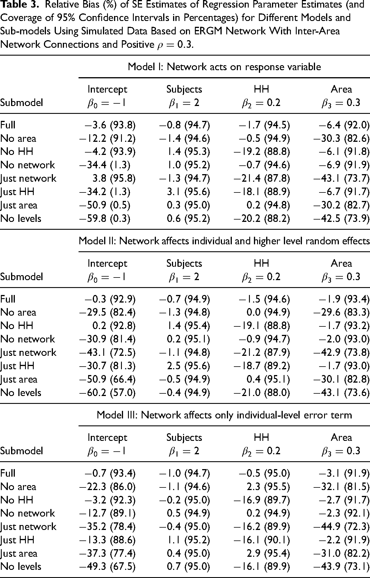
The relative biases of the SE estimates and the coverage of the associated 95 percent confidence intervals are given in Table 3 for the simulations allowing network dependencies between individuals in different areas, corresponding to Table 1. Poor coverage can arise due to underestimation of the SE and/or bias in the estimate of the regression coefficients. For the individual-level regression coefficients, the relative bias of the SE estimates is very small and the coverage is always close to the nominal 95 percent (i.e., 5 percent significance level) for all models or submodels used, including the submodel omitting the network and levels. For the household and area-level regression coefficients the omission of the network has a little or no effect on coverage provided the levels are included. Including only the network leads to appreciable negative relative biases in the SE estimates and poor coverage. Omitting only the household (area) leads to negative biases in the SE estimates and poor coverage of the household (area)-level regression coefficient. When the network is omitted, omitting the household (area) leads to a poor coverage for the area (household) regression coefficient. For the intercept in Models II and III, there is a large negative relative bias in the estimated SEs leading to a poor coverage, except for the full model or where the household is omitted. For Model I, even worse coverages are obtained because of the bias in the estimation of the intercept when there is no network already shown in Table 1, combined with underestimation of the SEs. We see that the expectation of the estimates of the regression coefficients and inferences about the individual-level regression coefficient are generally not affected by the omission of the network or levels. However, the inferences about the household and area-level regression coefficients and the intercept can be affected due to the underestimation of the SEs, which leads to overstating the statistical significance and poor coverage.

Table 3.

Relative Bias (%) of SE Estimates of Regression Parameter Estimates (and Coverage of 95% Confidence Intervals in Percentages) for Different Models and Sub-models Using Simulated Data Based on ERGM Network With Inter-Area Network Connections and Positive $\rho =0.3$ .

	Model I: Network acts on response variable
	Intercept	Subjects	HH	Area
Submodel	${\beta }_0=-1$	${\beta }_1=2$	${\beta }_2=0.2$	${\beta }_3=0.3$
Full	−3.6 (93.8)	−0.8 (94.7)	−1.7 (94.5)	−6.4 (92.0)
No area	−12.2 (91.2)	−1.4 (94.6)	−0.5 (94.9)	−30.3 (82.6)
No HH	−4.2 (93.9)	1.4 (95.3)	−19.2 (88.8)	−6.1 (91.8)
No network	−34.4 (1.3)	1.0 (95.2)	−0.7 (94.6)	−6.9 (91.9)
Just network	3.8 (95.8)	−1.3 (94.7)	−21.4 (87.8)	−43.1 (73.7)
Just HH	−34.2 (1.3)	3.1 (95.6)	−18.1 (88.9)	−6.7 (91.7)
Just area	−50.9 (0.5)	0.3 (95.0)	0.2 (94.8)	−30.2 (82.7)
No levels	−59.8 (0.3)	0.6 (95.2)	−20.2 (88.2)	−42.5 (73.9)
	Model II: Network affects individual and higher level random effects
	Intercept	Subjects	HH	Area
Submodel	${\beta }_0=-1$	${\beta }_1=2$	${\beta }_2=0.2$	${\beta }_3=0.3$
Full	−0.3 (92.9)	−0.7 (94.9)	−1.5 (94.6)	−1.9 (93.4)
No area	−29.5 (82.4)	−1.3 (94.8)	0.0 (94.9)	−29.6 (83.3)
No HH	0.2 (92.8)	1.4 (95.4)	−19.1 (88.8)	−1.7 (93.2)
No network	−30.9 (81.4)	0.2 (95.1)	−0.9 (94.7)	−2.0 (93.0)
Just network	−43.1 (72.5)	−1.1 (94.8)	−21.2 (87.9)	−42.9 (73.8)
Just HH	−30.7 (81.3)	2.5 (95.6)	−18.7 (89.2)	−1.7 (93.0)
Just area	−50.9 (66.4)	−0.5 (94.9)	0.4 (95.1)	−30.1 (82.8)
No levels	−60.2 (57.0)	−0.4 (94.9)	−21.0 (88.0)	−43.1 (73.6)
	Model III: Network affects only individual-level error term
	Intercept	Subjects	HH	Area
Submodel	${\beta }_0=-1$	${\beta }_1=2$	${\beta }_2=0.2$	${\beta }_3=0.3$
Full	−0.7 (93.4)	−1.0 (94.7)	−0.5 (95.0)	−3.1 (91.9)
No area	−22.3 (86.0)	−1.1 (94.6)	2.3 (95.5)	−32.1 (81.5)
No HH	−3.2 (92.3)	−0.2 (95.0)	−16.9 (89.7)	−2.7 (91.7)
No network	−12.7 (89.1)	0.5 (94.9)	0.2 (94.9)	−2.3 (92.1)
Just network	−35.2 (78.4)	−0.4 (95.0)	−16.2 (89.9)	−44.9 (72.3)
Just HH	−13.3 (88.6)	1.1 (95.2)	−16.1 (90.1)	−2.2 (91.9)
Just area	−37.3 (77.4)	0.4 (95.0)	2.9 (95.4)	−31.0 (82.2)
No levels	−49.3 (67.5)	0.7 (95.0)	−16.1 (89.9)	−43.9 (73.1)

Results when social network contained within areas

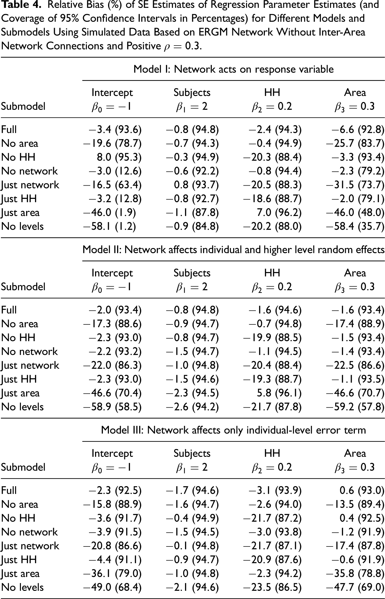
The results in Table 2 correspond to the case when the social network is contained within the area level, but can still connect different households. Many of the observations made for Table 1 apply, however, there are some noteworthy differences associated with the interplay between the network and the area-level effect. When the area level is omitted, the estimate of $\rho$ increases considerably. When the network is omitted, the estimate of the area-level variance component increases considerably. Also, omitting the network increases the regression coefficient for the area-level covariate in Model I. These results arise because in this case, the network and area effects both produce within-area correlations. For the SEs, the effect of using different types of models and omitted components of variance structure are similar to those shown in Table 1. The relative bias of the estimated SEs and the associated coverage of the 95 percent confidence intervals are given in Table 4. The general conclusions are similar to those in Table 3. There are some additional cases of poor coverage in Model I: in the estimation of the individual-level regression coefficient with no network effect or levels, or just an area effect, and also in the area-level regression coefficient when there is no network or just household, which is due to the bias in the coefficient noted previously.

Table 4.

Relative Bias (%) of SE Estimates of Regression Parameter Estimates (and Coverage of 95% Confidence Intervals in Percentages) for Different Models and Submodels Using Simulated Data Based on ERGM Network Without Inter-Area Network Connections and Positive $\rho =0.3$ .

	Model I: Network acts on response variable
	Intercept	Subjects	HH	Area
Submodel	${\beta }_0=-1$	${\beta }_1=2$	${\beta }_2=0.2$	${\beta }_3=0.3$
Full	−3.4 (93.6)	−0.8 (94.8)	−2.4 (94.3)	−6.6 (92.8)
No area	−19.6 (78.7)	−0.7 (94.3)	−0.4 (94.9)	−25.7 (83.7)
No HH	8.0 (95.3)	−0.3 (94.9)	−20.3 (88.4)	−3.3 (93.4)
No network	−3.0 (12.6)	−0.6 (92.2)	−0.8 (94.4)	−2.3 (79.2)
Just network	−16.5 (63.4)	0.8 (93.7)	−20.5 (88.3)	−31.5 (73.7)
Just HH	−3.2 (12.8)	−0.8 (92.7)	−18.6 (88.7)	−2.0 (79.1)
Just area	−46.0 (1.9)	−1.1 (87.8)	7.0 (96.2)	−46.0 (48.0)
No levels	−58.1 (1.2)	−0.9 (84.8)	−20.2 (88.0)	−58.4 (35.7)
	Model II: Network affects individual and higher level random effects
	Intercept	Subjects	HH	Area
Submodel	${\beta }_0=-1$	${\beta }_1=2$	${\beta }_2=0.2$	${\beta }_3=0.3$
Full	−2.0 (93.4)	−0.8 (94.8)	−1.6 (94.6)	−1.6 (93.4)
No area	−17.3 (88.6)	−0.9 (94.7)	−0.7 (94.8)	−17.4 (88.9)
No HH	−2.3 (93.0)	−0.8 (94.7)	−19.9 (88.5)	−1.5 (93.4)
No network	−2.2 (93.2)	−1.5 (94.7)	−1.1 (94.5)	−1.4 (93.4)
Just network	−22.0 (86.3)	−1.0 (94.8)	−20.4 (88.4)	−22.5 (86.6)
Just HH	−2.3 (93.0)	−1.5 (94.6)	−19.3 (88.7)	−1.1 (93.5)
Just area	−46.6 (70.4)	−2.3 (94.5)	5.8 (96.1)	−46.6 (70.7)
No levels	−58.9 (58.5)	−2.6 (94.2)	−21.7 (87.8)	−59.2 (57.8)
	Model III: Network affects only individual-level error term
	Intercept	Subjects	HH	Area
Submodel	${\beta }_0=-1$	${\beta }_1=2$	${\beta }_2=0.2$	${\beta }_3=0.3$
Full	−2.3 (92.5)	−1.7 (94.6)	−3.1 (93.9)	0.6 (93.0)
No area	−15.8 (88.9)	−1.6 (94.7)	−2.6 (94.0)	−13.5 (89.4)
No HH	−3.6 (91.7)	−0.4 (94.9)	−21.7 (87.2)	0.4 (92.5)
No network	−3.9 (91.5)	−1.5 (94.5)	−3.0 (93.8)	−1.2 (91.9)
Just network	−20.8 (86.6)	−0.1 (94.8)	−21.7 (87.1)	−17.4 (87.8)
Just HH	−4.4 (91.1)	−0.9 (94.7)	−20.9 (87.6)	−0.6 (91.9)
Just area	−36.1 (79.0)	−1.0 (94.8)	−2.3 (94.2)	−35.8 (78.8)
No levels	−49.0 (68.4)	−2.1 (94.6)	−23.5 (86.5)	−47.7 (69.0)

Results with negative $\rho$

In Supplemental Table S1, where $\rho$ is negative and there are inter-area connections, the results are similar to Table 1 for the estimates of the regression coefficients, the network parameter, variance components, and the SEs. The estimates of the regression coefficient are not affected by omitting levels or the network. Omitting a level results in increases in the variance component for the levels included in the model. Estimation of $\rho$ is not substantially affected by the levels included, and omission of the network does not affect the estimation of the other variance components when all are included. As in Table 1 when no network is included, the omission of the area-level component decreases the household level and increases the individual-level variance component. When the household level is omitted, the area-level variance component increases considerably. As in Table 1 this does not happen when the network is included. When the social network is contained within the area level and $\rho$ is negative, the interplay between the network and area-level effect has a dampening effect when either is omitted, as shown in Supplemental Table S2. Omitting the area-level effect contributes some positive correlations within the network that is contained within the areas, and this works against the negative autocorrelation to move the estimate of $\rho$ towards zero, or to make it positive. Omitting the network in this case, the means some negative correlations are influencing the within area correlations, reducing the estimate of the area-level variance component. The relative biases of the SE estimates and associated coverage are given in Supplemental Table S3 for the case where there are inter-area network connections, and in Supplemental Table S4 when the network connections are contained within areas. The general conclusions are the same as for the corresponding case of positive $\rho$ .

When $\rho =0$ or $\rho >0.3$

We have not shown simulation study results for $\rho =0$ (no network effects) and for larger values of $\rho$ , for example, $\rho =0.7$ . However, the results presented in the tables (including Tables 5 and 6 for the data set considered in Section “Example With School Data”) suggest what happens in both cases. When $\rho =0$ , the estimated $\rho$ will be, on average, near zero, but for a given data set, $\hat{\rho }$ is almost certainly non-zero. So we can compare the rows “no network” ( $\hat{\rho }=0$ ) with “full” ( $\hat{\rho }\ne 0$ ) to see the effect of incorporating the network, that is, some or all variance components will generally decrease (more so if $\hat{\rho }>0$ ). The case of $\rho >0.3$ is similar to the case $\rho =0.3$ , only the effects are larger. Since the matrices ${\mathbf{M}}_l$ depend on $\rho$ and the size of the elements of ${\mathbf{M}}_l$ relative to ${\mathbf{1}}_l$ will increase with $\rho$ (for $\rho >0$ ), the effects relating to the network will generally be larger. For example, omitting the network leads to larger increases in the estimated variance components.

Table 5.

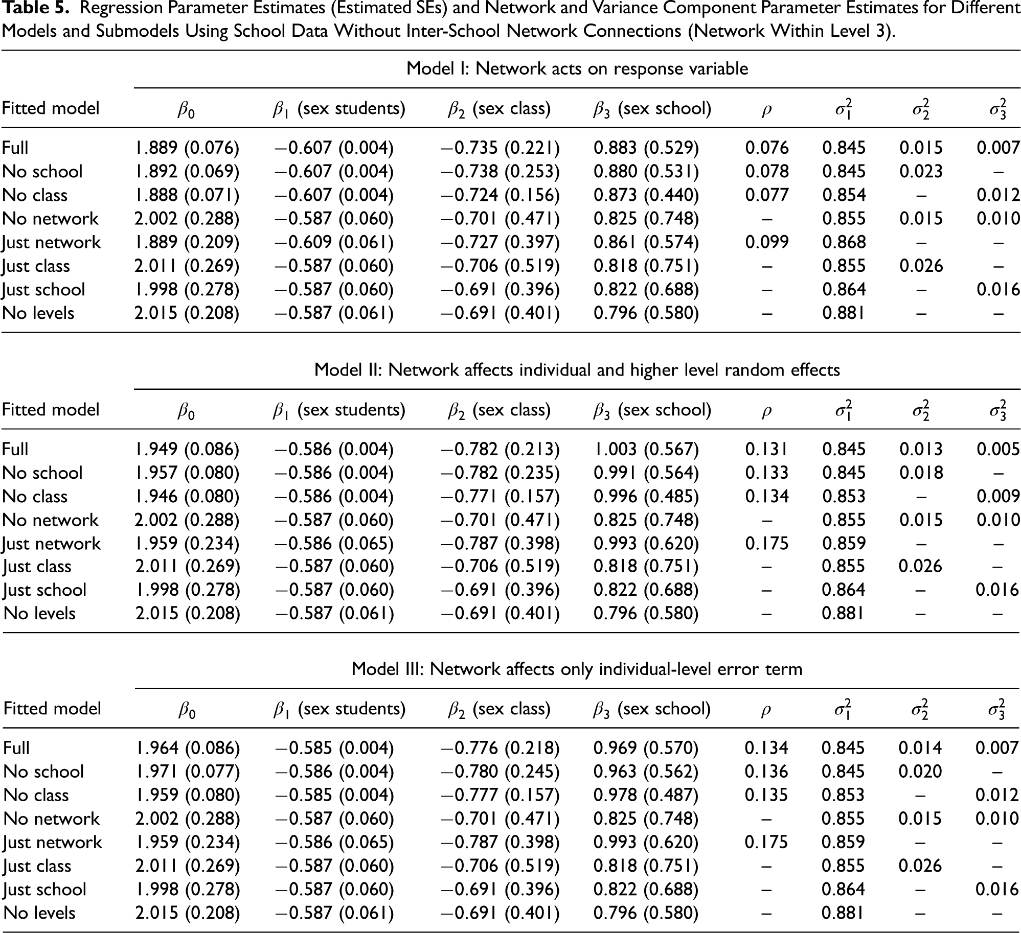
Regression Parameter Estimates (Estimated SEs) and Network and Variance Component Parameter Estimates for Different Models and Submodels Using School Data Without Inter-School Network Connections (Network Within Level 3).

	Model I: Network acts on response variable
Fitted model	${\beta }_0$	${\beta }_1$ (sex students)	${\beta }_2$ (sex class)	${\beta }_3$ (sex school)	$\rho$	${\sigma }_1^2$	${\sigma }_2^2$	${\sigma }_3^2$
Full	$1.889$ ( $0.076$ )	$-0.607$ ( $0.004$ )	$-0.735$ ( $0.221$ )	$0.883$ ( $0.529$ )	$0.076$	$0.845$	$0.015$	$0.007$
No school	$1.892$ ( $0.069$ )	$-0.607$ ( $0.004$ )	$-0.738$ ( $0.253$ )	$0.880$ ( $0.531$ )	$0.078$	$0.845$	$0.023$	–
No class	$1.888$ ( $0.071$ )	$-0.607$ ( $0.004$ )	$-0.724$ ( $0.156$ )	$0.873$ ( $0.440$ )	$0.077$	$0.854$	–	$0.012$
No network	$2.002$ ( $0.288$ )	$-0.587$ ( $0.060$ )	$-0.701$ ( $0.471$ )	$0.825$ ( $0.748$ )	–	$0.855$	$0.015$	$0.010$
Just network	$1.889$ ( $0.209$ )	$-0.609$ ( $0.061$ )	$-0.727$ ( $0.397$ )	$0.861$ ( $0.574$ )	$0.099$	$0.868$	–	–
Just class	$2.011$ ( $0.269$ )	$-0.587$ ( $0.060$ )	$-0.706$ ( $0.519$ )	$0.818$ ( $0.751$ )	–	$0.855$	$0.026$	–
Just school	$1.998$ ( $0.278$ )	$-0.587$ ( $0.060$ )	$-0.691$ ( $0.396$ )	$0.822$ ( $0.688$ )	–	$0.864$	–	$0.016$
No levels	$2.015$ ( $0.208$ )	$-0.587$ ( $0.061$ )	$-0.691$ ( $0.401$ )	$0.796$ ( $0.580$ )	–	$0.881$	–	–

	Model II: Network affects individual and higher level random effects
Fitted model	${\beta }_0$	${\beta }_1$ (sex students)	${\beta }_2$ (sex class)	${\beta }_3$ (sex school)	$\rho$	${\sigma }_1^2$	${\sigma }_2^2$	${\sigma }_3^2$
Full	$1.949$ ( $0.086$ )	$-0.586$ ( $0.004$ )	$-0.782$ ( $0.213$ )	$1.003$ ( $0.567$ )	$0.131$	$0.845$	$0.013$	$0.005$
No school	$1.957$ ( $0.080$ )	$-0.586$ ( $0.004$ )	$-0.782$ ( $0.235$ )	$0.991$ ( $0.564$ )	$0.133$	$0.845$	$0.018$	–
No class	$1.946$ ( $0.080$ )	$-0.586$ ( $0.004$ )	$-0.771$ ( $0.157$ )	$0.996$ ( $0.485$ )	$0.134$	$0.853$	–	$0.009$
No network	$2.002$ ( $0.288$ )	$-0.587$ ( $0.060$ )	$-0.701$ ( $0.471$ )	$0.825$ ( $0.748$ )	–	$0.855$	$0.015$	$0.010$
Just network	$1.959$ ( $0.234$ )	$-0.586$ ( $0.065$ )	$-0.787$ ( $0.398$ )	$0.993$ ( $0.620$ )	$0.175$	$0.859$	–	–
Just class	$2.011$ ( $0.269$ )	$-0.587$ ( $0.060$ )	$-0.706$ ( $0.519$ )	$0.818$ ( $0.751$ )	–	$0.855$	$0.026$	–
Just school	$1.998$ ( $0.278$ )	$-0.587$ ( $0.060$ )	$-0.691$ ( $0.396$ )	$0.822$ ( $0.688$ )	–	$0.864$	–	$0.016$
No levels	$2.015$ ( $0.208$ )	$-0.587$ ( $0.061$ )	$-0.691$ ( $0.401$ )	$0.796$ ( $0.580$ )	–	$0.881$	–	–

	Model III: Network affects only individual-level error term
Fitted model	${\beta }_0$	${\beta }_1$ (sex students)	${\beta }_2$ (sex class)	${\beta }_3$ (sex school)	$\rho$	${\sigma }_1^2$	${\sigma }_2^2$	${\sigma }_3^2$
Full	$1.964$ ( $0.086$ )	$-0.585$ ( $0.004$ )	$-0.776$ ( $0.218$ )	$0.969$ ( $0.570$ )	$0.134$	$0.845$	$0.014$	$0.007$
No school	$1.971$ ( $0.077$ )	$-0.586$ ( $0.004$ )	$-0.780$ ( $0.245$ )	$0.963$ ( $0.562$ )	$0.136$	$0.845$	$0.020$	–
No class	$1.959$ ( $0.080$ )	$-0.585$ ( $0.004$ )	$-0.777$ ( $0.157$ )	$0.978$ ( $0.487$ )	$0.135$	$0.853$	–	$0.012$
No network	$2.002$ ( $0.288$ )	$-0.587$ ( $0.060$ )	$-0.701$ ( $0.471$ )	$0.825$ ( $0.748$ )	–	$0.855$	$0.015$	$0.010$
Just network	$1.959$ ( $0.234$ )	$-0.586$ ( $0.065$ )	$-0.787$ ( $0.398$ )	$0.993$ ( $0.620$ )	$0.175$	$0.859$	–	–
Just class	$2.011$ ( $0.269$ )	$-0.587$ ( $0.060$ )	$-0.706$ ( $0.519$ )	$0.818$ ( $0.751$ )	–	$0.855$	$0.026$	–
Just school	$1.998$ ( $0.278$ )	$-0.587$ ( $0.060$ )	$-0.691$ ( $0.396$ )	$0.822$ ( $0.688$ )	–	$0.864$	–	$0.016$
No levels	$2.015$ ( $0.208$ )	$-0.587$ ( $0.061$ )	$-0.691$ ( $0.401$ )	$0.796$ ( $0.580$ )	–	$0.881$	–	–

Table 6.

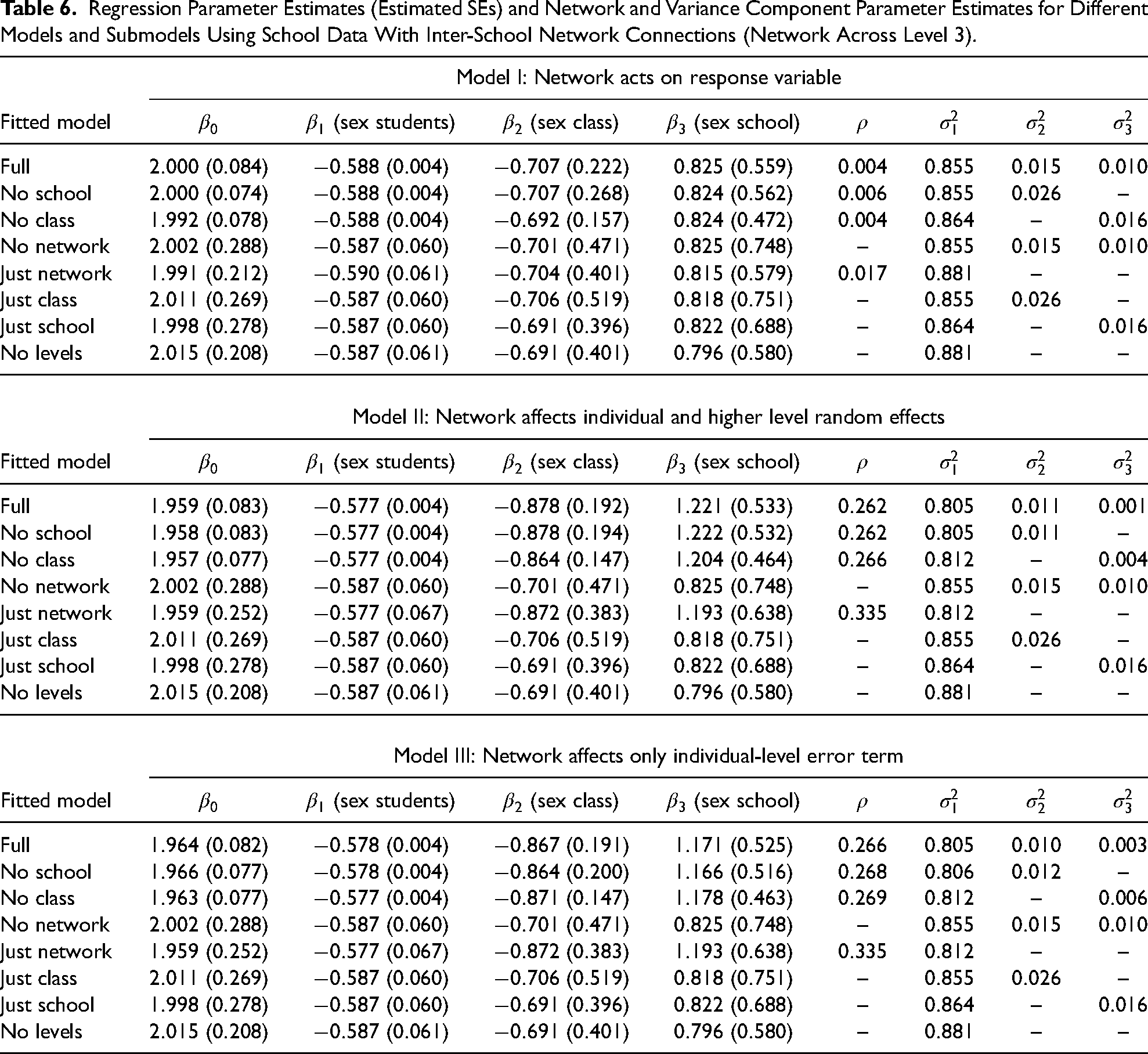
Regression Parameter Estimates (Estimated SEs) and Network and Variance Component Parameter Estimates for Different Models and Submodels Using School Data With Inter-School Network Connections (Network Across Level 3).

	Model I: Network acts on response variable
Fitted model	${\beta }_0$	${\beta }_1$ (sex students)	${\beta }_2$ (sex class)	${\beta }_3$ (sex school)	$\rho$	${\sigma }_1^2$	${\sigma }_2^2$	${\sigma }_3^2$
Full	$2.000$ ( $0.084$ )	$-0.588$ ( $0.004$ )	$-0.707$ ( $0.222$ )	$0.825$ ( $0.559$ )	$0.004$	$0.855$	$0.015$	$0.010$
No school	$2.000$ ( $0.074$ )	$-0.588$ ( $0.004$ )	$-0.707$ ( $0.268$ )	$0.824$ ( $0.562$ )	$0.006$	$0.855$	$0.026$	–
No class	$1.992$ ( $0.078$ )	$-0.588$ ( $0.004$ )	$-0.692$ ( $0.157$ )	$0.824$ ( $0.472$ )	$0.004$	$0.864$	–	$0.016$
No network	$2.002$ ( $0.288$ )	$-0.587$ ( $0.060$ )	$-0.701$ ( $0.471$ )	$0.825$ ( $0.748$ )	–	$0.855$	$0.015$	$0.010$
Just network	$1.991$ ( $0.212$ )	$-0.590$ ( $0.061$ )	$-0.704$ ( $0.401$ )	$0.815$ ( $0.579$ )	$0.017$	$0.881$	–	–
Just class	$2.011$ ( $0.269$ )	$-0.587$ ( $0.060$ )	$-0.706$ ( $0.519$ )	$0.818$ ( $0.751$ )	–	$0.855$	$0.026$	–
Just school	$1.998$ ( $0.278$ )	$-0.587$ ( $0.060$ )	$-0.691$ ( $0.396$ )	$0.822$ ( $0.688$ )	–	$0.864$	–	$0.016$
No levels	$2.015$ ( $0.208$ )	$-0.587$ ( $0.061$ )	$-0.691$ ( $0.401$ )	$0.796$ ( $0.580$ )	–	$0.881$	–	–

	Model II: Network affects individual and higher level random effects
Fitted model	${\beta }_0$	${\beta }_1$ (sex students)	${\beta }_2$ (sex class)	${\beta }_3$ (sex school)	$\rho$	${\sigma }_1^2$	${\sigma }_2^2$	${\sigma }_3^2$
Full	$1.959$ ( $0.083$ )	$-0.577$ ( $0.004$ )	$-0.878$ ( $0.192$ )	$1.221$ ( $0.533$ )	$0.262$	$0.805$	$0.011$	$0.001$
No school	$1.958$ ( $0.083$ )	$-0.577$ ( $0.004$ )	$-0.878$ ( $0.194$ )	$1.222$ ( $0.532$ )	$0.262$	$0.805$	$0.011$	–
No class	$1.957$ ( $0.077$ )	$-0.577$ ( $0.004$ )	$-0.864$ ( $0.147$ )	$1.204$ ( $0.464$ )	$0.266$	$0.812$	–	$0.004$
No network	$2.002$ ( $0.288$ )	$-0.587$ ( $0.060$ )	$-0.701$ ( $0.471$ )	$0.825$ ( $0.748$ )	–	$0.855$	$0.015$	$0.010$
Just network	$1.959$ ( $0.252$ )	$-0.577$ ( $0.067$ )	$-0.872$ ( $0.383$ )	$1.193$ ( $0.638$ )	$0.335$	$0.812$	–	–
Just class	$2.011$ ( $0.269$ )	$-0.587$ ( $0.060$ )	$-0.706$ ( $0.519$ )	$0.818$ ( $0.751$ )	–	$0.855$	$0.026$	–
Just school	$1.998$ ( $0.278$ )	$-0.587$ ( $0.060$ )	$-0.691$ ( $0.396$ )	$0.822$ ( $0.688$ )	–	$0.864$	–	$0.016$
No levels	$2.015$ ( $0.208$ )	$-0.587$ ( $0.061$ )	$-0.691$ ( $0.401$ )	$0.796$ ( $0.580$ )	–	$0.881$	–	–

	Model III: Network affects only individual-level error term
Fitted model	${\beta }_0$	${\beta }_1$ (sex students)	${\beta }_2$ (sex class)	${\beta }_3$ (sex school)	$\rho$	${\sigma }_1^2$	${\sigma }_2^2$	${\sigma }_3^2$
Full	$1.964$ ( $0.082$ )	$-0.578$ ( $0.004$ )	$-0.867$ ( $0.191$ )	$1.171$ ( $0.525$ )	$0.266$	$0.805$	$0.010$	$0.003$
No school	$1.966$ ( $0.077$ )	$-0.578$ ( $0.004$ )	$-0.864$ ( $0.200$ )	$1.166$ ( $0.516$ )	$0.268$	$0.806$	$0.012$	–
No class	$1.963$ ( $0.077$ )	$-0.577$ ( $0.004$ )	$-0.871$ ( $0.147$ )	$1.178$ ( $0.463$ )	$0.269$	$0.812$	–	$0.006$
No network	$2.002$ ( $0.288$ )	$-0.587$ ( $0.060$ )	$-0.701$ ( $0.471$ )	$0.825$ ( $0.748$ )	–	$0.855$	$0.015$	$0.010$
Just network	$1.959$ ( $0.252$ )	$-0.577$ ( $0.067$ )	$-0.872$ ( $0.383$ )	$1.193$ ( $0.638$ )	$0.335$	$0.812$	–	–
Just class	$2.011$ ( $0.269$ )	$-0.587$ ( $0.060$ )	$-0.706$ ( $0.519$ )	$0.818$ ( $0.751$ )	–	$0.855$	$0.026$	–
Just school	$1.998$ ( $0.278$ )	$-0.587$ ( $0.060$ )	$-0.691$ ( $0.396$ )	$0.822$ ( $0.688$ )	–	$0.864$	–	$0.016$
No levels	$2.015$ ( $0.208$ )	$-0.587$ ( $0.061$ )	$-0.691$ ( $0.401$ )	$0.796$ ( $0.580$ )	–	$0.881$	–	–

Example With School Data

School Data Details

For an illustration based on real data, we use a data set about a friendship network and delinquent behavior of students in school classes, collected in a two-wave survey, the Dutch Social Behavior study (Houtzager and Baerveldt 1999). Students from the third and fourth years of the lower middle level of the Dutch secondary school system answered a questionnaire, with a total sample size of 990. A more detailed description can be found at https://www.stats.ox.ac.uk/~snijders/siena/BaerveldtData.html.

The data were collected from 19 schools with two variables of main interest in this article: gender and a measure of delinquent behavior (DB), defined as the number of minor offenses that the respondent states to have committed. The measure was transformed $Y=\ln (1+DB)$ to obtain less skewed data. The network relationship is defined as giving and receiving emotional support: there is a connection from student $i$ to student $j$ if $i$ indicates that $i$ receives and/or gives emotional support from/to student $j$ .

The data only have two levels, schools and students. We artificially added another level, classes, so that we could investigate the effect of ignoring levels in a more complex model with three levels, as we did in Section “Results of Simulation Study.”

The school sizes of the data set are between 31 and 91. We divided the students of each school into classes, such that class sizes are approximately equal and have a maximum size of 31. For example, a school with 31 students was considered to have only one class, but a school with 54 students was split into two classes with 27 students each. The allocation of the students to classes was done randomly until the resulting NAMLM had non-zero estimates of the variance and network parameters.

The response variance $Y$ is the log-transformed delinquent behavior and the student-level covariate is gender. Often covariates are given at several levels. Here we constructed a school- and class-level contextual variable defined as the average gender for schools and classes, respectively, that is, the average rate of males was calculated for each class and each school and were added as covariates (called sex class and sex school).

The network referring to giving and/or receiving emotional support was restricted to within the schools, that is, connections do not exist between any two students of different schools. $\mathbf{W}$ is row-normalized, such that the rows sum to one. The original network has an average of 2.19 links per student. We also artificially created between school connections by adding randomly approximately 0.6 links per student, leading to 2.80 links per student for the new network. The resulting interschool network is denoted by ${\mathbf{W}}_{IS}$ .

Results of Analysis of School Data Using NAMLMs

Effect of omitting levels and networks on estimates of variance components and network parameter

The results for this data set for each of the three NAMLMs are presented in Table 5 (no between school connections) and Table 6 (with between school connections) with the estimates obtained for the full model, containing all three levels and the network, and all submodels obtained by ignoring the network or one or more levels. The tables show the estimates of the regression parameters, their estimated SEs and the estimates of the variance and network parameters. We do not consider the SEs of the variance parameters, because Wald-type confidence intervals are often not applicable and therefore SEs of such variance estimates are of limited use, see Chambers and Chandra (2013) for an alternative bootstrap method to construct confidence intervals.

These results show that when a level, for example, schools or classes, is omitted, then the variance of the omitted level is approximately distributed to the two adjacent levels. For example, when the school level is omitted, then the class-level variance is increased by the variance of the school level. When the class level is omitted, then the variances of the student and school levels are inflated by an amount that sums up to the class-level variance.

The estimate of $\rho$ remains essentially the same provided the school and/or class level is included in the model. When neither level is included, the estimate of $\rho$ increases appreciably as it picks up some of the effects of the omitted levels.

When the network is omitted, then the variances of the levels are all increased for Models II and III. For Model I, there is no or negligible increase, because the network parameter estimate for Model I is very small.

Effect on estimates of regression coefficients

For all three models, the estimates of the regression coefficient for the individual-level covariate do not change as the network or levels are omitted, except for Model I in Table 5 when the network is omitted, consistent with the discussion in Section “Theoretical Impact of Omitting Some Part of the Population Structure in the Analysis.” For the estimates of the regression coefficient of the class-level covariate, ignoring the network has some modest effect in all three models, but ignoring any of the levels has little effect. Similar effects can be seen in the estimates of the regression coefficients for the school-level covariate, although these estimates have quite large estimated SEs due to the small number of schools in the sample.

The observation that ignoring the network affects the estimates of the regression coeffcients for the class and school-level covariates in Models II and III might contradict the discussion in Section “Theoretical Impact of Omitting Some Part of the Population Structure in the Analysis.” However, Tables 5 and 6 show the ML estimates and not OLS estimates, explaining the change of the fixed effects, which is due to the non-zero efficiency effect of the ML estimator, see equation (3) in Berkhof and Kampen (2004). For larger sample size and a larger number of schools and classes, the fixed effects of Models II and III would stay relatively constant, as was seen in the simulation study which involves larger sample sizes. These observations overall confirm the anticipated behavior outlined in Section “Theoretical Impact of Omitting Some Part of the Population Structure in the Analysis.”

Differences between Models I, II, and III

These results also shed some light on the differences and similarities in the results obtained from applying the three different full NAMLMs. For Models II and III, the regression coefficients are the same for the individual-level covariate and very similar for the class and school-level covariates. Comparing results with the naive model that ignores all the dependencies, the individual-level regression coefficients are the same and the estimates for the class, and school covariates tend to be stronger in Models II and III. For Model I, the regression estimates are a little different but still similar to those from Models II and III, and also stronger than those from the naive model. So, for regression coefficients, the models generally give broadly similar estimates, but accounting for the dependencies produces stronger estimates for the higher-level covariates than the estimates obtained from the naive model, although not for the individual-level covariate. This confirms that, especially if higher-level covariates are included, the dependencies should be taken into account, even if not of direct interest. The estimates of the variance components are virtually the same for Models II and III and similar for Model I. When these parameters are of substantive interest, there is little to choose between all three models. The estimate of the network parameter is very similar in Models II and III, but much smaller in Model I. This shows the main difference between Model I and Models II and III. In the latter two, the network dependencies only affect the variance structure, whereas in the former the regression term is also affected, as shown in Section “Extended Models That Include Social Network and Group Dependencies: Network Autoregressive Multilevel Models.” This leads to a smaller network parameter.

Effects on estimated SEs of regression coefficient estimates

Tables 5 and 6 contain the estimated SEs for the estimates of the regression coefficients. It is noticeable that the SEs are smaller when the full model is used, or if only one of the class or school-level effects is omitted. Once simpler variance structures are used, in which any two or more of the network, class, or school effects are omitted, the SEs increase. These increases do not affect the statistical significance of the regression coefficient of the student-level covariate, which stays strongly statistically significant. However, for the class-level covariate, these increases in SEs change the inference from statistically significant to non-significant. The SEs for the school-level regression coefficients are already large because of the small-sample size, and even with the full model are generally non-significant, or sometimes a borderline case, and the increase in SEs leads to strongly non-significant results.

Interpretation of models

Network models and the MLMs both describe dependencies across observations and have been developed in different situations, often influenced by differences in data availability concerning network connections and membership of groups. Using the NAMLMs described in Section “Extended Models That Include Social Network and Group Dependencies: Network Autoregressive Multilevel Models” these two general approaches can be incorporated and interpreted within the same framework. In Section “Network Effects and Network Disturbance Models,” it was noted that autocorrelation in the response variable implicitly introduces a contextual variable determined by the network into the regression part of the model. This is similar to the common and explicit use of contextual variables, such as group means, in MLMs. Examining the variance structures in Section “Re-expressing the Covariance Matrix of NAMLMs,” we can see that the standard MLM can be interpreted in a manner similar to a network model in which each individual is equally connected to all, and only, the individuals within its class or school. The variance component for a level can be converted to an intra-group correlation by dividing by the total of the variance components, and then has a similar interpretation as the network correlation parameter (although in comparing these parameters the fact that the connections due to common group membership are not usually row normalized is relevant). Some of these aspects are discussed by Tranmer and Lazega (2016).

To illustrate the use and interpretation of these models, consider the results for Model II with inter-school connections in Table 6. We will consider submodels with no class effect in the variance structure, as this was artificially generated. In the submodel with network and school (no class sub model), all the regression coefficients are statistically significant and $\hat{\rho }=0.266$ and the intra-group correlation for schools is $\hat{\delta }=0.004$ . When the school level is omitted, so only the network is included, the regression coefficient for class is just statistically significant and the school regression coefficient is not. The network parameter increases to 0.335 as some of the missing within school correlations are picked up by the network effect. When the network is omitted and the school included (just school submodel) the regression coefficients for class and school both are non-significant and the school intra-group correlation increases to 0.016, with some of the omitted network effect also serving to increase the student-level variance from 0.812 to 0.864.

We can compare $\hat{\rho }$ and the intra-school correlation ${\hat{\delta }}_3$ in terms of the correlations between the values of different individuals that they imply. In doing so, we must account for the row normalization of $\mathbf{W}$ used in the analysis. Using the first-order term in the Taylor-series expansion of $\mathbf{A}$ noted in Section “Results From Standard Multilevel Models,” the correlation between the values for individuals $i$ and $j$ arising from the individual-level errors is approximately $\rho (W_{ij}+W_{ji})$ . Due to the row normalization $W_{ij}=n_i^{-1}$ , where $n_i$ is the size of the network centered on individual $i$ . In this example, the average network size is $\approx 2.8$ , and we can use this average value to give an indication of the correlation between two individuals in the network, as $0.266\times 2/2.8=0.19$ , compared with ${\hat{\delta }}_3=0.004$ .

Summary

In this article, we have combined two popular approaches to modeling dependencies across units, such as people, these being network autocorrelation models, and MLMs. This is useful because dependencies arising from a hierarchical structure and network structure may be found together. An example is given in Section “Example With School Data,” where class and school-level random effects are included, as well as a social network reflecting emotional support between students. Depending on assumptions about the components of the MLM that the social network acts upon, three models can be differentiated. In Model I, autocorrelation associated with the network acts directly on the response variable and this leads to the regression component implicitly including a network contextual effect and the variance at each level being affected. In Model II, the network applies to the individual and higher-level random effects, so that the variance at each level is affected, but the regression term is not affected by the network. In Model III, the network applies only to the individual-level random error, so only the variance at the individual level is affected, and the regression term is not affected by the network. These models can be described as NAMLMs. Which of these models is appropriate in a particular situation depends on theoretical and empirical considerations. In practice, we would tend to prefer Model I because it allows network dependencies in both the regression terms, implicitly allowing for a network contextual effect, and the variance components, although we would check diagnostics.

In practice, not all the potential sources of dependencies may be included in an analysis, either because they have not been identified or the data on the network and/or all the group memberships are not available. In some situations, the size of the data set may not be able to support fitting a suitably complex model. Several authors have considered the effect of omitting a level in an MLM on the estimates of the variance components that have been included, and the SEs of the estimates of the regression coefficients. However, there has previously been no consideration of the impact of ignoring a component, either one or more levels and/or the network in the more general framework of NAMLMs. This framework has enabled us to consider these issues analytically, by simulation, and for a real data set. The results show that the expectation of the estimates of the fixed regression coefficients are affected little by omitting the social network or any of the levels. The coefficient of the individual-level covariates is very stable. For Model I, there can be a small effect on the estimates of regression coefficients of the higher-level covariates and the intercept when the network is omitted.

Irrespective of the particular NAMLM used, the results of omitting a component of the variance structure (either the levels of a MLM or the network) are similar. When a level is ignored then the impact on the network parameter (measuring social dependence) generally is minimal, unless the network level is adjacent to or at the omitted level, and usually only the variance parameters of the other, not omitted, levels are affected. Essentially similar rules apply in this case as when ignoring a level in a standard MLM.

Omitting a component of a MLM in a NAMLM has an impact on the variance component estimates, and also on the estimated SEs of the regression coefficients, which may affect the statistical significance of those referring to group-level covariates. Similar conclusions apply as for omitting a level in an MLM (Tranmer and Steel 2001; Berkhof and Kampen 2004; Moerbeek 2004; Van Landeghem, De Fraine, and Van Damme 2005), for example, omitting a level leads to increased variance estimates of the flanking-level variance components and also incorrect estimated SEs of the regression coefficients referring to the omitted (decreased estimated SE) and the flanking levels (often increased estimated SE of the lower flanking level).

However, when the network is omitted then other variance parameters are inflated, depending on how the network and levels interact. Often only the variance parameters of the network level or levels adjacent to the network level are affected.

What happens if several components are omitted at once? When the two levels of the multilevel are ignored, then it seems this also has an effect on the estimation of $\rho$ and not only on the remaining level(s). If the estimated $\rho$ remains constant, then standard MLM results would apply. As we outlined in Section “Theoretical Impact of Omitting Some Part of the Population Structure in the Analysis,” adding a network can be considered as adding other terms in an MLM referring to existing or new level(s). Hence omitting the network, might only affect the same or adjacent levels, for example when the network is at a higher level than the highest level, then only that highest level might be affected. When the network and another level is ignored, then this affects some or all estimated variance parameters. Generally, multiple effects are observed and to avoid incorrect conclusions omitting several components should be avoided, as it is difficult to draw conclusions what would have happened had all levels and the network been accounted for. In general, omitting a component of the variance structure can affect the estimates of those components that are included.

The estimates of the individual-level regression coefficients are robust to omitting components of the variance structure, although there can be some effect on regression coefficients of higher level covariates. The true SEs on the estimates of the regression coefficients were not appreciably affected, but the estimated SEs can be. Even if a full NAMLM cannot be fitted, it is still worthwhile including those components that can be included, and worth bearing in mind that any omitted components may be affecting the estimates of the components that are included in the analysis.

Increases in estimated SEs when levels or the network are omitted reduce the statistical significance of the parameter estimates, leading to some loss of power, but do not lead to incorrectly declaring statistical significance. This was observed in the analysis of the schools data set, which was based on a relatively small sample. In the simulation study, which has a larger sample size, the estimated SEs had negative bias for the regression coefficient of an omitted level. However, this situation is unlikely in practice, since having a covariate for a level usually means we know the level for each individual and can account for it in the variance structure. For the school data set, a reduction in the estimated SEs for a regression coefficient also occurred sometimes, for example, for parameters for covariates for levels adjacent to the omitted level. Hence, for smaller data sets, we need to be careful with declaring significant results for covariates of adjacent levels. Generally, the estimated SEs of the individual-level regression coefficient did not decrease; incorrectly declaring statistically significant results for individual-level covariates is very unlikely to occur when some levels or the network are omitted. Further development of SE estimates for NAMLMs should consider robust SE estimation and bootstrap methods.

The R code produced to fit the NAMLMs is not necessarily made computationally efficient. Furure research could investigate computationally efficient methods to fit these models and also investgate the effects of omitting a level in a MM model to model network and group dependencies proposed by Tranmer, Steel, and Browne (2014) and Tranmer and Lazega (2016), an alternative model approach to the NAMLMs proposed in this article.

Supplemental Material

sj-pdf-1-smr-10.1177_00491241231156972 - Supplemental material for The Effects of Omitting Components in a Multilevel Model With Social Network Effects

Supplemental material, sj-pdf-1-smr-10.1177_00491241231156972 for The Effects of Omitting Components in a Multilevel Model With Social Network Effects by Thomas Suesse, David Steel and Mark Tranmer in Sociological Methods & Research