
Abstract
Large-scale sample surveys are not designed to produce reliable estimates for small areas. Here, small area estimation methods can be applied to estimate population parameters of target variables to detailed geographic scales. Small area estimation for noncontinuous variables is a topic of great interest in the social sciences where such variables can be found. Generalized linear mixed models are widely adopted in the literature. Interestingly, the small area estimation literature shows that multivariate small area estimators, where correlations among outcome variables are taken into account, produce more efficient estimates than do the traditional univariate techniques. In this article, the author evaluate a multivariate small area estimator on the basis of a joint mixed model in which a small area proportion and mean of a continuous variable are estimated simultaneously. Using this method, the author “borrows strength” across response variables. The author carried out a design-based simulation study to evaluate the approach where the indicators object of study are the income and a monetary poverty (binary) indicator. The author found that the multivariate approach produces more efficient small area estimates than does the univariate modeling approach. The method can be extended to a large variety of indicators on the basis of social surveys.
Large-scale sample surveys are usually not designed to produce accurate and precise estimates for small population domains, for example, small geographic areas or small groups in the population (e.g., on the basis of cross-classification between ethnic groups and age bands). However, many social phenomena, such as poverty, well-being, and social exclusion show an important spatial heterogeneity at a small geographic level (Molina and Strzalkowska-Kominiak 2020; Moretti, Shlomo, and Sakshaug 2020; Pratesi 2016). Importantly, policymakers in charge of implementing subnational social policies ask for disaggregated estimates of social indicators. Thus, small area estimates of such phenomena should be produced and released to support decision makers (Pratesi 2016).
In recent years, there has been growing attention to the methodological development of small area estimation methods. Statistical models are now prominent in this field. Indeed, model-based estimators “borrow strength” from related areas using linking models, and they provide more efficient estimates than do direct estimators (see Pfeffermann 2013; Rao and Molina 2015).
The small area estimation approach using linear mixed models is now widely used. These models are powerful given that they include random area effects to take into account between-area variation, that is, the unexplained variability between the small areas. A pioneer work in this context is the Battese, Harter, and Fuller model (Battese, Harter, and Fuller 1988), with further work on mean squared error (MSE) estimation proposed by Prasad and Rao (1990). This model is applicable to continuous response variables, and normality is assumed for the individual error and random area effects. In case of failure of the model assumptions, extensions are proposed in the literature, for example, to account for heteroscedasticity and outliers. Readers may refer to Rao and Molina (2015) for an extensive review of methodological developments.
In the presence of binary outcomes, the generalized linear mixed model (GLMM) with logit link function, that is, a logistic mixed model, is widely adopted. Specifically, an empirical plug-in predictor (EPP) under a GLMM is used in small area estimation of proportions in official statistics (Chandra, Chambers, and Salvati 2012; Chandra, Kumar, and Aditya 2018; Molina and Strzalkowska-Kominiak 2020; Rao and Molina 2015; Salvati, Chandra, and Chambers 2012). For example, the U.K. Office for National Statistics and the Australian Bureau of Statistics use this method (Chambers, Salvati, and Tzavidis 2016; Chandra et al. 2018). Binary variables can be found in most surveys. For instance, some poverty and well-being indicators are based on binary variables (Betti and Lemmi 2013). Additionally, some social indicators estimated on Labour Force Surveys are also constructed on these types of variables (see Chambers et al. 2016; Molina and Strzalkowska-Kominiak 2020). Hence, there is a high demand for small area proportions.
Because many social phenomena are naturally multidimensional (Betti and Lemmi 2013), and therefore correlated, this property can be used to further improve small area estimates (Benavent and Morales 2016; Fabrizi, Ferrante, and Pacei 2005; Moretti et al. 2020; Moretti, Shlomo, and Sakshaug 2021; Ubaidillah et al. 2019). In this context, multivariate small area estimation methods can be applied. Moretti et al. (2020) proposed the use of multivariate small area estimation methods to estimate latent well-being indicators, under the use of the multivariate extension of the Battese, Harter, and Fuller model. This model was studied in detail by Datta, Day, and Basawa (1999). Recently, Moretti (2022) extended a GLMM with logit link function to the case of bivariate proportions, showing good results in terms of efficiency compared with its univariate setting.
In this article, I investigate the multivariate small area estimation problem of continuous and binary response variables jointly. In particular, I apply a joint mixed-modeling strategy to the small area estimation of the mean of a continuous variable and proportion of a binary variable. This is an important problem in sociology and related social sciences. In fact, when building poverty indicators, they can be based on income and measured by a binary indicator taking a value of 0 or 1, denoting whether the personal or household income falls below a poverty threshold (for a review and discussion of poverty indicators, see Pratesi 2016). Therefore, income and poverty indicators are correlated; this can be accounted for in the small area models by assuming a joint modeling strategy.
Notation and Multivariate Small Area Estimation Problem
I now present the notation used in the article and the small area estimation problem we are studying. Let us consider a finite target population
Let
The generic element related to variable
where
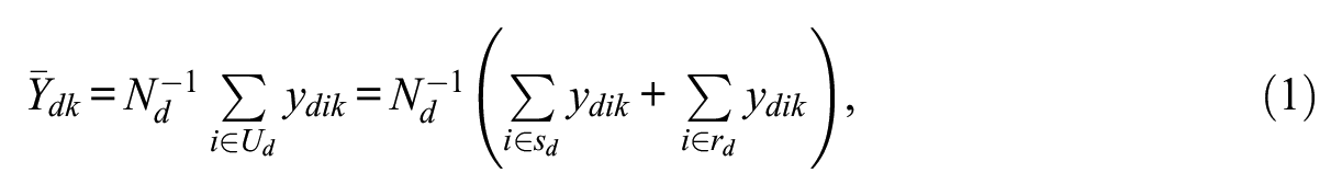
The design-based direct estimator for the kth small area mean
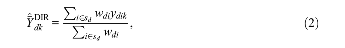
where
It is well known that estimator (2) becomes unstable when
Small Area Estimation under a Joint Mixed Model for Continuous and Binary Outcome Variables
To build indirect small area estimators, statistical models with random area-specific effects that account for between-area variability are used in small area estimation (Rao and Molina 2015). In the univariate small area estimation setting, the Battese, Harter, and Fuller model (Battese et al. 1988) can be used to obtain small area estimates of the population mean in case of continuous variables, that is,
Here, we assume that
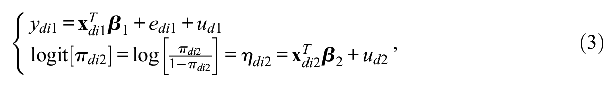
where
Model 3 is a multilevel model for multivariate mixed response types, explaining two outcomes simultaneously (Goldstein 2011), in this case
We assume multivariate (bivariate in this case) normality of the random area effects, that is,

where
Model 3 can be written for
Because of the multivariate nature of the likelihood function, a Gaussian quadrature has been adopted in the literature. ML estimation of the parameters is computationally complex for this model (Berridge and Crouchley 2011; Coull and Agresti 2000). Readers interested in the computations can refer to Appendix A.3 in Berridge and Crouchley (2011). The implementation is fully available in R via the package sabre. 1 This approach is also studied and evaluated in Rabe-Hesketh and Skrondal (2008) and Skrondal and Rabe-Hesketh (2004).
To provide a small area estimator for
Therefore, we can write the EPP of the small area means under model 3 for area
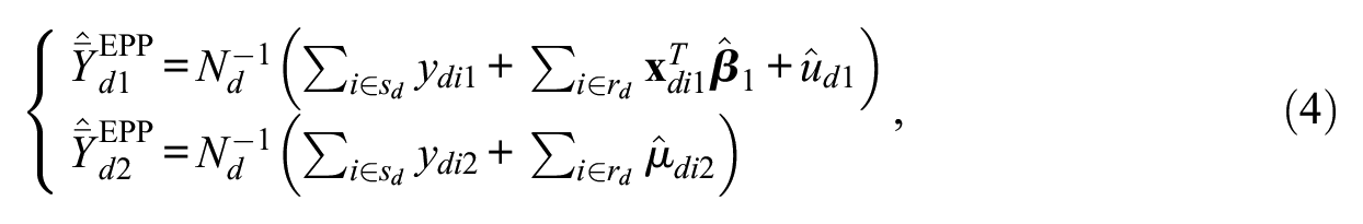
with
In practical applications, the auxiliary variables are available at the unit level for the sample units only, and area-specific aggregates are available for the population from the census or administrative data. As a consequence, equation (4) cannot be applied; however, a modification of it can be derived, and its performance is studied in the literature (Chandra et al. 2018). This is given as follows:
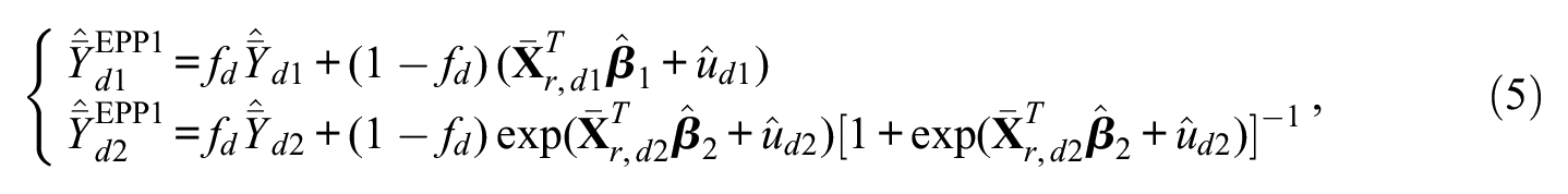
where
When the sampling fractions
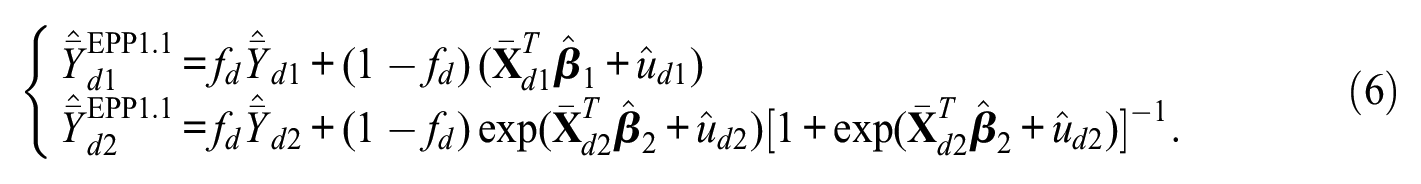
This is reasonable to assume in real data small area applications, given that
MSE Estimation via Parametric Bootstrap
The MSE of equation (6) can be estimated via a parametric bootstrap algorithm. The parametric bootstrap is widely studied and applied in the small area estimation literature, where simulation studies are designed to evaluate the algorithm’s performance (González-Manteiga et al. 2007; Hobza, Morales, and Santamaría 2018; Moretti, Shlomo, and Sakshaug 2020). Here, I extend the algorithm originally developed in González-Manteiga et al. (2007) to the case considered in this article. Note that Moretti et al. (2020) extended and evaluated the algorithm in González-Manteiga et al. (2007) to the bivariate small area estimation of means problem in the case of continuous variables.
The steps of the parametric bootstrap algorithm are as follows:
Estimate model given in equation (3) on the random sample s. The following estimates are obtained:
Generate the bootstrap area-specific random effects as follows:
Calculate the true means of the bootstrap population for variables
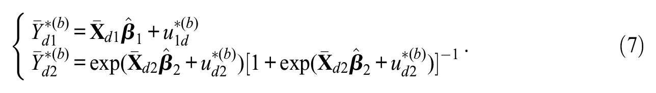
Generate the bootstrap responses
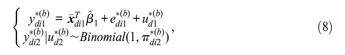
where
Estimate the joint mixed model given in equation (3) on the responses generated at step 4 and obtain the bootstrap EPP1.1 according to equation (6). These are denoted by
Repeat steps 2 to 5
The bootstrap estimators for the MSE of
for
Simulation Study
In this section, I present the results of a design-based simulation study. Design-based simulation studies are important because they allow one to evaluate the performance of the estimators in case of repeated samples drawn from a fixed population that does not exactly follow the assumed model (Molina and Strzalkowska-Kominiak 2020).
Generating the Population
As a fixed target population
The population size in area
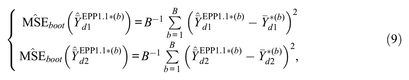
Figure 1 shows the histogram of the logarithmic transformation of income,
Histogram of log income,
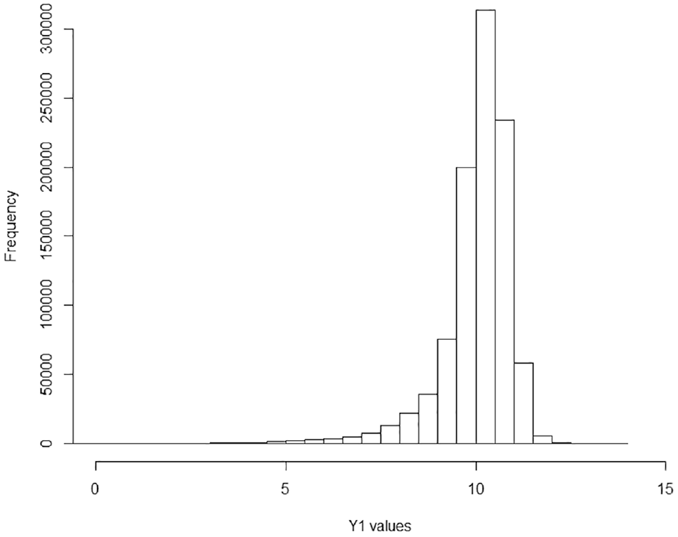
Bar chart of indicator denoting whether the unit’s income is below the poverty line,
Simulation Steps and Quality Measures
The simulation consists of the following steps, where
From the target population
Estimate the joint mixed model given in equation (3) and the univariate mixed models on each separate response in each sample
The following measures of performance are calculated to evaluate the estimators for
Absolute relative bias (ARB)

Root MSE (RMSE)
Relative root MSE (RRMSE)

where
% Relative reduction in terms of RMSE (RelRed%)

To present summary statistics, the median across the small areas
Results
I now present the results of the simulation study with a focus on the quality measures presented above. Table 1 shows the median across the small areas of the ARB and RRMSE of the estimates obtained via the direct, univariate, and multivariate estimators for
Median Values across Small Areas of ARB and RRMSE of the Estimates Obtained via the Direct, Univariate, and Multivariate Estimators for
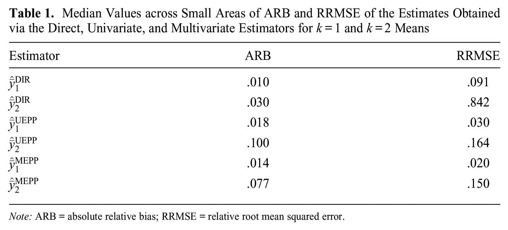
Note: ARB = absolute relative bias; RRMSE = relative root mean squared error.
As shown, the ARB is small (negligible) across all the estimators. The multivariate approach produces estimates with a smaller ARB compared with the univariate case. Thus, it does not introduce much bias in the small area estimates. Furthermore, the multivariate small area predictor provides estimates with a smaller RRMSE compared with the univariate and direct estimators. Hence, the multivariate approach returns more efficient estimates compared with the univariate approach. This latter point can be seen if we consider the percentage relative reductions in terms of RMSE. Indeed, these are satisfactory and equal to
Figures 3 and 4 plot the RRMSE across the small areas where we compare the RRMSE of the multivariate versus univariate approach and their direct estimators setting for
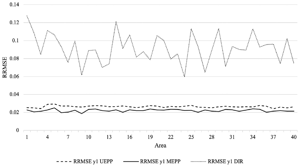
Relative root mean squared error (RRMSE) of small area estimates for direct (DIR; dotted line), univariate (UEPP; dashed line), and multivariate (MEPP; solid line) estimators for the mean of log income, k = 1, ordered by decreasing sampling fraction.
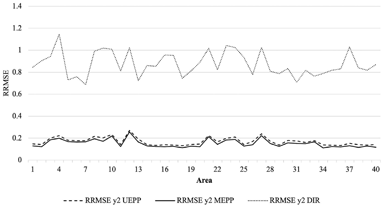
Relative root mean squared error (RRMSE) of small area estimates for direct (DIR; dotted line), univariate (UEPP; dashed line), and multivariate (MEPP; continuous line) estimators for the poverty proportion, k = 2, ordered by decreasing sampling fraction.
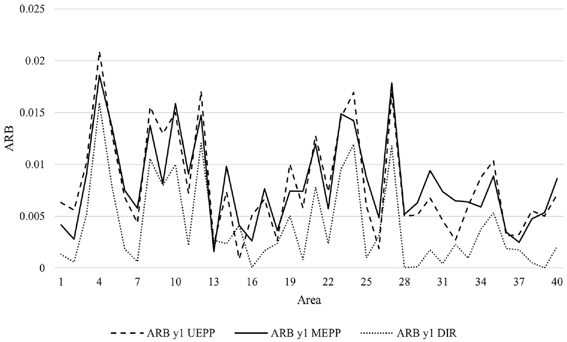
Absolute relative bias (ARB) of small area estimates for direct (DIR; dotted line), univariate (UEPP; dashed line), and multivariate (MEPP; solid line) estimators for the mean of log income, k = 1, ordered by decreasing sampling fraction.
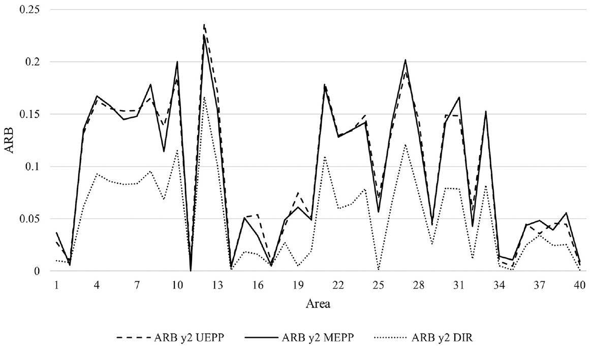
Absolute relative bias (ARB) of small area estimates for direct (DIR; dotted line), univariate (UEPP; dashed line), and multivariate (MEPP; solid line) estimators for the poverty proportion, k = 2, ordered by decreasing sampling fraction.
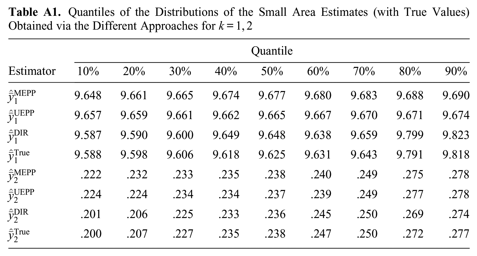
As expected, Figures 3 to 6 demonstrate that the direct estimates suffer from a large RRMSE but very small ARB across all the small areas. The multivariate approach provides estimates with a smaller RRMSE than both the univariate and direct approaches, which is in line with the multivariate small area estimation literature. In addition, the ARB of the multivariate estimates is negligible across all the areas, showing it does not introduce a large bias in the estimates. I did not find any relationship between the sampling fraction and performances of the multivariate approach over its univariate setting. Figures A1 and A2 and Table A1 in Appendix A provides additional simulation outputs that are helpful for interpreting the results.
In summary, the results of this simulation study are promising. Although the income variable,
Conclusion and Future Research Directions
In this article, I studied the multivariate small area estimation problem in the case of mixed-type variables. The multivariate small area estimation literature has paid particular attention to the case of continuous variables. However, noncontinuous variables are widely diffused in social surveys. In this work, I considered the unit-level small area estimation approach, assuming the auxiliary variables are known for all the sampled units. I did not investigate the area-level approach in the present article. For the area-level approach, the reader may refer to Fay (1987), and more recent studies by Benavent and Morales (2016, 2020).
I compared a multivariate EPP with its univariate setting, where two mixed models are estimated separately on each response variable in a design-based simulation study. The predictors based on the univariate setting are used by different statistical agencies due to their good properties. I found the multivariate approach provides more reliable small area estimates than does the univariate approach. In particular, the multivariate predictor produces small area estimates with a smaller RRMSE, as well as bias slightly smaller than the univariate approach. Larger gains in efficiency can be seen for the continuous case.
The modeling strategy evaluated in this article is flexible, because joint mixed models can account for variables measured on different scales at the same time. Thus, we can improve the efficiency of the small area estimates by “borrowing strength” across response variables in a model-based, small area estimation approach.
These types of variables are widely present in social surveys, where continuous variables are strongly related to binary variables. Here, I considered income and poverty indicators; however, future work will investigate other modeling scenarios, that is, variables measured on other scales, such as models for count data. Indeed, the use of multivariate mixed (multilevel) models is of particular relevance in sociology, where multivariate research questions can be formulated and answered by interpreting model parameter estimates, in particular the association parameters. These association parameters, such as correlations, can be estimated via the use of multivariate models. For example, the literature has shown a strong relationship between happiness and health (see Argyle 1997; Graham 2012). If one considers a continuous latent variable measuring happiness, and a binary variable measuring a health domain, the model object of this study can be applied to investigate relationships in the case of multilevel data. Pierewan and Tampubolon (2015) used a multivariate mixed model to investigate the relationships between happiness and health. The model I proposed in this small area estimation problem can be used to investigate subnational differences of such indicators, and to produce more efficient estimates than in the scenario where two separate multilevel models are estimated.
In the context of income and expenditures analysis, researchers might be interested in studying relationships between deprivation and expenditures; these show correlations (see Moretti and Shlomo 2023) that can be taken into account in the modeling stage. Income is also related to food poverty. Thus, a binary variable indicating whether a household is food deprived or at risk for food deprivation can be built, and this is strongly related to household income (for the link between poverty and food insecurity, see Wight et al. 2014). Therefore, similar to the approach followed in the simulation study, the method proposed here is appropriate to provide geographic understanding around food deprivation and monetary poverty dimensions.
It is important to acknowledge that the mixed models adopted in this article can be extended to a spatial dependence setting (Chandra, Chambers, and Salvati 2019; Chandra et al. 2018). Here, one strategy to incorporate spatial information into the models is to extend the random effects model allowing for spatially correlated random area effects. For instance, this can be achieved by using a simultaneous autoregressive model (Anselin 1988; Cressie 2015). As highlighted by Chandra et al. (2018), in practical applications, it is often reasonable to consider that the effects of neighboring geographic areas are correlated (defined by a contiguity matrix that is included in the modeling stage). Readers interested in simultaneous autoregressive models in small area estimation can refer to the following literature, which presents extended evaluations and applications: Singh, Shukla, and Kundu (2005), Pratesi and Salvati (2008), Pratesi and Salvati (2009), Molina (2009), Marhuenda, Molina, and Morales (2013), and Porter, Wikle, and Holan (2015). In addition, Bayesian approaches to small area estimation considering conditionally autoregressive models can model the spatial dependence (see Besag, York, and Mollié 1991; Leroux, Lei, and Breslow 2000; Mercer et al. 2014). These spatial extensions are widely used for small area estimation problems of health and social indicators in sociology, demography, and epidemiology. Dwyer-Lindgren et al. (2016) used the spatial Besag-York-Mollie model (Besag et al. 1991) to estimate mortality rates. The Centers for Disease Control and Prevention PLACES project adopted a similar strategy to estimate small area indicators of morbidity (https://www.cdc.gov/places/methodology/index.html). Regarding poverty indicators, readers may refer to Marhuenda et al. (2013) and Giusti, Masserini, and Pratesi (2017). In this article, I did not include a spatial process into the random area effects. Spatial extensions of the proposed methods are interesting and useful for users, and they will be the subject of future research given they require particular methodological attention.
Footnotes
Appendix A: Extra Outputs of the Simulation Study
Quantiles of the Distributions of the Small Area Estimates (with True Values) Obtained via the Different Approaches for
| Estimator | Quantile | ||||||||
|---|---|---|---|---|---|---|---|---|---|
| 10% | 20% | 30% | 40% | 50% | 60% | 70% | 80% | 90% | |
| 9.648 | 9.661 | 9.665 | 9.674 | 9.677 | 9.680 | 9.683 | 9.688 | 9.690 | |
| 9.657 | 9.659 | 9.661 | 9.662 | 9.665 | 9.667 | 9.670 | 9.671 | 9.674 | |
| 9.587 | 9.590 | 9.600 | 9.649 | 9.648 | 9.638 | 9.659 | 9.799 | 9.823 | |
| 9.588 | 9.598 | 9.606 | 9.618 | 9.625 | 9.631 | 9.643 | 9.791 | 9.818 | |
| .222 | .232 | .233 | .235 | .238 | .240 | .249 | .275 | .278 | |
| .224 | .224 | .234 | .234 | .237 | .239 | .249 | .277 | .278 | |
| .201 | .206 | .225 | .233 | .236 | .245 | .250 | .269 | .274 | |
| .200 | .207 | .227 | .235 | .238 | .247 | .250 | .272 | .277 | |
Appendix B: R Program
This R program can be used to apply the methods used in this article. First, to estimate multivariate mixed models, such as the joint mixed model introduced in the article, the software sabre can be installed from http://sabre.lancs.ac.uk/installing_intro.html and then installed in R manually.
A possible R program that can be used to replicate the results of the simulation study for the multivariate case is given below. An R program for the univariate case is available in Chandra et al. (2018).