The Statistical Advantages of Multilevel Analysis of Individual Heterogeneity and Discriminatory Accuracy for Estimating Intersectional Inequalities

Abstract

Multilevel Analysis of Individual Heterogeneity and Discriminatory Accuracy (MAIHDA) is a multilevel regression approach grounded in intersectionality theory. It examines inequalities across intersections of social identities (e.g., gender, ethnicity, class) and is argued to provide more accurate predictions of intersectional means than conventional methods that estimate group means directly or via regressions with all interactions. This study evaluates that claim using analytic expressions and an empirical illustration to compare simple and MAIHDA-predicted means against population values. Predictive accuracy is assessed via variance, correlation, bias, and mean squared error. Results show that MAIHDA estimates generally outperform simple means, particularly when decomposing intersectional means into additive and non-additive identity effects. The magnitude of the advantage depends on inequality patterns and group sample sizes. MAIHDA is especially valuable when inequalities are subtle or data for marginalized intersections are sparse—conditions common in practice. These findings highlight MAIHDA's practical relevance for quantitative intersectionality research.

Introduction

Multilevel analysis of individual heterogeneity and discriminatory accuracy (MAIHDA) is a recently developed multilevel regression modeling approach designed to explore complex social inequalities in individual outcomes (Evans et al. 2018). MAIHDA is motivated by intersectionality theory (Collins and Bilge 2020; Crenshaw 1989), which observes that individuals’ lived experiences and outcomes are shaped by their positionalities within complex and interlocking systems of oppression, including sexism, racism, and socioeconomic inequality. MAIHDA quantifies inequalities across intersections of multiple social identities and positionalities (e.g., gender, ethnicity, and social class), rather than focusing on one axis of inequality at a time. The growing adoption of MAIHDA reflects widespread interest in quantitative methods that align with intersectionality's demands for expansive consideration of diversity (Bauer et al. 2021; McCall 2005; Merlo 2018).

While early applications were primarily in social epidemiology, MAIHDA is increasingly being used across the social sciences, with applications in criminology (Pina-Sánchez and Tura 2024; Tura et al. 2024), education (Giaconi et al. 2024; Keller et al. 2023; Prior et al. 2022; Prior and Leckie 2024; Van Dusen et al. 2024), environmental justice (Alvarez et al. 2022), gender studies (Ivert et al. 2020; Silva and Evans 2020), organizational studies (Humbert 2024), psychiatry (Forrest et al. 2023), and social work (Lister, Hewitt and Dickerson 2024; Pomeroy and Fiori 2025). For example, Keller et al. (2023)—an application we will return to later—applied MAIHDA to study intersectional inequalities in 15-year-old students’ reading scores across four social identities: Gender, immigrant status, parental education, and parental occupational status.

Evans et al. (2024a) present an introduction and tutorial on MAIHDA for those completely new to the approach. Here, we summarize the key points. MAIHDA was developed in response to perceived weaknesses of the conventional approach to studying intersectionality, which typically involves estimating linear regression models on social identities (Evans et al. 2018). These weaknesses include the assumption that the effects of social identities are additive, which may overlook how systems of oppression interact in more complex, multiplicative ways. When interaction terms are considered, often just a single two-way interaction is included. Including all possible interactions, however, quickly leads to many regression coefficients, resulting in overfitting and challenges with interpretation. Interpretation, if not overfitting, is eased by predicting and comparing the mean outcome for each intersectional group. We refer to these as simple means as they are equal to the arithmetic means obtained by calculating the mean separately for each group.

The MAIHDA approach, in contrast, is grounded in the multilevel modeling framework (Raudenbush and Bryk 2002; Snijders and Bosker 2012). It involves fitting a sequence of two multilevel regression models where individuals (level 1) are nested in intersectional social strata (level 2), henceforth referred to as intersections. Thus, Intersection 1 might refer to native female students with low parental education and low parental occupation. Intersection 2 might then be native female students with low parental education and low-to-middle parental occupation, and so on. For simplicity, we focus on MAIHDA models for continuous outcomes, though MAIHDA models can be applied to all outcome types.

The first multilevel model, henceforth referred to as MAIHDA Model 1, is a two-level model without any covariates. The model estimates the overall magnitude of intersectional inequalities in the data and predicts the mean outcome for each intersection. This facilitates the identification of social identity combinations associated with the most and least favorable mean outcomes.

The second multilevel model, henceforth referred to as MAIHDA Model 2, is a two-level model in which the social identity variables used to construct the intersections are included as main-effect covariates. The model examines the extent to which intersectional inequalities deviate from the simplest additive patterns of social identities—for example, whether the gender-based mean outcome difference remains constant across different values of immigrant status, parental education, and parental occupational status. By assessing these deviations, Model 2 can reveal hidden social processes that emerge only for specific social identity combinations, as well as quantify consistent or typical patterns (e.g., women tend to experience worse outcomes than men).

A central argument made by proponents of MAIHDA is that its intersectional means provide more accurate predictions of the population means than do simple means (Evans et al. 2018; Evans et al. 2024b). This claim is based on earlier findings from the statistical literature on multilevel models (Raudenbush and Bryk 2002; Snijders and Bosker 2012). However, these findings and their implications are less well understood by applied researchers, especially, within the context of MAIHDA. Fundamentally, how much more accurate are MAIHDA means than simple means? What does their relative accuracy depend on, and how does this vary across a wide range of possible scenarios? Most importantly, is the choice between simple and MAIHDA means likely to affect conclusions in real-world research? These questions and their answers matter. If the community of intersectional researchers using MAIHDA unknowingly make incorrect choices—leading to results that would have differed if a preferred approach had been used—then they risk mischaracterizing inequalities, inefficiently targeting marginalized groups, and misallocating resources, all of which can have harmful consequences for individuals and society.

The arguments in favor of MAIHDA predicted means over simple means are typically based on two key points from the multilevel literature. First, simple means exhibit high sampling variability when the number of individuals per intersection is low. Second, MAIHDA means address this issue as they are defined as conditional expectations of the population given the data, which shrink their predictions from the simple means toward model-implied means—that is, the means predicted by the intercept and the main effect covariates if included) (Raudenbush and Bryk 2002; Snijders and Bosker 2012). Greater shrinkage is applied to the smallest intersections. Shrinkage is viewed as beneficial because it protects against overinterpreting extreme predictions that may have arisen due to chance (sampling variation). When the models are estimated by frequentist methods (maximum likelihood (MLE) or restricted maximum likelihood (REML)) these expectations are calculated using empirical Bayes prediction. When Bayesian methods (Markov chain Monte Carlo—MCMC) are used, the posterior distributions of the intersection means are estimated and are then summarized by their posterior means.

Importantly, the means predicted by MAIHDA Model 1 and Model 2 also differ from one another. This variation stems from the difference in their model-implied means—or, in other words, the values toward which the predictions are shrunk. In Model 1, the model-implied means are simply the overall or grand mean, so final predictions are shrunk toward this single value. Thus, the final predictions are informed by both the data from that intersection and the overall data. This shrinkage is therefore sometimes referred to as partial pooling. In Model 2, the model-implied means are the means implied by the estimated additive effects of the social identities used to define the intersections. The predictions in Model 2 are therefore shrunk toward these intersection-specific values. To the extent that the MAIHDA-predicted means are preferable to the simple means, the Model 2 means are expected to be preferable to the Model 1 means, as they will lie closer to the true population means for each intersection.

Several simulation studies have started to examine the predictive accuracy of the MAIHDA means. Bell, Holman and Jones (2019) simulated data from linear regression models, primarily without interaction terms, and compared Type I error rates among simple means, MAIHDA Model 1, and Model 2 means. Their findings suggest that MAIHDA Model 2 means result in a lower Type I error rate than both Model 1 and simple means.

Mahendran, Lizotte and Bauer (2022a, 2022b) expanded on this by simulating data from linear and logistic regression models with various interaction terms. They compared MAIHDA Model 2 means to simple means. For both continuous and binary outcomes, they concluded that MAIHDA Model 2 means offer greater accuracy than simple means, particularly for smaller intersection sizes.

Van Dusen et al. (2024) simulated data from MAIHDA Model 2 and found that Model 2 means outperform simple means, with the performance gap widening as intersection sizes decrease.

While these studies consistently show that MAIHDA Model 2 means outperform simple means, they provide little insight into why this occurs, beyond broadly attributing it to shrinkage. They also offer minimal exploration of MAIHDA Model 1 means and do not examine how the relative merits of all three means might vary based on the nature of the intersectional inequalities being studied.

In this study, we aim to evaluate—and clearly demonstrate to the community of quantitative intersectionality researchers—the claim that MAIHDA means are more accurate than simple means. We seek to explain when and why these different means diverge and to provide guidance on which to report in practice. Specifically, we present and analyze analytical expressions that describe how these means vary across intersections relative to the true variance, and how they correlate with the true intersection means. We then assess the statistical properties of each approach for a given intersection of interest, deriving and analyzing expressions for the bias, variance, and mean squared error (MSE) of the three means based on random samples of individuals within that intersection. While these expressions are not themselves new—since MAIHDA models are multilevel models—their interpretation in the context of MAIHDA, and thus their relevance to intersectional research, is novel. Across both sets of analyses, we examine how these properties vary as a function of the overall magnitude of intersectional inequalities, the extent to which those inequalities follow an additive pattern, and key data characteristics, including the mean and variability of intersection sizes.

The Two Maihda Models

In this section, we provide a brief review of the two MAIHDA models.

Model 1: Empty, Null, or Unadjusted Model

Model 1 is a two-level model without any covariates. Let $y_{ij}$ denote the outcome for individual i ( $i=1,\dots ,n_j$ ) at intersection j ( $j=1,\dots ,J$ ). The model can then be written as:

$$y_{ij}={\mu }_j+e_{ij}$$

(1)

where ${\mu }_j$ denotes the population or true mean outcome at intersection $j$ —that is, the mean outcome if the entire population of individuals at that intersection were observed, rather than just a sample. The term $e_{ij}$ is an individual residual measuring how each individual's outcome deviates from the true mean for their intersection. The true mean is then specified as:

$${\mu }_j={\beta }_0+u_j$$

(2)

where ${\beta }_0$ is fixed-effect intercept measuring the overall mean or grand mean across all intersections, and $u_j$ is a random effect measuring how each intersection's true mean deviates from the overall mean. Substituting (2) into (1) and rearranging gives the combined equation:

$$y_{ij}={\beta }_0+u_j+e_{ij}$$

(3)

The intersection random effects and individual residuals are each assumed normally distributed with constant variances ${\sigma }_u^2$ and ${\sigma }_e^2$ . Thus, ${\sigma }_u^2$ is also the variance of the true means about the overall mean.

The overall magnitude of intersectional inequalities is measured by the variance partition coefficient (VPC), which quantifies the proportion of outcome variance that lies between the intersection means:

$$\mathrm{VPC}={\displaystyle \frac{{\sigma }_u^2}{{\sigma }_u^2+{\sigma }_e^2}.}$$

(4)

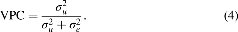
The VPC can range from 0 to 1, with higher values indicating greater intersectional inequalities. Most applications find VPCs ranging from 0.01 to 0.20, suggesting that the studied social stratifications account for 1–20% of the outcome variation (Evans et al. 2024a). Conversely, 80–99% of the variation reflects other unmodeled individual characteristics.

When the models are estimated using frequentist methods (MLE or REML), empirical Bayes prediction is applied post-estimation to assign values to the random effects $u_j$ , which are then used to predict the intersection means ${\mu }_j$ . In contrast, Bayesian methods (MCMC) estimate the posterior distributions of the intersection means simultaneously with the model parameters, typically summarizing them by their posterior means. Analyzing these intersection means enables the identification of social identity combinations linked to the most and least favorable outcomes. Henceforth, for simplicity, we refer to predicting the intersection means, without distinguishing between prediction and estimation as defined under frequentist or Bayesian frameworks.

Model 2: Full, Main Effects, or Adjusted Model

Model 2 is a two-level model in which the social identity variables used to construct the intersections are included as main-effect covariates. The model can be written as:

$$y_{ij}={\mu }_j+e_{ij}$$

(5)

$${\mu }_j={\beta }_0+{\beta }_1{x}_{1j}+\cdots +{\beta }_p{x}_{pj}+u_j$$

(6)

where $x_{1j},\dots ,x_{pj}$ denotes the social identity variables (entered as dummy variable covariates) used to define the intersections, ${\beta }_1,\dots ,{\beta }_p$ are the associated fixed-effect regression coefficients capturing the additive patterns in the intersection inequalities. The term $u_j$ is the intersection random effect, measuring how each intersection's true mean deviates from that implied by the additive effects; in other words, it captures all two-way and higher-order interaction variability. Thus, ${\sigma }_u^2$ now measures the variance associated with this non-additivity.

Substituting (6) into (5) gives the combined equation:

$$y_{ij}={\beta }_0+{\beta }_1{x}_{1j}+\cdots +{\beta }_p{x}_{pj}+u_j+e_{ij}$$

(7)

The extent to which the intersectional inequalities are additively patterned is assessed via the proportion change in variance (PCV) statistic. The PCV measures the reduction in intersection variance when moving from Model 1 to Model 2. This is given by:

$$\mathrm{PCV}={\displaystyle \frac{{\sigma }_{u1}^2-{\sigma }_{u2}^2}{{\sigma }_{u1}^2}}$$

(8)

where the $1$ and $2$ subscripts distinguish between the Model 1 and Model 2 intersection random effect variances. Thus, $1-\mathrm{PCV}$ measures the degree to which intersectional inequalities deviate from those implied by additivity and, therefore, the extent to which hidden social processes may be at play, occurring only for certain social identity combinations. Put differently, the PCV accounts for how much of the overall inequality quantified by Model 1 follows a consistent pattern (e.g., female students consistently score higher than male students, regardless of other characteristics), while $1-\mathrm{PCV}$ accounts for departures from this pattern (e.g., gender inequality is larger among immigrants).

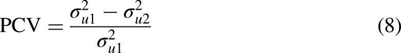
The PCV can range from 0 to 1, with higher values indicating a greater additive structure. When the PCV equals 0, there is no additive structure at all, and Model 2 simplifies to Model 1. However, in practice, we typically see a PCV that suggests a mix of additive (consistent) and interaction (unique departures) inequality patterns. Most empirical applications find PCVs ranging from 0.60 to 0.95, suggesting that 60–95% of the variation in mean outcomes across intersections follows an additive pattern (Evans et al. 2024a). Conversely, 5–40% of the variation reflects more complex interaction effects.

The individual residual variance $e_{ij}$ , in contrast, does not change when moving from Model 1 to Model 2, as the social identities are intersection-level covariates and therefore do not explain outcome heterogeneity within intersections.

As with Model 1, we can predict the intersection means ${\mu }_j$ . Additionally, we can decompose each predicted mean outcome into its additive and non-additive effect, allowing identification of specific intersections where non-additivity occurs. To do this, a 95% confidence interval (for frequentist estimation) or a 95% credible interval (for Bayesian estimation) is typically constructed around the non-additive effect $u_j$ to determine which intersections significantly deviate from what would be expected under an additive model. However, we do not explore this further here.

Illustrative Application

Keller et al. (2023) presented the first application of MAIHDA in educational research. They applied MAIHDA to 5451 student reading performance scores from the German sample of the Program for International Student Assessment (PISA) 2018. They considered four social identities: gender (male, female), immigrant status (native, immigrant), parental education (low, high, as measured by university entrance certificate), and parental occupational status (low, low-middle, middle, middle-high, high). Combining these categories resulted in 40 intersections $(=2\times 2\times 2\times 5$ ). Their descriptive statistics showed that the mean and standard deviation (SD) of reading performance were 498 and 106, respectively (versus the OECD average mean and SD of 485 and 105). Female students scored higher than male students, native students outperformed immigrant students, students whose parents held a university entrance certificate scored higher than those whose parents did not, and students from families with higher occupational status achieved higher scores (see their Table 1).

Table 1.

Results of MAIHDA Models 1 and 2 for reading achievement in the Keller et al. (2023) study.

	Model 1		Model 2
	Est.	SE	Est.	SE
Intercept	478.3	[464.3, 492.3]	468.4	[452.8, 483.3]
Gender
Female (Ref.)			−
Male			−25.6	[-36.5, -14.9]
Immigrant background
Native (Ref.)			−
Immigrant			−42.5	[-53.7, -30.9]
Highest parental education
Below uni. entrance certificate (Ref.)			−
At least uni. entrance certificate			29.8	[18.2, 42.0]
Highest parental occupation status
Low (Ref.)			−
Low to middle			10.1	[-5.9, 26.8]
Middle			27.6	[11.4, 44.6]
Middle to high			53.1	[35.2, 70.4]
High			62.6	[40.5, 81.2]
Intersection variance	1698.3		144.4
Student variance	9011.7		9021.2
VPC	15.9%		1.6%
PCV	−		91.2%

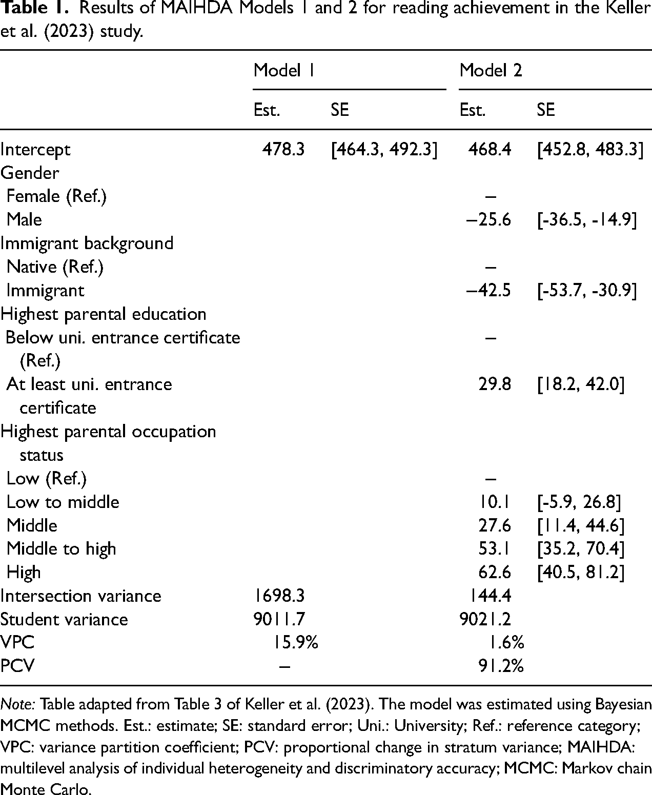
Note: Table adapted from Table 3 of Keller et al. (2023). The model was estimated using Bayesian MCMC methods. Est.: estimate; SE: standard error; Uni.: University; Ref.: reference category; VPC: variance partition coefficient; PCV: proportional change in stratum variance; MAIHDA: multilevel analysis of individual heterogeneity and discriminatory accuracy; MCMC: Markov chain Monte Carlo.

Table 1 presents their results from MAIHDA Model 1 and Model 2 estimated using Bayesian MCMC methods (see their Table 3). The Model 1 VPC statistic reveals substantial intersectional inequalities: 16% of the variance in student achievement lies between the intersection means. The Model 2 regression coefficients estimate the additive structure in the intersectional means, and these results align with their descriptive statistics. The PCV statistic shows that the additive structure accounts for 91% of the variation in the intersection means, meaning that 9% of the variation reflects deviations—both positive and negative—from the model-implied additive patterns of inequality. In other words, variation associated with two-way and higher-order interactions captured by the intersection random effect. Indeed, six of their intersection means deviate by 10 or more points from additivity (approximately 0.1 SD or more), but only one of these departures is statistically significant (see their Figure 4). Intersection 40, Female, native students with university entrance certificate parents and high occupational status—already the highest-scoring intersection in terms of additive effects—scored around 15 points higher (0.15 SD) than what additivity would suggest.

Figure 1 shows the simple means and the MAIHDA Model 1 and Model 2 means for all 40 intersections, and where we have highlighted the six intersections with 20 or fewer individuals. For most intersections, the means are very similar across the three methods. However, as expected, the means for smaller intersections (highlighted) notably vary across methods (see also Table 2). Specifically, compared to the simple means, the MAIHDA Model 1 means are shrunk toward the overall average. Relative to the MAIHDA Model 1 means, the MAIHDA Model 2 means generally increase, except for Intersection 35, which decreases. In the most extreme case, Intersection 39 (male, immigrant, low parental education, high occupational status; n = 3), the three means are 362, 438, and 458, with a range of 96 points (approximately 0.96 SD). These results clearly demonstrate that the different prediction methods can yield substantively different results, especially when intersection sizes are small.

Figure 1.

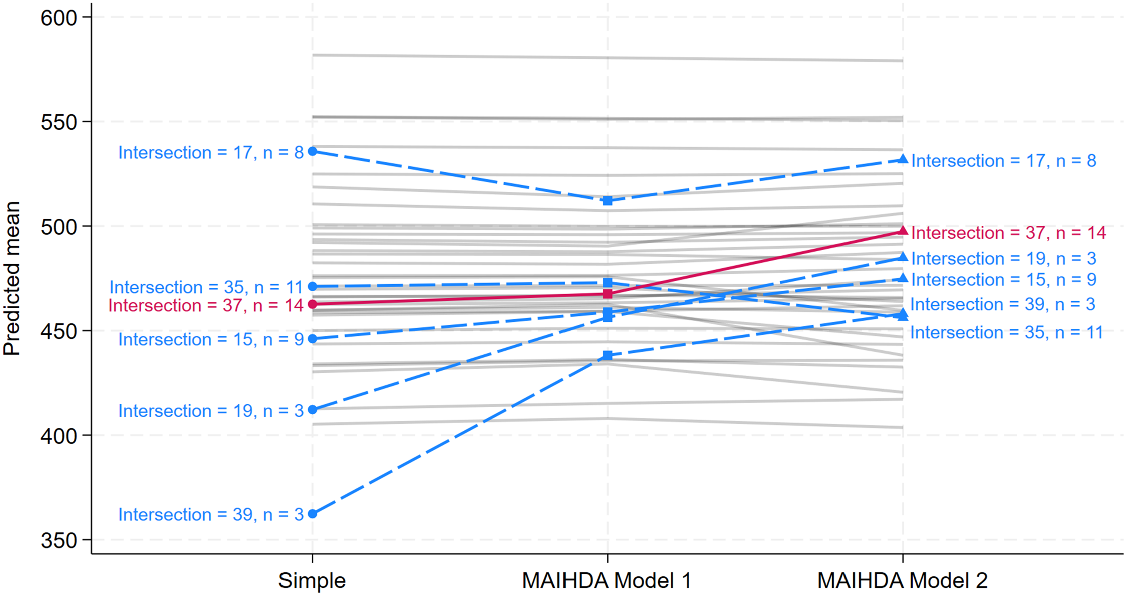
Predicted simple means, multilevel analysis of individual heterogeneity and discriminatory accuracy (MAIHDA) model 1 means, and MAIHDA model 2 means for all 40 intersections in the Keller et al. (2023) study. The six intersections with fewer than n = 20 individuals are emphasized both in the plot and in Table 2. Additionally, Intersection 37 is highlighted in the plot, as it is examined in more detail in Figure 2. The simple means are defined in (9), the MAIHDA Model 1 means in (10), and the MAIHDA Model 2 means in (14).

Table 2.

Predicted intersection means for the six intersections with fewer than $n$  = 20 individuals in the Keller et al. (2023) study.

							MAIHDA Model 1			MAIHDA Model 2
ID					Size	Simplemean	Rel.	Modelimplied mean	MAIHDA mean	Rel.	Modelimplied mean	MAIHDA mean
$j$	Gender	Migrant	Education	Occupation	$n_j$	${\overline{y}}_{.j}$	$R_j$	${\beta }_{0,1}$	${\tilde{\mu }}_j$	$R_j$	${\mathbf{x}}_j^{\mathrm{\prime }}{\beta }_2$	${\tilde{\mu }}_j$
15	Female	Immigrant	Below UEC	Mid to high	9	446	0.63	478	459	0.13	479	475
17	Female	Native	Below UEC	High	8	536	0.60	478	512	0.11	531	532
19	Female	Immigrant	Below UEC	High	3	412	0.36	478	456	0.05	489	485
35	Male	Immigrant	Below UEC	Mid to high	11	471	0.67	478	473	0.15	453	456
37	Male	Native	Below UEC	High	14	463	0.73	478	468	0.18	505	497
39	Male	Immigrant	Below UEC	High	3	362	0.36	478	438	0.05	463	458

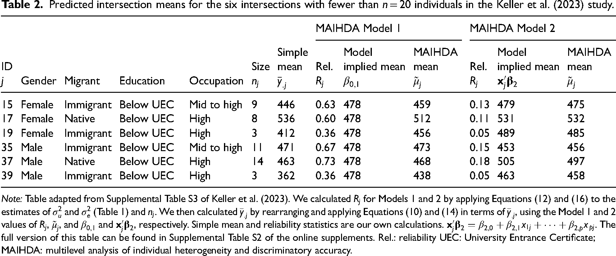
Note: Table adapted from Supplemental Table S3 of Keller et al. (2023). We calculated $R_j$ for Models 1 and 2 by applying Equations (12) and (16) to the estimates of ${\sigma }_u^2$ and ${\sigma }_e^2$ (Table 1) and $n_j$ . We then calculated ${\overline{y}}_{.j}$ by rearranging and applying Equations (10) and (14) in terms of ${\overline{y}}_{.j}$ , using the Model 1 and 2 values of $R_j$ , ${\tilde{\mu }}_j$ , and ${\beta }_{0,1}$ and ${\mathbf{x}}_j^{\mathrm{\prime }}{\beta }_2$ , respectively. Simple mean and reliability statistics are our own calculations. ${\mathbf{x}}_j^{\mathrm{\prime }}{\beta }_2={\beta }_{2,0}+{\beta }_{2,1}{x}_{1j}+\cdots +{\beta }_{2,p}{x}_{pj}$ . The full version of this table can be found in Supplemental Table S2 of the online supplements. Rel.: reliability UEC: University Entrance Certificate; MAIHDA: multilevel analysis of individual heterogeneity and discriminatory accuracy.

Predicted Means

The predicted intersection means are a central output of an MAIHDA analysis, as they are typically used to identify the social identity combinations associated with the most and least favorable mean outcomes (Evans et al. 2024b). In this section, we describe the three methods for predicting the true intersection means: simple means, the MAIHDA Model 1 means, and the MAIHDA Model 2 means. A key purpose of this section is to demonstrate how shrinkage leads the MAIHDA Model 1 and Model 2 means to differ from the simple means and from each other. It is worth reiterating that both MAIHDA Model 1 and Model 2 are standard multilevel models, and so the equations for their predicted means follow the formulations reported in the multilevel modeling literature (Raudenbush and Bryk 2002; Snijders and Bosker 2012). Note that we use subscripts $1$ and $2$ to distinguish between the parameters and terms associated with Model 1 and Model 2, respectively.

Simple Means

Averaging across 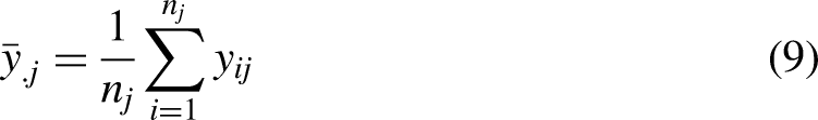$n_j$ individuals within intersection j yields the simple mean:

$${\overline{y}}_{.j}={\displaystyle \frac{1}{n_j}\sum _{i=1}^{n_j}{y}_{ij}}$$

(9)

This is sometimes referred to as the cross-classification method. The simple mean can also be obtained by estimating a linear regression of $y_{ij}$ on an intercept and $J-1$ dummy variables (or no intercept and J dummy variables) and predicting the fitted values, sometimes referred to as a fixed effects dummy variable model. Alternatively, they can be derived by fitting a linear regression of $y_{ij}$ on the social identity variables that define the intersections, fully interacting these variables. This is sometimes referred to as a saturated fixed effects model, and was until MAIHDA the cutting edge for quantitative intersectional analyses. For example, in the Keller et al. (2023) study, this would involve entering the main effects of the four social identity variables, and then all two-, three-, and four-way interactions terms.

MAIHDA Model 1 Means

The MAIHDA Model 1 mean for intersection j is defined as the conditional expectation of the true intersection mean, given the observed simple mean for that intersection:

$${\tilde{\mu }}_{1j}\equiv \mathrm{E}({\mu }_j|{\overline{y}}_{.j})=R_{1j}{\overline{y}}_{.j}+(1-R_{1j}){\beta }_{1,0}$$

(10)

where we use the tilde notation to help distinguish the predicted mean ${\tilde{\mu }}_{1j}$ from the true mean ${\mu }_j$ . Under frequentist estimation, we plug in the parameter estimates, resulting in empirical Bayes predictions. Under Bayesian estimation, we instead estimate the posterior distribution of ${\mu }_j$ and summarize it using the posterior mean.

The term $R_{1j}$ is the reliability of the simple mean ${\overline{y}}_{.j}$ as an estimate of the true mean ${\mu }_j$ . These predictions are therefore reliability-weighted averages of the simple means ${\overline{y}}_{.j}$ and the model-implied or overall mean ${\beta }_{1,0}$ . The more reliable ${\overline{y}}_{.j}$ is as an estimate of ${\mu }_j$ , the more weight is given to ${\overline{y}}_{.j}$ and the less to ${\beta }_{1,0}$ . The Model 1 means can therefore be viewed as a prediction that starts with the simple mean and is then shrunk toward the overall mean. The degree of shrinkage is given by:

$${\tilde{\mu }}_{1j}-{\overline{y}}_{.j}=(R_{1j}-1)({\overline{y}}_{.j}-{\beta }_{1,0})$$

(11)

Therefore, shrinkage decreases as reliability increases, and it also decreases as the difference between the simple mean and the overall mean becomes smaller.

Reliability is calculated as the ratio of the true mean variance to the observed mean variance, and thus varies from 0 to 1: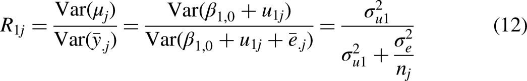

$$R_{1j}={\displaystyle \frac{\mathrm{Var}({\mu }_j)}{\mathrm{Var}({\overline{y}}_{.j})}={\displaystyle \frac{\mathrm{Var}({\beta }_{1,0}+u_{1j})}{\mathrm{Var}({\beta }_{1,0}+u_{1j}+{\overline{e}}_{.j})}={\displaystyle \frac{{\sigma }_{u1}^2}{{\sigma }_{u1}^2+{\displaystyle \frac{{\sigma }_e^2}{n_j}}}}}}$$

(12)

where ${\overline{e}}_{.j}$ is the mean of the individual residuals:

$${\overline{e}}_{.j}={\displaystyle \frac{1}{n_j}\sum _{i=1}^{n_j}{e}_{ij}}$$

(13)

with variance ${\sigma }_e^2/n_j$ . Note that we do not add a 1 subscript to ${\overline{e}}_{.j}$ or ${\sigma }_e^2$ , as these terms do not change when moving from Model 1 to Model 2. Reliability can also be interpreted as the squared correlation between ${\overline{y}}_{.j}$ and ${\mu }_j$ , that is, as the R-squared or coefficient of determination for predicting ${\mu }_j$ from ${\overline{y}}_{.j}$ . From this expression, we see that reliability increases with the Model 1 $\mathrm{VPC}$ , the magnitude of intersectional inequalities, and $n_j$ , the number of individuals at an intersection. This suggests that as VPC or $n_j$ increase, both ${\overline{y}}_{.j}$ and ${\tilde{\mu }}_j$ will converge toward ${\mu }_j$ .

MAIHDA Model 2 Means

The MAIHDA Model 2 mean for intersection j is given by the conditional expectation of the true mean, given the simple mean and the covariates for that intersection: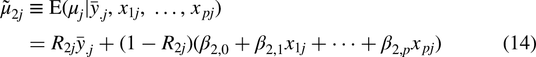

$${\tilde{\mu }}_{2j}\equiv \mathrm{E}({\mu }_j|{\overline{y}}_{.j},x_{1j},\dots ,x_{pj})=R_{2j}{\overline{y}}_{.j}+(1-R_{2j})({\beta }_{2,0}+{\beta }_{2,1}{x}_{1j}+\cdots +{\beta }_{2,p}{x}_{pj})$$

(14)

where $R_{2j}$ is the reliability of the simple mean ${\overline{y}}_{.j}$ as an estimate of the true mean ${\mu }_j$ , conditional on the additive effects of the multiple social identities. Thus, the Model 2 means are also weighted averages of the simple means ${\overline{y}}_{.j}$ and the model-implied means, but where the latter are now given by the fixed-part of the model ${\beta }_{2,0}+{\beta }_{2,1}{x}_{1j}+\cdots +{\beta }_{2,p}{x}_{pj}$ . Because the additive model implies a different mean for every intersection, the shrinkage is now towards a different point for every intersection rather than the single common point ${\beta }_{1,0}$ . The degree of shrinkage is now given by:

$${\tilde{\mu }}_{2j}-{\overline{y}}_{.j}=(R_{2j}-1)\{{\overline{y}}_{.j}-({\beta }_{2,0}+{\beta }_{2,1}{x}_{1j}+\cdots +{\beta }_{2,p}{x}_{pj})\}$$

(15)

and, therefore, again decreases as the now conditional reliability increases, and again increases as the difference between the simple mean and the model-implied mean increases.

The expression for the conditional reliability takes the same form as before: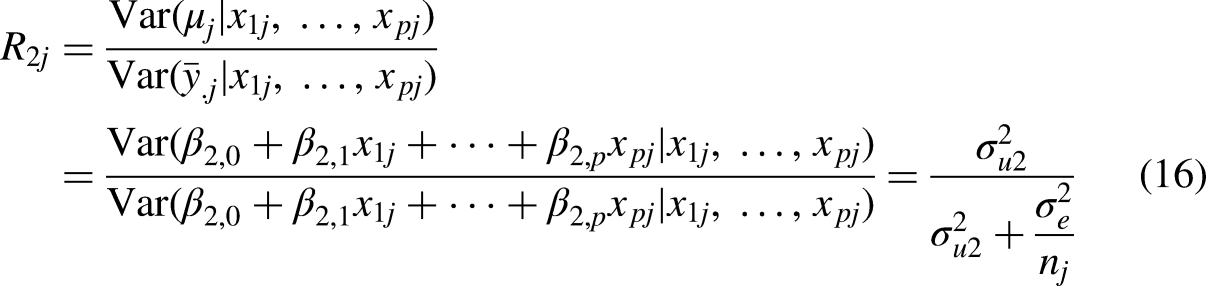

$$R_{2j}={\displaystyle \frac{\mathrm{Var}({\mu }_j|x_{1j},\dots ,x_{pj})}{\mathrm{Var}({\overline{y}}_{.j}|x_{1j},\dots ,x_{pj})}={\displaystyle \frac{\mathrm{Var}({\beta }_{2,0}+{\beta }_{2,1}{x}_{1j}+\cdots +{\beta }_{2,p}{x}_{pj}|x_{1j},\dots ,x_{pj})}{\mathrm{Var}({\beta }_{2,0}+{\beta }_{2,1}{x}_{1j}+\cdots +{\beta }_{2,p}{x}_{pj}|x_{1j},\dots ,x_{pj})}={\displaystyle \frac{{\sigma }_{u2}^2}{{\sigma }_{u2}^2+{\displaystyle \frac{{\sigma }_e^2}{n_j}}}}}}$$

(16)

However, the conditional reliabilities will have lower values than the unconditional reliabilities as ${\sigma }_{u2}^2<{\sigma }_{u1}^2$ . Specifically, as the explanatory power of the additive effects of the social identity variables increases, ${\sigma }_{u2}^2$ decreases, resulting in lower values of $R_{2j}$ . Consequently, when computing the MAIHDA means, the shrinkage factor in Model 2 is stronger than in Model 1, $|R_{2j}-1|>|R_{1j}-1|$ . However, because Model 2 typically shrinks the simple means toward more realistic values than Model 1—since the model-implied means in Model 2, based on additive effects, are generally more accurate for most intersections than the overall mean used in Model 1—the Model 2 shrinkage factors are typically applied to smaller differences between the simple means and model-implied means than in Model 1. Whether the resulting degree of shrinkage is generally larger or smaller in Model 1 or Model 2 depends on the specific application. In the presence of a very strong two-way interaction, the model-implied means from a more complex model that includes this interaction at a fixed-effect covariate will be even more realistic. However, even when Model 2 is misspecified by omitting this interaction, its model-implied means will generally provide more realistic values to shrink toward than simply shrinking to the overall intercept from Model 1.

Illustrative Application

Figure 2 focuses on the simple mean and the MAIHDA means from Models 1 and 2 for Intersection 37 (male, native, low parental education, high occupational status; n = 14) [Keller et al. (2023)]. The plot illustrates how the MAIHDA means for Models 1 and 2 (triangles) are reliability-weighted averages of the simple mean (circles) and their respective model-implied means (squares). For Model 1, the model-implied mean is the overall mean, whereas for Model 2, it is the mean implied by the estimated additive effects of being male, native, low parental education and high occupational status.

Figure 2.

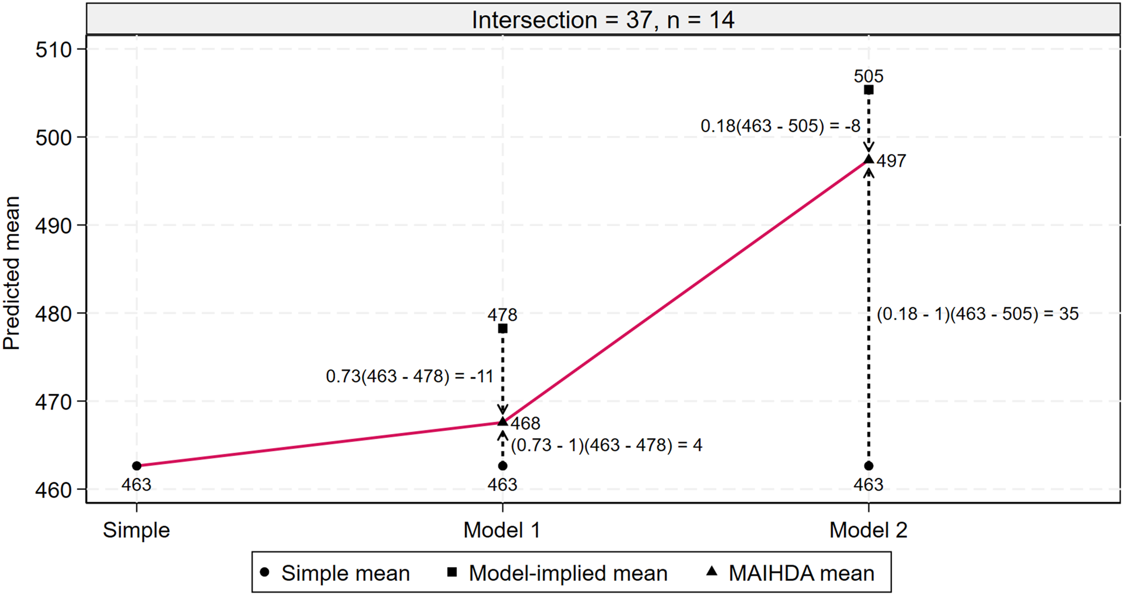
Predicted simple mean, multilevel analysis of individual heterogeneity and discriminatory accuracy (MAIHDA) model 1 mean, and MAIHDA model 2 mean for intersection 37 in the Keller et al. (2023) study. The plot illustrates how the MAIHDA Model 1 and Model 2 means are weighted averages of the simple mean and the corresponding model-implied mean. Intersection 37 includes male, native students with low parental education and high occupational status (n = 14).

In Model 1, the reliability of the simple mean is low (0.73) as it is based on only 14 individuals, and the simple mean of 463 is some 15 points lower than the model-implied mean of 478. As a result, the simple mean is shrunk upwards by 4 points towards the model-implied mean, resulting in a Model 1 MAIHDA mean of 468.

In Model 2, the conditional reliability of the simple mean is very low (0.18), and the simple mean of 463 is some 42 points lower than the model-implied mean of 505. As a result, the prediction is shrunk upwards by a very large 35 points towards the model-implied mean, resulting in a Model 2 MAIHDA mean of 497.

Reconsider the different predicted means for the six intersections plotted in Figure 1 and listed in Table 2. In Model 1, the MAIHDA means represent the simple means shrunk toward the overall model-implied mean of 478. The reliabilities and therefore the degree of multiplicative shrinkage vary as a function of intersection size from 0.36 to 0.73. In Model 2, the MAIHDA means are instead shrunk toward intersection-specific model-implied means derived from the additive model specification. The conditional reliabilities vary from 0.05 to 0.18. As expected, in both models, the MAIHDA means fall between the simple means and the model-implied means.

Analytic Expressions

Thus far, we have defined the Simple Means as well as the MAIHDA Model 1 and Model 2 means, shown that they yield different results, and demonstrated that these differences can be substantial—particularly for small intersectional groups—in a real-world setting. The remainder of the paper aims to evaluate and clarify the statistical properties of these three approaches to predicting intersectional group means. In doing so, we address our motivating questions: How much more accurate are MAIHDA means compared to simple means? What factors influence their relative accuracy? And, most importantly, is the choice between simple and MAIHDA means likely to affect conclusions in real-world research?

We use analytic expressions rather than simulations because they allow us to precisely identify the sources of divergence between the approaches and to assess their performance efficiently across a wide range of scenarios, in a way that prior simulation-based studies have struggled to do so. As with simulation studies, however, analytic approaches require specification of a “true” model or data-generating process (DGP) to serve as a benchmark. It is therefore important that the assumed DGP be a plausible reflection of reality.

MAIHDA Model 1 would be a poor choice, as it assumes no consistent (additive) patterns in intersectional inequalities. The simple means model is even less plausible, as it treats each intersectional group as entirely independent—an “island”—offering no information about any other group. In contrast, MAIHDA Model 2 provides a far more realistic basis, combining additive structure in intersectional inequalities with intersection-specific deviations. Empirical studies often find that 60–95% of the variation in intersectional inequalities is accounted for by additive effects, supporting the assumptions embedded in Model 2. Moreover, via shrinkage, MAIHDA Model 2 leverages information across groups, reflecting the idea that every intersectional group shares information with others. We therefore assume that the true DGP follows MAIHDA Model 2.

Of course, the true DGP is unknown in any applied study and will vary from case to case. It will also inevitably differ from MAIHDA Model 2 in some respects. The key point is that Model 2 will more closely resemble most real-world DGPs than either Model 1 or the Simple Means model.

Statistical Properties of the Distribution of Predicted Intersection Means

We begin our comparison of the statistical properties of three approaches to predicting intersection means by focusing on the big picture—how the approaches vary in capturing the distribution of intersection means.

We start by presenting analytical expressions for the variance of the intersection means across the distribution of intersections. We then graphically demonstrate how these variances change with intersection size and how these relationships are influenced by the Model 1 VPC, the Model 2 PCV, and the variability of intersection sizes. We operationalize the latter in terms of the coefficient of variation (CV) of intersection sizes, defined as the ratio of the SD of intersection sizes to the mean. A CV of 0 means all intersections are of equal size. But most applications have unequal intersection sizes and so CVs greater than 0. Finally, we provide analytical expressions for the correlation between each set of means and the true means, and illustrate these correlations graphically in a parallel manner. We do not present analytical expressions for the expectation of each set of means as in all cases the expectation is equal to the mean of the intersection means.

The analytic expressions we present follow from results in the statistical literature on multilevel models. To derive all expressions, we specify the true model as Model 2 and assume that the regression coefficients, intersection random effect variance, and individual residual variance are known, with only the true mean for each intersection being unknown. Thus, all derivations are done in terms of the true parameter values of Model 2, rather than in terms of frequentist or Bayesian estimators. Additionally, we assume many intersections of equal size. We present full derivations in the online supplements. We use simulation to address the case of varying intersection sizes. For plotting purposes, we consider the case where the mean and SD of the outcome are 0 and 1, respectively.

Variance of the Predicted Means Across the Distribution of Intersections

Let 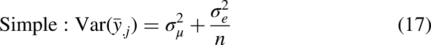${\sigma }_{\mu }^2$ denote the variance of the true means. The variance of each set of predicted means can then be written as:

$$\mathrm{Simple}:\mathrm{Var}({\overline{y}}_{.j})={\sigma }_{\mu }^2+{\displaystyle \frac{{\sigma }_e^2}{n}}$$

(17)

$$\mathrm{Model}1:\mathrm{Var}({\tilde{\mu }}_{1j})=R_1{\sigma }_{\mu }^2$$

(18)

$$\mathrm{Model}2:\mathrm{Var}({\tilde{\mu }}_{2j})={\sigma }_{\mu }^2-(1-R_2){\sigma }_{u2}^2$$

(19)

where we continue to use $1$ and $2$ subscripts to distinguish between the Model 1 and Model 2 parameters, with the exception for ${\sigma }_e^2$ , as ${\sigma }_{e1}^2={\sigma }_{e2}^2$ . Since we assume balanced data, we omit the j subscript from n, $R_1$ and $R_2$ .

Figure 3 shows the true variance and the variances of the Simple, Model 1, and Model 2 predicted means, plotted against intersection size. The figure is based on a Model 1 VPC of 0.15, a Model 2 PCV of 0.90, and a CV of intersection sizes of 0, indicating equal intersection sizes. These VPC and PCV values are similar to those reported in Keller et al. (VPC = 0.16 and PCV = 0.91). The CV value differs from that reported in Keller et al., where the CV was 0.98. We plot the four variances against intersection size only up to $n=100$ because the differences between the variances diminish as intersection size increases. In Keller et al., the sizes of the 40 intersections ranged from 3 to 512 students, with a median of 93. Six intersections had fewer than 20 students, and three had fewer than 10.

Figure 3.

Variance of the simple means (17), MAIHDA model 1 means (18), and MAIHDA model 2 means (19) across the distribution of intersections, plotted against intersection size. The plot assumes a Model 1 VPC of 0.15, a Model 2 PCV of 0.90, and equal intersection sizes. MAIHDA: multilevel analysis of individual heterogeneity and discriminatory accuracy; PCV: proportion change in variance; VPC: variance partition coefficient.

Given the Model 1 VPC of 0.15 and an outcome variance of 1, it follows that the variance of the true means is also 0.15. This variance remains constant regardless of intersection size. In contrast, the variance of the simple means is initially much larger but decreases as intersection size increases, eventually converging to the true variance. This follows from the expression: $\mathrm{Var}({\overline{y}}_{.j})={\sigma }_{\mu }^2+{\sigma }_e^2/n$ . As $n\to \mathrm{\infty }$ , the term ${\sigma }_e^2/n\to 0$ , leading to $\mathrm{Var}({\overline{y}}_{.j})\to {\sigma }_{\mu }^2$ . In words, the variance of the simple means is equal to the sum of the true variance and the sampling variance in the simple mean. The latter tends to 0 as the number of individuals per intersection increases. Thus, with sufficiently large intersection sizes, the variance of the simple means approaches that of the true means. However, when intersection sizes are smaller, the variance of the simple means overestimates the true variance.

The variance of the Model 1 means is smaller than the true variance when n is small, but it increases and converges to the true variance as intersection size increases. This follows from the expression: $\mathrm{Var}({\tilde{\mu }}_{1j})=R_1{\sigma }_{\mu }^2$ . As $n\to \mathrm{\infty }$ , the term $R_1\to 1$ , leading to $\mathrm{Var}({\tilde{\mu }}_{1j})\to {\sigma }_{\mu }^2$ . Thus, with sufficiently large intersection sizes, the reliabilities approach 1, and so the variance of the Model 1 means also closely approximates the variance of the true means. The fact that the variance of the Model 1 means is smaller than the true variance reflects the conservative nature of shrinkage—shrinkage leads to an underestimation of the true variance, particularly when intersection size is small. Importantly, for any given intersection size, while the variance of the Model 1 means is biased downward, it remains closer to the true variance than the variance of the simple means, which is biased upward.

The variance of the Model 2 means is slightly smaller than the true variance when n is small, but it increases and converges to the true variance as intersection size increases. Compared to Model 1, the variance of the Model 2 means remains close to the true variance even at the smallest intersection sizes. This is because the PCV is 0.90, indicating that 90% of the variation in the Model 2 means is captured by additive social identity effects, which are identified using data pooled across all intersections, and therefore reliably. Only 10% of the variation stems from intersection-specific deviations, which are identified separately for each intersection. As a result, relatively little data per intersection is required for the variance of the Model 2 means to approximate the true variance.

In summary, the variance of the simple means is biased upwards, whereas the variances of the Model 1 and Model 2 means are biased downwards. The magnitude of all three biases decreases as intersection size increases. However, the variance of the Model 2 means is always closest to the variance of the true means (i.e., shows the smallest bias). Thus, regardless of intersection size, the Model 2 means are the preferred means to report. These results have implications for the reporting of tables of intersection means.

Figure 3 was plotted using specific values for the Model 1 VPC, Model 2 PCV, and CV of intersection size. Supplemental Figures S1, S2, and S3 in the online supplements explore how this plot changes as each of these factors varies. The key finding is that the relative ranking of the three methods of prediction remains unchanged. However, the advantage of the Model 2 mean over the simple mean is most pronounced when intersectional inequalities are less pronounced (low VPC), when inequalities follow a largely additive pattern (high PCV), and when intersections vary in size (high CV).

Correlation Between the Predicted and True Means Across the Distribution of Intersections

The correlation of each set of predicted means with the true means is given by:

$$\mathrm{Simple}:\mathrm{Corr}({\overline{y}}_{.j},{\mu }_j)=\sqrt{R_1}$$

(20)

$$\mathrm{Model}1:\mathrm{Corr}({\tilde{\mu }}_{1j},{\mu }_j)=\sqrt{R_1}$$

(21)

$$\mathrm{Model}2:\mathrm{Corr}({\tilde{\mu }}_{2j},{\mu }_j)=\sqrt{\mathrm{PCV}+R_2(1-\mathrm{PCV})}$$

(22)

The higher the correlation, the more the set of predicted means reflect the distribution of true means.

Figure 4 shows the correlation between each set of predicted means and the true means, plotted against intersection size. The figure is based on a Model 1 VPC of 0.15, a Model 2 PCV of 0.90, and a CV of intersection size of 0, indicating equal intersection sizes.

Figure 4.

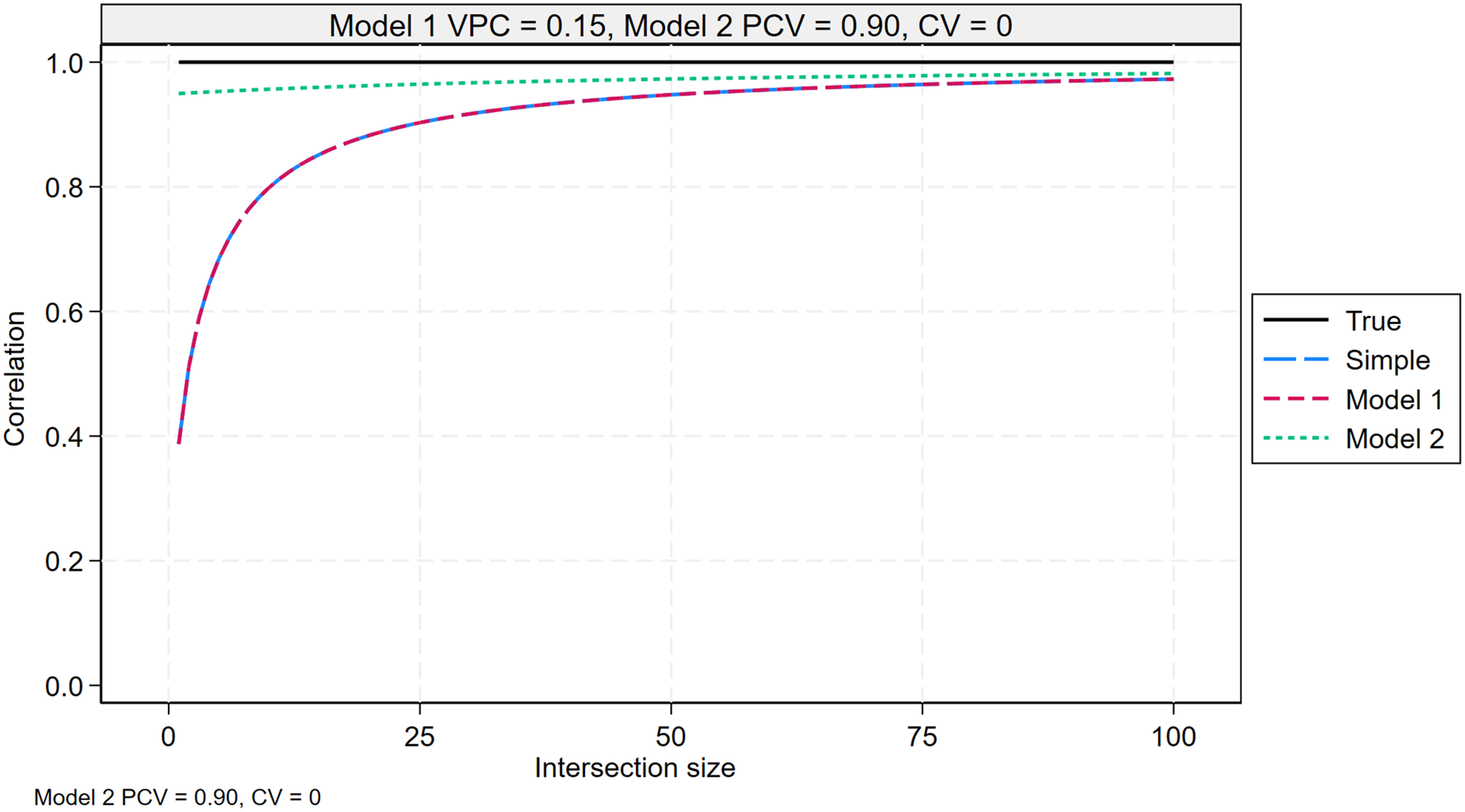
Correlation between the simple means and the true means (20), MAIHDA model 1 means and the true means (21), and MAIHDA model 2 means and the true means (22), across the distribution of intersections, plotted against intersection size. The plot assumes a Model 1 VPC of 0.15, a Model 2 PCV of 0.90, and equal intersection sizes. The line plots for the simple means and the MAHDA Model 1 means lie on top of one another. MAIHDA: multilevel analysis of individual heterogeneity and discriminatory accuracy; PCV: proportion change in variance; VPC: variance partition coefficient.

The correlation between the simple means and the true means is initially much smaller than 1 but increases as intersection size grows, eventually converging to a correlation of 1. The low correlation at smaller intersection sizes reflects the low reliability of the simple means as a predictor of the true means when intersection sizes are small. As $n\to \mathrm{\infty }$ , $R_1\to 1$ , leading to $\mathrm{Corr}({\overline{y}}_{.j},{\mu }_j)\to 1$ . Thus, with sufficiently large intersection sizes, the correlation between the simple means and the true means approaches 1.

Figure 4 shows the correlation between the Model 1 means and the true means is identical to the correlation between the simple means and the true means (their respective line plots lie on top of one another). This is because, in the current case of equal intersection sizes, the Model 1 means are just the simple means shrunk towards the overall mean by a common reliability statistic. The two correlations will diverge when we allow the intersection sizes to vary (as seen in Supplemental Figure S6 and discussed below).

The correlation between the Model 2 means and the true means also converges to a correlation of 1 as intersection sizes increase. Compared to Model 1, the correlation between the Model 2 means and the true means remains close to 1 even at the smallest intersection sizes. This is due to the PCV being 0.90, which means that 90% of the variation in the Model 2 means is explained by additive social identity effects, identified using data pooled across all intersections, and therefore reliably. Only 10% of the variation stems from intersection-specific deviations, which are identified separately for each intersection. As a result, relatively little data per intersection is needed for the correlation between the Model 2 means and the true means to be close to 1.

In summary, all three correlations are biased downwards but approach 1 as intersection size increases. The correlation between the Model 2 means and the true means consistently shows the smallest bias. Therefore, the Model 2 means are the preferred predictor to report, regardless of intersection size.

Figure 4 was plotted using specific values for the Model 1 VPC, Model 2 PCV, and CV of intersection size. Supplemental Figures S4, S5, and S6 in the online supplements explore how this plot changes as each of these factors varies. The key finding is that the Model 2 means remain the preferred predictor. However, similar to the variance of the predicted means, the advantage of this predictor is most pronounced when intersectional inequalities are less pronounced (low VPC), when inequalities follow a largely additive pattern (high PCV), and when intersections vary in size (high CV).

Statistical Properties of Predicted Intersection Mean for a Given Intersection

In this section, we continue to address the same two key questions: Which set of predicted means—Simple, Model 1, or Model 2—is most appropriate to report, and does this choice depend on the nature of intersectional inequalities—magnitude and additivity—being studied and the size of the data? However, our goal here is to examine the statistical properties of the predicted mean for a given intersection across random samples of individuals from that intersection. This contrast, the previous section where we focused on the statistical properties of the distribution of predicted intersection means across the population of intersections.

We focus on the bias, variance, and MSE of each predictor for a given intersection. Bias measures the difference between the average predicted mean for a given intersection and its true value. A high bias, whether positive or negative, means the predictor consistently over- or under-predicts. Variance here reflects how much the predicted intersection mean varies across different samples of individuals. In other words, if we were to repeat a sampling process multiple times from the same intersection population, how varied would our predictions be? High variance indicates that the model is overly sensitive to the specific individuals randomly selected for the sample. Importantly, when comparing predictors there is typically a bias-variance tradeoff whereby the only way to reduce the variance is by introducing bias. The MSE therefore combines both bias and variance to assess overall prediction accuracy, with a lower MSE indicating better predictive performance.

We begin by presenting analytic expressions for the bias, variance, and MSE. As in the previous section, the analytic expressions we present follow from results in the statistical literature on multilevel models. We again present full derivations in the online supplements. After presenting analytic expressions for bias, variance, and MSE, we graphically illustrate how these properties change as a function of the difference between the true intersection mean and the model-implied mean and how these relationships are influenced by intersection size, the Model 1 VPC, and the Model 2 PCV.

To derive all expressions, we continue to specify the true model as Model 2 and assume that the regression coefficients, intersection random effect variance, and individual residual variance are known, with only the true mean for each intersection being unknown. For plotting purposes, we again consider the case where the mean and SD of the outcome are 0 and 1, respectively.

Bias

For each predictor, the bias for intersection j measures the difference between the expected value for the predicted mean and the true mean for that intersection:

$$\mathrm{Simple}:\mathrm{bias}({\overline{y}}_{.j}|{\mu }_j)=0$$

(23)

$$\mathrm{Model}1:\mathrm{bias}({\tilde{\mu }}_{1j}|{\mu }_j)=-(1-R_{1j})({\mu }_j-{\beta }_{1,0})$$

(24)

$$\mathrm{Model}2:\mathrm{bias}({\tilde{\mu }}_{2j}|{\mu }_j)=-(1-R_{2j})\{{\mu }_j-({\beta }_{2,0}+{\beta }_{2,1}{x}_{1j}+\cdots +{\beta }_{2,p}{x}_{pj})\}$$

(25)

where the $1$ and $2$ subscripts continue to distinguish between the Model 1 and Model 2 parameters.

Figure 5 presents the bias of each predictor as a function of the difference between the true mean ${\mu }_j$ and the model-implied mean for that intersection: ${\beta }_{1,0}$ in Model 1 or ${\beta }_{2,0}+{\beta }_{2,1}{x}_{1j}+\cdots +{\beta }_{2,p}{x}_{pj}$ in Model 2. The figure assumes an intersection size of 10 individuals, a Model 1 VPC of 0.15, and a Model 2 PCV of 0.90. It follows that the Model 1 and 2 reliabilities are 0.64 and 0.15. Notably, in the Keller et al. study, six of the 40 intersections had fewer than 20 students, and three had fewer than 10 students. The x-axis range of the plots for the Simple and Model 1 bias are limited to the expected middle 95% of differences from Model 1, given by $\pm {\mathrm{\Phi }}^{-1}(0.975)\sqrt{{\sigma }_{u1}^2}$ . Similarly, the x-axis range for the plot of the Model 2 bias is restricted to the expected middle 95% of differences from Model 2, given by $\pm {\mathrm{\Phi }}^{-1}(0.975)\sqrt{{\sigma }_{u2}^2}$ . We apply these limits to avoid disproportionately long bias lines (and variance and MSE lines in Figures 6 and 7) at the extremes, which could distract the reader from the main patterns within the central range of the data.

Figure 5.

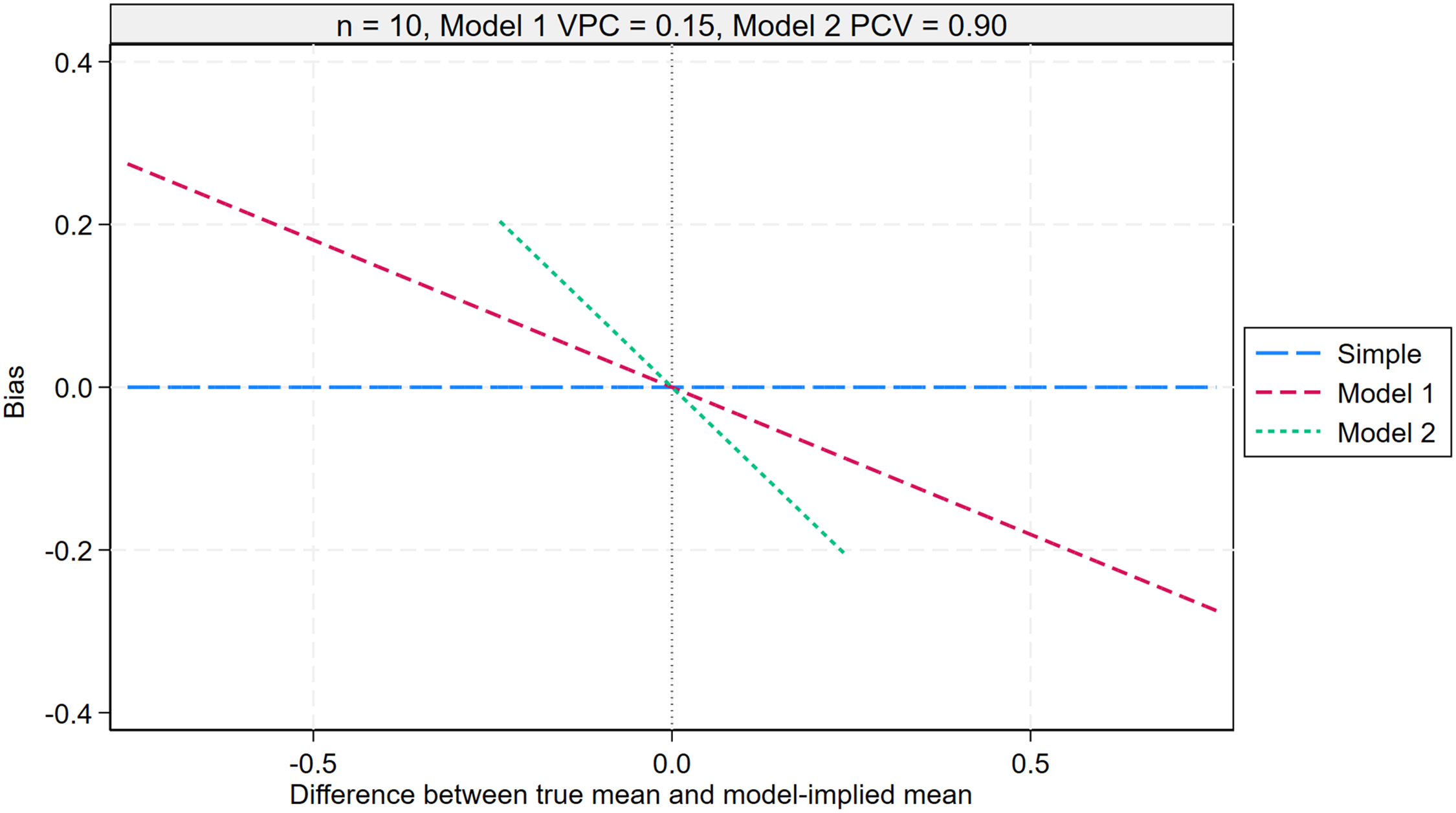
Bias of the simple mean (23), MAIHDA model 1 mean (24), and MAIHDA model 2 mean (25) across repeated samples of individuals for a given intersection, plotted against the difference between the true mean and the model-implied mean for that intersection. The plot assumes an intersection size of 10 individuals, a Model 1 VPC of 0.15, and a Model 2 PCV of 0.90. The Model 1 model-implied mean corresponds to the overall mean, while the Model 2 model-implied mean reflects the additive effects of the social identities defining the intersection. The bias of the MAIHDA Model 2 mean is shown over a narrower range due to smaller differences between the true and model-implied means in this model. MAIHDA: multilevel analysis of individual heterogeneity and discriminatory accuracy; PCV: proportion change in variance; VPC: variance partition coefficient.

Figure 6.

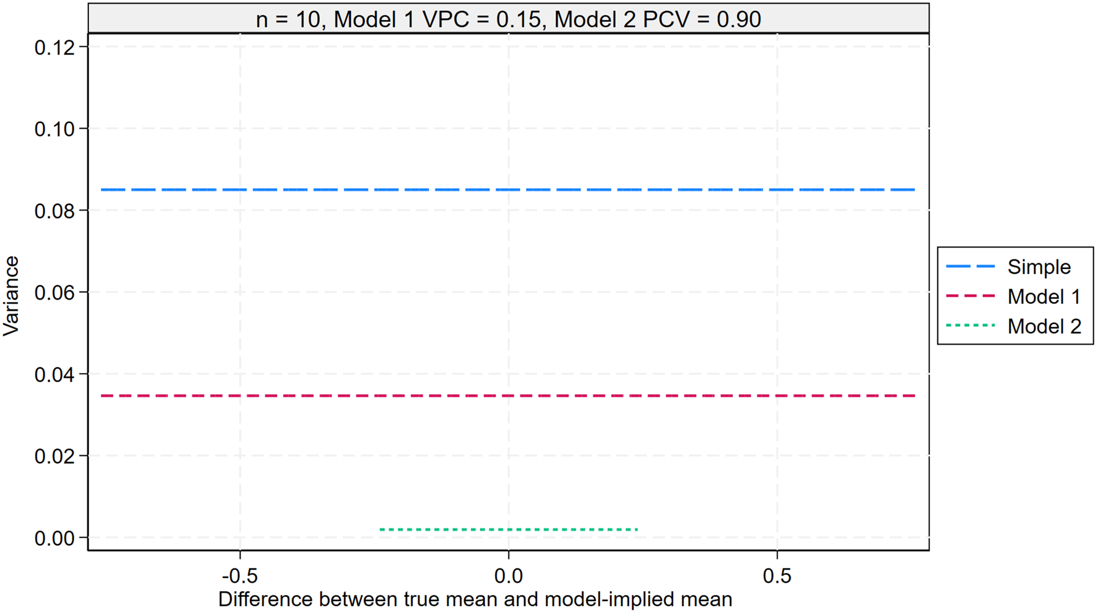
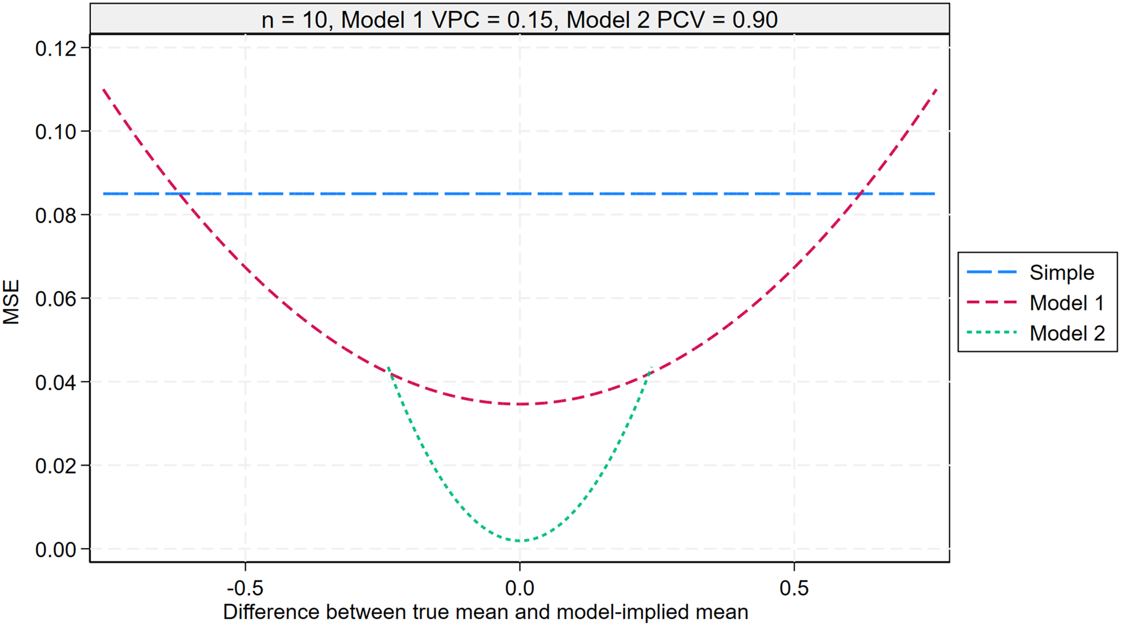
Variance of the simple mean (26), MAIHDA model 1 mean (27), and MAIHDA model 2 mean (28) across repeated samples of individuals for a given intersection, plotted against the difference between the true mean and the model-implied mean for that intersection. The plot assumes an intersection size of 10 individuals, a Model 1 VPC of 0.15, and a Model 2 PCV of 0.90. The Model 1 model-implied mean corresponds to the overall mean, while the Model 2 model-implied mean reflects the additive effects of the social identities defining the intersection. The bias of the MAIHDA Model 2 mean is shown over a narrower range due to smaller differences between the true and model-implied means in this model. MAIHDA: multilevel analysis of individual heterogeneity and discriminatory accuracy; PCV: proportion change in variance; VPC: variance partition coefficient.

Figure 7.

Mean squared error of the simple mean (29), MAIHDA model 1 mean (30), and MAIHDA model 2 mean (31) across repeated samples of individuals for a given intersection, plotted against the difference between the true mean and the model-implied mean for that intersection. The plot assumes an intersection size of 10 individuals, a Model 1 VPC of 0.15, and a Model 2 PCV of 0.90. The Model 1 model-implied mean corresponds to the overall mean, while the Model 2 model-implied mean reflects the additive effects of the social identities defining the intersection. The bias of the MAIHDA Model 2 mean is shown over a narrower range due to smaller differences between the true and model-implied means in this model. MAIHDA: multilevel analysis of individual heterogeneity and discriminatory accuracy; PCV: proportion change in variance; VPC: variance partition coefficient.

The simple mean is an unbiased predictor of the true mean, meaning that, averaging across repeated samples, the simple mean equals the true mean.

The Model 1 mean is a biased predictor. The bias is a negative linear function of the difference between the true mean ${\mu }_j$ and the model-implied mean ${\beta }_{1,0}$ , where the latter is simply the overall mean. Specifically, this difference is scaled by $-(1-R_{1j})$ , which is negative and, in this illustration takes the value −0.36 (with a possible range from −1 to 0). As a result, the sign of the difference is reversed, and its magnitude is reduced. Consequently, when the true mean exceeds the model-implied mean, the Model 1 mean is biased downward, whereas when the true mean is lower than the model-implied mean, the bias is upward. Thus, the Model 1 is biased toward the model-implied mean. This once again reflects the conservative nature of shrinkage.

The Model 2 mean is also a biased predictor of the true mean, with the magnitude of its bias again following a negative linear relationship with the difference between the true mean ${\mu }_j$ and the model-implied mean ${\beta }_{2,0}+{\beta }_{2,1}{x}_{1j}+\cdots +{\beta }_{2,p}{x}_{pj}$ . However, unlike in Model 1, the model-implied mean is now an intersection-specific mean, determined by the additive effects of the relevant social identity characteristics. As a result, these model-implied means are typically closer to the true means than in Model 1. This increases the first term in absolute magnitude and decreases the second term in the expression for the bias. Specifically, the first term, $-(1-R_{2j})$ , is now −0.85. It is now closer to −1 because the conditional reliability $R_{2j}$ is always lower than the unconditional reliability $R_{1j}$ . This results in a larger per-unit multiplicative bias, making the slope of the linear bias relationship steeper than before. However, the decrease in the second term—the deviation between the true and model-implied mean—means this increased multiplier is applied to smaller differences than in Model 1, making the range over which the linear bias relationship operates narrower (note the narrower range of the line plot for Model 2 in Figure 5). The net effect is that the Model 2 mean is expected to be a less biased predictor of the true mean for a given intersection than the Model 1 mean. Nevertheless, the Model 2 mean remains a biased predictor, and one that is biased towards additivity. That is, the predicted intersection means will conform more to additivity than they do in actuality.

In summary, the simple mean is an unbiased predictor of the true intersection mean, whereas the Model 1 and Model 2 means are both biased towards their respective model-implied means with the Model 1 means, on average, exhibiting greater bias.

Supplemental Figures S7, S8, and S9 in the online supplements explore how the results shown in Figure 5 change as a function of intersection size, Model 1 VPC, and Model 2 PCV. The key finding is that the simple mean remains the preferred predictor as it is always unbiased (when averaged across repeated samples), whereas the Model 1 and Model 2 means exhibit bias in all cases except when the true and model-implied means are equal.

Variance

For each predictor, the variance for intersection j measures the variability of the prediction (their “consistency”) across random samples of individuals from that intersection: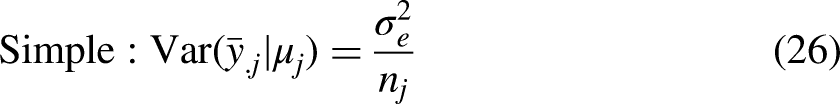

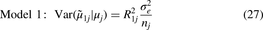
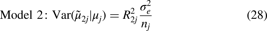
$$\mathrm{Simple}:\mathrm{Var}({\overline{y}}_{.j}|{\mu }_j)={\displaystyle \frac{{\sigma }_e^2}{n_j}}$$

(26)

$$\mathrm{Model}1:\mathrm{Var}({\tilde{\mu }}_{1j}|{\mu }_j)=R_{1j}^2{\displaystyle \frac{{\sigma }_e^2}{n_j}}$$

(27)

$$\mathrm{Model}2:\mathrm{Var}({\tilde{\mu }}_{2j}|{\mu }_j)=R_{2j}^2{\displaystyle \frac{{\sigma }_e^2}{n_j}}$$

(28)

Figure 6 presents the variance of each predictor for the true mean of intersection j as a function of the difference between the true mean and the model-implied mean for that intersection. The plot's range is again restricted to the expected middle 95% of differences for each model. As with the bias figure, the analysis assumes an intersection size of 10 individuals, a Model 1 VPC of 0.15, and a Model 2 PCV of 0.90.

The variance of each predictor is constant. For the simple mean, the variance is given by the sampling variance across repeated samples, $\frac{{\sigma }_e^2}{n_j}$ . The variance of the Model 1 mean is obtained by multiplying this sampling variance by the squared reliability, $R_{1j}^2$ which in this illustration is 0.38. As $R_{1j}<1$ , the Model 1 mean exhibits less variation across repeated samples than the simple mean —specifically, 62% less. The variance of the Model 2 mean follows the same general form as the Model 1 mean. However, because the conditional reliability is lower than the unconditional reliability, $R_{2j}<R_{1j}$ , the variance of the Model 2 mean is even smaller than that of Model 1. In this illustration, $R_{2j}^2=0.0225$ , meaning the variance of the Model 2 mean is 97.5% smaller than that of the simple mean.

In summary, the Model 2 mean has the lowest variance (the most consistency) across repeated samples, followed by the Model 1 mean, with the simple mean exhibiting the highest variance (least consistency). Thus, the Model 2 means to a much greater extent replicate themselves across repeated samples. The simple means do not.

Supplemental Figures S10, S11, and S12 explore how the results shown in Figure 6 change as a function of the intersection size, Model 1 VPC, and Model 2 PCV. The key finding is that the Model 2 mean remains the preferred predictor in terms of having the smallest variance. However, its advantage over the simple mean is most pronounced when the intersection size is small, intersectional inequalities are less pronounced (low VPC), and when these inequalities follow a largely additive structure (high PCV).

Mean Squared Error

For each predictor, the MSE for intersection j reflects both its variance and bias. As a result, the MSE provides a measure of the predictor's overall accuracy. A lower MSE indicates a more accurate predictor. Specifically, the MSE is defined as the sum of the variance and the bias squared: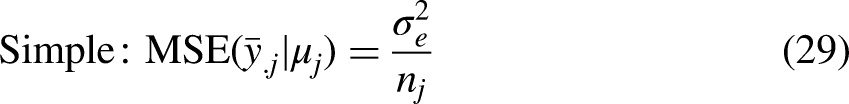

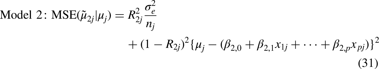
$$\mathrm{Simple}:\mathrm{MSE}({\overline{y}}_{.j}|{\mu }_j)={\displaystyle \frac{{\sigma }_e^2}{n_j}}$$

(29)

$$\mathrm{Model}1:\mathrm{MSE}({\tilde{\mu }}_{1j}|{\mu }_j)=R_{1j}^2{\displaystyle \frac{{\sigma }_e^2}{n_j}+(1-R_{1j}{)}^2({\mu }_j-{\beta }_{1,0}{)}^2}$$

(30)

$$\mathrm{Model}2:\mathrm{MSE}({\tilde{\mu }}_{2j}|{\mu }_j)=R_{2j}^2{\displaystyle \frac{{\sigma }_e^2}{n_j}+(1-R_{2j}{)}^2\{{\mu }_j-({\beta }_{2,0}+{\beta }_{2,1}{x}_{1j}+\cdots +{\beta }_{2,p}{x}_{pj}){\}}^2}$$

(31)

Figure 7 presents the MSE of each predictor for the true mean of intersection j as a function of the difference between the true mean and the model-implied mean for that intersection. The plot's range is again restricted to the expected middle 95% of differences for each model, and the analysis continues to assume an intersection size of 10 individuals, a Model 1 VPC of 0.15, and a Model 2 PCV of 0.90.

The MSE for the simple mean is equal to its variance, as its bias is zero.

The MSE for the Model 1 mean follows a quadratic function of the difference between the true mean and the model-implied mean, ${\mu }_j-{\beta }_{1,0}$ , where the model-implied mean is simply the overall mean. The MSE reaches its minimum when the true mean matches the model-implied mean, at which point it equals the variance of the Model 1 mean, $R_{1j}^2\frac{{\sigma }_e^2}{n_j}$ . As the true mean deviates from the model-implied mean, the MSE increases.

Similarly, the MSE for the Model 2 mean is also a quadratic function of the difference between the true mean and the model-implied mean. However, in this case, the model-implied mean represents the intersection-specific mean, determined by the additive effects of the relevant social identity characteristics, ${\beta }_{2,0}+{\beta }_{2,1}{x}_{1j}+\cdots +{\beta }_{2,p}{x}_{pj}$ . As with the Model 1 mean, the MSE is minimized when the true mean matches the model-implied mean, at which point it equals the variance of the Model 2 mean, $R_{2j}^2\frac{{\sigma }_e^2}{n_j}$ . Since this variance is lower than that of the Model 1 mean, the MSE for Model 2 at this point is also lower.

While the MSE of the Model 2 mean increases more rapidly than that of the Model 1 mean as the true mean increasingly deviates from the model-implied mean, this effect is mitigated by the fact that the model-implied means in Model 2 are generally much closer to the true means than those in Model 1. As a result, the MSE for the Model 2 mean will almost always be smaller than that for the Model 1 mean for a given intersection.

In summary, when the model-implied mean is closer to the true mean, both the Model 1 and, especially, Model 2 predictors exhibit lower MSE than the simple mean. As the model-implied mean deviates further from the true mean, the MSE for both models increases. However, the ranking of prediction method remains consistent, except in cases of extreme deviations. For instance, consider an intersection with a very low true mean of −0.7. Across repeated samples of 10 individuals, the MSE for the Model 1 mean at that intersection (0.099) would actually exceed that of the simple mean (0.085). However, the MSE for the Model 2 mean would be significantly lower.

Supplemental Figures S13, S14, and S15 explore how the results shown in Figure 7 change as a function of the intersection size, Model 1 VPC, and Model 2 PCV. The key finding is that the Model 2 mean remains the preferred predictor in terms of the lowest MSE. However, its advantage over the simple mean is most pronounced when intersection sizes are small, intersectional inequalities are less pronounced (low VPC), and the inequalities follow an additive structure (high PCV). These results align with the variance patterns observed earlier.

Discussion

This article examines the claim that the predicted intersection means derived from MAIHDA analysis provide better predictions of population intersection means than the simple arithmetic means. This claim is made in many applications of MAIHDA (Evans et al. 2024b) based on findings from the statistical literature on multilevel models, but until now this claim has not been formally explored in the context of MAIHDA analyses.

Our conclusion is that the predicted means from MAIHDA Model 2 are statistically more accurate than those from MAIHDA Model 1, and both outperform the simple means. This conclusion assumes that Model 2—which treats the additive main effects as fixed effects and all remaining two-way and higher-order interaction variability as an intersection-specific random effect—adequately represents the true DGP, a point we elaborate on below. Specifically, the Model 2 means exhibit the closest variance to, and the highest correlation with, the true means. While the Model 2 mean for a given intersection is biased (unlike the simple mean), it displays much lower variance across repeated samples, resulting in a lower MSE and, therefore, greater predictive accuracy. In essence, we accept a slight bias toward additivity in exchange for a substantial reduction in statistical noise. The improved statistical accuracy of the Model 2 means over the simple means arises from their ability to optimally combine the imprecise, intersection-specific simple means with precise, model-implied means that draw on information from all intersections.

This ranking of prediction methods holds across several key factors, including intersection size, the magnitude of these inequalities as measured by the VPC, the extent to which inequalities are driven by the additive effects of the social identities that form the intersections, as indicated by the PCV, and the variation in intersection sizes, measured by the CV.

Importantly, when all intersection sizes are large, the differences between the three methods diminish, making even the simple means reasonably accurate. However, when at least some intersection sizes are small, the difference in predicted intersection means become pronounced, particularly when the VPC is low and the PCV is high. Crucially, small intersection sizes, low VPCs, and high PCVs are very common in empirical MAIHDA applications (Evans et al. 2024a). Indeed, the intersections of the very greatest interest—those representing multiply marginalized groups—tend to be the very smallest, and so most sensitive to choice of prediction method.

Our analytical expressions are derived under the assumption that Model 2 is the DGP. In any real-world application, however, Model 2 can only approximate the unknown true DGP. Consequently, the greater the divergence of the real-world DGP from Model 2, the more likely it is that a more complex model could yield statistically more accurate estimates of intersectional means. For instance, in a particular application where a specific two-way interaction—such as that between gender and race—is substantial and supported by sufficient data, the true DGP might be better approximated by modeling this interaction as a fixed effect regression coefficient, rather than implicitly treating it as random, as in our current formulation.

However, the increase in predictive accuracy from specifying such a two-way interaction as fixed is likely to be relatively small compared to that achieved with the MAIHDA Model 2 means—and certainly smaller than the gains observed when moving from Simple Means to MAIHDA Model 1 means, and then to Model 2. The intuition is that, in most applications, the additive main effects in MAIHDA Model 2 account for approximately 60–95% of the variation in intersectional inequalities—a substantial to very large majority. This leaves limited room for further improvements in predictive accuracy by explicitly modeling specific interactions rather than absorbing them into the random effect. We illustrate this argument using a specific fixed two-way interaction DGP in the online supplements.

Nonetheless, it is important to further explore these and other arguments. In particular, it will likely be most informative to examine how the increase in predictive accuracy for a given intersection varies depending on how that intersection is involved in the specific two-way interaction. A key challenge in such explorations is that, as the true model becomes more complex, analytical derivations become increasingly difficult. In these cases, simulation studies will likely be necessary to assess the statistical properties of the resulting approaches.

As our analytic expressions relate to these true parameters, we have largely abstracted from the choice of estimation method. However, for the purpose of inference, this choice is important, as different estimation methods—frequentist approaches such as MLE and REML followed by empirical Bayes prediction, versus Bayesian methods such as MCMC—differ in how they propagate uncertainty in the estimated parameters into the predicted intersection effects. ML does not propagate uncertainty in the estimation of any model parameters. REML propagates uncertainty in the regression coefficients but not in the variance components. In contrast, Bayesian methods propagate uncertainty in all parameters. As a result, in any applied analysis, REML—and especially MLE—tend to understate uncertainty around the predicted intersection means. This would be expected to lead to Type I errors of inference—declaring particular intersections to show statistically significant deviations from additivity when they don’t. In this regard, Bayesian methods are preferable for MAIHDA analyses. Here too, simulation studies could be used to explore and quantify these differences and their implications.

While we focused on MAIHDA models for continuous outcomes, we see no reason why our findings will not apply more generally to MAIHDA models for binary (Evans et al. 2024b; Mahendran, Lizotte and Bauer 2022b) or other categorical, count, or survival outcomes. Similarly, we see no reason why they will not also apply to longitudinal MAIHDA models which fit separate mean trajectories for each intersection (Bell et al. 2024), or other random slope models. Future studies should confirm these intuitions. Our findings are also applicable when MAIHDA is used beyond intersectionality research, in the broader study of high-dimensional interactions among multiple categorical variables. Such applications have been termed multicategorical MAIHDA, to distinguish them from those focused specifically on intersectionality (Evans 2024; Rodriguez-Lopez et al. 2023).

Viewed more broadly, MAIHDA applies shrinkage to simple means through multilevel modeling. When recast as a linear regression of the outcome on a full set of intersection dummy variables, this process shrinks the estimated coefficients toward the overall mean, effectively functioning as a form of regularized regression. This perspective highlights the potential of alternative approaches—such as LASSO, Ridge regression, or elastic net—to achieve similar goals whether for continuous or other outcome types (Hastie, Tibshirani and Wainwright 2015). By fitting these models and using their predicted values, one will typically again obtain improved estimates of intersection means over the simple means. Future work might therefore also explore how these regularization methods compare to MAIHDA in terms of predictive accuracy and interpretability.

We have highlighted the benefits of shrinkage for predicting intersection means. However, shrinkage introduces a potential theoretical tension. Intersectionality emphasizes that unique combinations of social identities give rise to distinct lived experiences and, consequently, different outcomes. Yet, shrinkage pulls estimates for specific intersections toward the overall pattern across all intersections, which may seem to undermine the uniqueness of those experiences. This is the bias–variance tradeoff. To achieve greater predictive accuracy, we must accept some bias in exchange for substantially reduced variance. In our analysis, we have used minimization of the MSE as the criterion for balancing bias and variance. However, we acknowledge that some intersectionality researchers may wish to prioritize unbiasedness over predictive accuracy. In such cases, simple means may be preferable.

In sum, for optimal prediction of intersection means, we recommend using MAIHDA Model 2 over both Model 1 and simple means, especially when inequalities are subtle—whether in magnitude or due to hidden processes affecting specific combinations of social identities—and when data for certain intersections, such as those representing multiply marginalized groups, is limited.

Supplemental Material

sj-pdf-1-smr-10.1177_00491241251385123 - Supplemental material for The Statistical Advantages of Multilevel Analysis of Individual Heterogeneity and Discriminatory Accuracy for Estimating Intersectional Inequalities

Supplemental material, sj-pdf-1-smr-10.1177_00491241251385123 for The Statistical Advantages of Multilevel Analysis of Individual Heterogeneity and Discriminatory Accuracy for Estimating Intersectional Inequalities by George Leckie, Andrew Bell, Juan Merlo, SV Subramanian and Clare Evans in Sociological Methods & Research