Network Autocorrelation Modeling: Bayesian Techniques for Estimating and Testing Multiple Network Autocorrelations

Abstract

The network autocorrelation model has been the workhorse for estimating and testing the strength of theories of social influence in a network. In many network studies, different types of social influence are present simultaneously and can be modeled using various connectivity matrices. Often, researchers have expectations about the order of strength of these different influence mechanisms. However, currently available methods cannot be applied to test a specific order of social influence in a network. In this article, the authors first present flexible Bayesian techniques for estimating network autocorrelation models with multiple network autocorrelation parameters. Second, they develop new Bayes factors that allow researchers to test hypotheses with order constraints on the network autocorrelation parameters in a direct manner. Concomitantly, the authors give efficient algorithms for sampling from the posterior distributions and for computing the Bayes factors. Simulation results suggest that frequentist properties of Bayesian estimators on the basis of noninformative priors for the network autocorrelation parameters are overall slightly superior to those based on maximum likelihood estimation. Furthermore, when testing statistical hypotheses, the Bayes factors show consistent behavior with evidence for a true data-generating hypothesis increasing with the sample size. Finally, the authors illustrate their methods using a data set from economic growth theory.

1. Introduction

Social network research plays an important role in understanding how countries, organizations, and persons influence one another’s behavior, decision making, and well-being. The network autocorrelation model (Doreian 1981; Ord 1975) has been the workhorse for estimating and testing the strength of social influence with respect to a variable of interest in a given network (Fujimoto, Chou, and Valente 2011). In the network autocorrelation model, actors’ behavior, decision making, or well-being is assumed to be correlated, and a network autocorrelation parameter $\rho$ is estimated, representing the strength of a social influence mechanism in the network. The network autocorrelation model has been used to analyze network influence on individual behavior across many different fields, such as criminology (Tita and Radil 2011), ecology (McPherson and Nieswiadomy 2005), economics (Kalenkoski and Lacombe 2008), geography (Mur, López, and Angulo 2008), organization studies (Mizruchi and Stearns 2006), political science (Gimpel and Schuknecht 2003), and sociology (Burt and Doreian 1982).

Even though the network autocorrelation model has yielded many useful findings, the standard, or first-order, specification of the model implicitly assumes the presence of only a single network influence mechanism. However, this may be too restrictive in many cases, as different types of social influence are likely to be present simultaneously. For example, an actor is often a member of multiple distinct but potentially overlapping networks, such as a collaboration network, a friendship network, or an information-sharing network. Similarly, ties need not only be defined by social interaction but can also refer to geographical proximity, joint memberships, or money flows. Each of these networks may have some connection to the variable of interest; hence, a model that ignores multiple influence mechanisms might be overly simplistic. Besides the fact that individuals are often members of multiple, potentially overlapping, networks, it is also the case that many networks are characterized by subgroups. For example, children in school classes may belong to different social classes. We might ask if, with respect to school performance, children of socially disadvantaged backgrounds influence one another on the basis of the same influence mechanism, say friendship, stronger than do children from more privileged backgrounds. Another example of grouping can be found in economic growth theory: with respect to economic growth, central nations are expected to be subject to different processes than are peripheral developing nations (Dall’erba, Percoco, and Piras 2009; Leenders 1995).

The network autocorrelation model can be straightforwardly extended to include multiple influence mechanisms and different subgroups within a network. Anselin (2001), Badinger and Egger (2013), Elhorst, Lacombe, and Piras (2012), Gupta and Robinson (2015), Hepple (1995b), Lee and Liu (2010), and Leenders (1995) provided theoretical discussions of and frequentist estimation procedures for these higher-order network autocorrelation models, and empirical applications can be found in, for example, Beck, Gleditsch, and Beardsley (2006), Dall’erba et al. (2009), Lacombe (2004), LeSage and Pace (2008), Lin, Wu, and Lee (2006), and Tita and Radil (2011). There has been a steady evolution of Bayesian estimation and model selection techniques for the first-order network autocorrelation model as well as the encompassing spatial Durbin model over the past 25 years (for a taxonomy of spatial regression models, see Elhorst 2010), most notably in Dittrich, Leenders, and Mulder (2017a, 2017b), Hepple (1995a, 1995b), LeSage (1997a), LeSage and Pace (2007), and LeSage and Parent (2007), but comparable advances for higher-order models are nearly nonexistent. Only recently, Han, Hsieh, and Lee (2017) developed an efficient Bayesian sampler for higher-order network autocorrelation models on the basis of the exchange algorithm in Murray, Ghahramani, and MacKay (2006), providing a fast Bayesian estimation of the model when networks are large. However, despite the usefulness of the sampler in Han et al. (2017), their approach has two important limitations: first, it does not permit researchers to include substantial prior information about the network autocorrelation parameters to their analyses; second, it is restricted to testing nested hypotheses on these parameters only, which prohibits researchers from testing more intricate hypotheses on the network effects.

In this article, we develop a fully Bayesian framework that allows the inclusion of external prior information for estimating higher-order network autocorrelation models and for simultaneously testing multiple non-nested constraints on the relative order of network effects, such as $H_0:{\rho }_1={\rho }_2=0$ , $H_1:{\rho }_1>{\rho }_2=0$ , $H_2:{\rho }_1>{\rho }_2>0$ , or $H_3:{\rho }_1={\rho }_2>0$ , where ${\rho }_1$ and ${\rho }_2$ quantify the strength of different influence mechanisms, respectively. Using a Bayesian approach for estimating and testing higher-order network autocorrelation models has several advantages compared with classical methods such as maximum likelihood estimation and null hypothesis significance testing. First, in contrast to maximum likelihood estimation of higher-order models, Bayesian estimation does not rely on asymptotic theory for computing standard errors of the network autocorrelation parameters, potentially resulting in a more accurate quantification of parameter uncertainty in small networks. Second, unlike null hypothesis significance testing, Bayes factors allow researchers to quantify relative evidence in the data in favor of the null, or any other, hypothesis against another hypothesis (Kass and Raftery 1995), and Bayes factors can be easily extended to test more than two hypotheses against each other simultaneously (Raftery, Madigan, and Hoeting 1997). Hence, this enables researchers to precisely test multiple network operationalizations against one another. Third, Bayes factors have been proven to be very effective for testing hypotheses with order constraints on the parameters of interest (Braeken, Mulder, and Wood 2015; Klugkist, Laudy, and Hoijtink 2005; Mulder 2016; Mulder and Wagenmakers 2016).

For example, in a simple research design in which regions are divided into higher-productivity and lower-productivity regions, it would be reasonable to expect differing levels of influence within and between the two sets of regions. In such a setup, one could hypothesize that higher-productivity regions might influence one another’s policies more strongly than lower-productivity regions would influence one another. Moreover, one could argue that the influence of higher-productivity regions on lower-productivity ones is likely higher than that of lower-productivity regions on higher-productivity regions. Of course, one could formulate competing hypotheses, such as that all network autocorrelations are zero, that they are nonzero but equal to one another, or that there is neither influence of lower-productivity regions on higher-productivity ones nor influence among lower-productivity regions themselves. This cannot be done using classical tests and is of particular importance in higher-order network autocorrelation models, as in this setting, researchers often have expectations about the order of strength of different network effects. Such expectations are implicit in most research and Bayes factors permit researchers to state them as actual hypotheses and then test them in a precise and straightforward manner. Beyond allowing researchers to test the more interesting hypotheses they may already have, we hope the availability of this approach will also stimulate researchers to theorize more creatively and more precisely about social influence phenomena, knowing their hypotheses can be easily and correctly tested against one another.

Thus, we propose Bayes factors for testing multiple hypotheses on the relative importance of network influence in a given network. The presented methodology not only allows a researcher to conclude if there is evidence in the data for, or against, nonzero network autocorrelations in the network, but it also grants the researcher the opportunity to simultaneously test any number of competing hypotheses on the relative strength of the network effects against one another. Subsequently, we conduct an extensive simulation study to investigate and show the desirable numerical properties of the new procedures, which we then use to reanalyze a data set from the economic growth literature. In addition to motivating and introducing new methodology, another main goal of this article is to make the methods easily available to researchers by providing ready-to-use R code.

We proceed as follows. In the next section, we present higher-order network autocorrelation models in detail before introducing Bayesian estimation and hypothesis testing techniques for the model in Sections 3 and 4. Concomitantly, we provide efficient implementations for estimating higher-order network autocorrelation models and for computing Bayes factors involving order hypotheses on the network autocorrelation parameters. We assess the numerical behavior of the proposed methods in Section 5. In Section 6, we illustrate our approaches with an empirical example, and Section 7 concludes.

2. The Network Autocorrelation Model

2.1. The First-Order Network Autocorrelation Model

Building on a standard linear regression model, the network autocorrelation model relaxes the assumption of independence of observations and allows correlation between them by explicitly using the underlying network structure. More precisely, an actor’s response is modeled as the weighted sum of the actor’s neighbor responses and a linear combination of actor attributes. In mathematical notation, the first-order network autocorrelation model is given by

$$\mathit{y}=\rho W\mathit{y}+X\mathbf{\beta }+\mathbf{\epsilon },\mathbf{\epsilon }~N(0_g,{\sigma }^2{I}_g),$$

(1)

where $\mathit{y}$ is a vector of length $g$ containing the observations for a variable of interest for the $g$ actors in a network, $X$ is a standard $(g\times k)$ design matrix (possibly including a vector of ones in the first column for an intercept term), $\mathbf{\beta }\in {\mathbb{R}}^k$ is a vector of $k$ regression coefficients as in standard linear regression, $\mathbf{\epsilon }\in {\mathbb{R}}^g$ comprises the error terms that are assumed to be independent and identically normally distributed with zero mean and variance of ${\sigma }^2$ , $0_g$ is a vector of zeros of length $g$ , and $I_g$ denotes the $(g\times g)$ identity matrix. Furthermore, $W$ is a $(g\times g)$ connectivity matrix, where a nonzero entry $W_{\mathrm{ij}}$ amounts to the influence of actor $j$ on actor $i$ and $W_{\mathrm{ii}}=0$ for all $i\in \{1,...,g\}$ . Typically, $W$ is row-standardized; that is, all rows sum to 1, which in this case means that the term $W\mathit{y}$ represents the vector of the actors’ neighbor average responses. Finally, $\rho$ is the network autocorrelation parameter and quantifies the magnitude of the network influence with respect to a variable of interest in a given network as induced by $W$ . For a substantive interpretation of the model, see Leenders (1995, 2002).

The model’s likelihood is multivariate normal and can be written as

$$f(\mathit{y}|\rho ,{\sigma }^2,\mathbf{\beta })=\left|\det \left(A_{\rho }\right)\right|{\left(2\pi {\sigma }^2\right)}^{-\frac{g}{2}}\exp (-\frac{1}{2{\sigma }^2}{(A_{\rho }\mathit{y}-X\mathbf{\beta })}^T(A_{\rho }\mathit{y}-X\mathbf{\beta })),$$

(2)

where $A_{\rho }:=I_g-\rho W$ (see, e.g., Doreian 1981). Usually, the parameter space of $\rho$ is chosen as the interval around $\rho =0$ for which $A_{\rho }$ is nonsingular (Hepple 1995a; LeSage and Parent 2007; Smith 2009). The bounds of this feasible range of $\rho$ are determined by the eigenvalues of $W$ with the smallest and largest real part, respectively, which means that $\rho$ must be contained in $(1/\mathrm{Re}\left({\lambda }_g\left[W\right]\right),1/\mathrm{Re}\left({\lambda }_1\left[W\right]\right))$ , where ${\lambda }_1\left[W\right],...,{\lambda }_g\left[W\right]$ denote the eigenvalues of $W$ with $\mathrm{Re}\left({\lambda }_1\left[W\right]\right)\ge ...\ge \mathrm{Re}\left({\lambda }_g\left[W\right]\right)$ (Hepple 1995a). The model’s overall parameter space of $\mathbf{\theta }:=(\rho ,{\sigma }^2,\mathbf{\beta })$ is then given by $\Theta :={\Theta }_{\rho }\times {\Theta }_{{\sigma }^2}\times {\Theta }_{\mathbf{\beta }}=(1/\mathrm{Re}\left({\lambda }_g\left[W\right]\right),1/\mathrm{Re}\left({\lambda }_1\left[W\right]\right))\times (0,\infty )\times {\mathbb{R}}^k$ . ¹

2.2. Higher-Order Network Autocorrelation Models

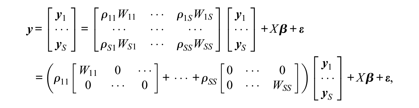
The standard, or first-order, network autocorrelation model in equation (1) is limited to a single network autocorrelation parameter $\rho$ and a single connectivity matrix $W$ . Hence, in this model the network influence is assumed to be homogeneously distributed across the network on the basis of a single influence mechanism. Extending the first-order model to higher-order network autocorrelation models allows a richer dependence structure by including multiple connectivity matrices, representing different influence mechanisms (e.g., geographic adjacency and social similarity). ² This amounts to the functional form

$$\mathit{y}=\sum _{r=1}^R{\rho }_r{W}_r\mathit{y}+X\mathbf{\beta }+\mathbf{\epsilon },\mathbf{\epsilon }~N(0_g,{\sigma }^2{I}_g),$$

(3)

where ${\left\{W_r\right\}}_r$ are distinct connectivity matrices, and the corresponding network autocorrelation parameters ${\left\{{\rho }_r\right\}}_r$ denote the strength of the different influence mechanisms.

In practice, there can be overlap between connectivity matrices; that is, different connectivity matrices may share common ties. Partially overlapping connectivity matrices do not pose identification problems as long as there is no complete overlap (Elhorst et al. 2012), but overlap does make interpretability of the network autocorrelation parameters more difficult (Elhorst et al. 2012; LeSage and Pace 2011). In particular, partial overlap may result in empirically unlikely negative network autocorrelations (Dittrich et al. 2017a; Elhorst et al. 2012). We analyze the numerical effect of overlapping connectivity matrices on the estimation of and hypothesis tests on $\mathbf{\rho }:=({\rho }_1,...,{\rho }_R)$ in more detail in a simulation study in Section 5.

Higher-order network autocorrelation models not only allow one to consider multiple influence mechanisms, but they also allow researchers to partition a network into several subgroups. In the latter case, possible heterogeneity in network influence strength is included in the model by allowing for different levels of network autocorrelation within and between subgroups for a given influence mechanism (e.g., geographic adjacency). Dividing actors in a network into $S$ subgroups, with sizes $g_1,...,g_S$ and $\sum _{s=1}^S{g}_s=g$ , a model with multiple subgroups can be expressed using the representation in equation (3) by writing

$$\begin{array}{c}\multicolumn{1}{c}{\mathit{y}=\left[\begin{array}{c}{\mathit{y}}_1\hfill \\ \multicolumn{1}{c}{\cdots }\\ \multicolumn{1}{c}{{\mathit{y}}_S}\end{array}\right]=\left[\begin{array}{cccccc}{\rho }_{11}{W}_{11}\hfill & \cdots \hfill & {\rho }_{1S}{W}_{1S}\hfill & \multicolumn{1}{c}{\cdots }& \cdots \hfill & \cdots \hfill \\ \multicolumn{1}{c}{{\rho }_{S1}{W}_{S1}}& \cdots \hfill & {\rho }_{\mathrm{SS}}{W}_{\mathrm{SS}}\hfill \end{array}\right]\left[\begin{array}{c}{\mathit{y}}_1\hfill \\ \multicolumn{1}{c}{\cdots }\\ \multicolumn{1}{c}{{\mathit{y}}_S}\end{array}\right]+X\mathbf{\beta }+\mathbf{\epsilon }}\\ \multicolumn{1}{c}{=\left({\rho }_{11}\left[\begin{array}{ccc}{W}_{11}& 0& \cdots \\ 0& \cdots & 0\end{array}\right]+\cdots +{\rho }_{SS}\left[\begin{array}{ccc}0& \cdots & 0\\ 0& \cdots & W_{SS}\end{array}\right]\right)\left[\begin{array}{c}{y}_1\\ \cdots \\ y_S\end{array}\right]+X\beta +\epsilon ,}\end{array}$$

where ${\mathit{y}}_s$ is a vector of length $g_s$ containing the observations for the $g_s$ actors in the $s$ th subgroup of the network, $W_{\mathrm{ss}\prime }$ is a $(g_s\times g_{s\prime })$ connectivity matrix defining the influence relationships between members of subgroup $s\prime$ and members of subgroup $s$ , and ${\rho }_{\mathrm{ss}\prime }$ is a network autocorrelation parameter representing the strength of the network influence of the actors in subgroup $s\prime$ on the actors in subgroup $s$ . Because the sizes of the $S$ subgroups potentially differ, each $W_{\mathrm{ss}\prime }$ is typically row-standardized separately, which removes scale effects and eases direct comparison between the network autocorrelation parameters (McMillen, Singell, and Waddell 2007).

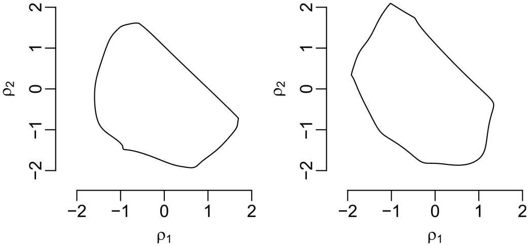
The structure of the likelihood function of higher-order network autocorrelation models remains the same as in the first-order model in equation (2), with $A_{\rho }$ being replaced by $A_{\mathbf{\rho }}:=I_g-\sum _{r=1}^R{\rho }_r{W}_r$ . As in the first-order model, we define the $R$ -dimensional parameter space of $\mathbf{\rho }=({\rho }_1,...,{\rho }_R)$ as the space containing the origin for which $A_{\mathbf{\rho }}$ is nonsingular. Elhorst et al. (2012) provided a simple procedure for checking if a point ${\mathbf{\rho }}^{\ast }\in ℝ$ ^R , given $W_1,...,W_R$ , lies in the corresponding feasible parameter space ${\Theta }_{\mathbf{\rho }}$ . ³ Figure 1 shows two exemplary feasible parameter spaces of $({\rho }_1,{\rho }_2)$ in a second-order network autocorrelation model for simulated data based on nonoverlapping matrices (left) and with 40 percent overlap (right).

Figure 1.

Feasible two-dimensional parameter space ${\Theta }_{({\rho }_1,{\rho }_2)}$ for simulated data based on nonoverlapping connectivity matrices (left) and connectivity matrices with a 40 percent overlap (right).

2.3. Application of a Higher-Order Network Autocorrelation Model: Economic Growth of Labor Productivity

In this subsection, we introduce a data set from the economic growth literature that prompts questions that can readily be answered using the proposed Bayes factor approach. Here, we merely describe the data set and the research questions; in Section 6, we provide solutions to the posed questions.

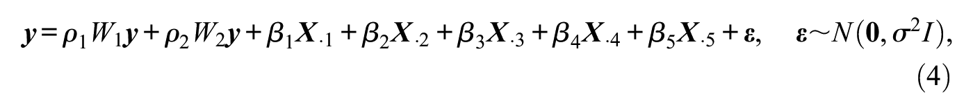
Dall’erba et al. (2009) used a second-order network autocorrelation model to explain the growth rates of labor productivity in the service industry across 188 European regions in 12 countries from 1980 to 2003. To adequately deal with interregional spillovers, the authors introduced two different spatial weight matrices, $W_1$ and $W_2$ , “under the assumption that economic interactions decrease very substantially when a national border is passed” (p. 337). They constructed $W_1$ using a region’s three nearest neighbors within the same country, and $W_2$ was based on the three nearest neighbors in bordering countries. The authors then row-normalized these raw binary connectivity matrices. In addition to an intercept term, Dall’erba et al. (2009) considered four more explanatory variables: the growth rate of market service output in a region, the initial labor productivity gap between the region and the leading region, a measure of the region’s urbanization, and a measure of the region’s accessibility. Thus, their model is given by

$$\mathit{y}={\rho }_1{W}_1\mathit{y}+{\rho }_2{W}_2\mathit{y}+{\beta }_1{\mathit{X}}_{·1}+{\beta }_2{\mathit{X}}_{·2}+{\beta }_3{\mathit{X}}_{·3}+{\beta }_4{\mathit{X}}_{·4}+{\beta }_5{\mathit{X}}_{·5}+\mathbf{\epsilon },\mathbf{\epsilon }~N(0,{\sigma }^{2}I),$$

(4)

where $\mathit{y}\in {\mathbb{R}}^{188}$ is the vector of growth rates of labor productivity in the service industry across the 188 regions, $\mathbf{\beta }\in {\mathbb{R}}^5$ represents the vector of the four regression coefficients plus an intercept term, $X\in {\mathbb{R}}^{188\times 5}$ contains the values for the explanatory variables for the 188 regions, where ${\mathit{X}}_{.i},i\in \{1,...,5\}$ , denotes the $i$ th column of $X$ , $0\in {\mathbb{R}}^{188}$ is a vector of zeros, and $I\in {\mathbb{R}}^{188\times 188}$ represents the corresponding identity matrix.

The authors found that the estimate of ${\rho }_1$ , reflecting interactions within the same country, is positive and statistically significant, indicating the presence of positive spatial within-country spillover effects. On the other hand, the estimate of ${\rho }_2$ is very close to zero and statistically not significant. Dall’erba et al. (2009) concluded by saying that “the results obtained also confirm the hypothesis that economic interactions decrease very substantially when a national border is passed (indeed, the coefficient reflecting external spillovers is not statistically significant)” (p. 342). However, to draw this conclusion, one needs to directly test a corresponding hypothesis, for example, $H_1:{\rho }_1>{\rho }_2=0$ , against a (set of) competing hypothesis (hypotheses), such as $H_0:{\rho }_1={\rho }_2=0$ , $H_2:{\rho }_1>{\rho }_2>0$ , or (and) $H_3:{\rho }_1={\rho }_2>0$ . These four hypotheses correspond to the notion of “no network effects” ( $H_0$ ), “a positive within-country network effect only” ( $H_1$ ), “positive but decreasing network effects after a national border is passed” ( $H_2$ ), and “positive and equally strong within-country and between-country network effects” ( $H_3$ ). Currently, no formal statistical method is available to directly test such hypotheses on multiple network autocorrelations. In the remainder of this article, we develop a Bayesian framework for testing and quantifying the evidence in the data for such hypotheses involving equality as well as order constraints on the network effects. We come back to this empirical example and test these hypotheses against one another using Bayes factors in Section 6. Finally, Dall’erba et al. (2009) stated that “there is evidence that the coefficients in a growth model are potentially varying for different subsets of the total sample” (p. 342). In Section 6, we investigate if there is such evidence in this data set by considering a network autocorrelation model with two subgroups, allowing for differing levels of network autocorrelation within and between the two subgroups.

3. Bayesian Estimation of Higher-Order Network Autocorrelation Models

3.1. Prior Specification

Bayesian estimation starts with formulating prior expectations about the parameters in a model in terms of prior distributions, or priors. These priors summarize the (lack of) information about the model parameters before observing the data. If such prior information is available (e.g., on the basis of previous literature), informative priors for the parameters of interest can be formulated. For the first-order network autocorrelation model, Dittrich et al. (2017a) performed a literature study, looking at the distribution of reported network autocorrelations across many different fields. On the basis of their results, most of the analyzed data in the literature exhibit positive network autocorrelation between 0 and 0.5, and it seems highly unlikely to observe negative network autocorrelation estimates (as previously noted by, e.g., Neuman and Mizruchi 2010). This information could then be used to formulate an informative prior for $\rho$ in a first-order network autocorrelation model, as Dittrich et al. (2017a, 2017b) did. On the other hand, if such prior information is missing, or a researcher deliberately refrains from adding additional information to the model through the prior, noninformative priors are often used (Gelman et al. 2003). In the network autocorrelation model, ${\sigma }^2$ and $\mathbf{\beta }$ are commonly assigned the standard noninformative priors $p\left({\sigma }^2\right)\propto 1/{\sigma }^2$ and $p\left(\mathbf{\beta }\right)\propto 1$ (Hepple 1995a; Holloway, Shankar, and Rahman 2002; LeSage 1997b). These priors assume that all possible values for $\log \left({\sigma }^2\right)$ and $\mathbf{\beta }$ are equally likely a priori. We also do so throughout this article. Note that these priors are not proper in the sense that they do not integrate to a finite value, which does not affect estimation of the model.

We use a general $R$ -variate normal prior for $\mathbf{\rho }$ , $p\left(\mathbf{\rho }\right)={\varphi }_{\mathbf{\mu },\Sigma }\left(\mathbf{\rho }\right){\mathbb{1}}_{{\Theta }_{\mathbf{\rho }}}\left(\mathbf{\rho }\right)c^{-1}$ , where ${\varphi }_{\mathbf{\mu },\Sigma }(·)$ denotes the probability density function of a multivariate normal distribution with prior mean $\mathbf{\mu }$ and prior covariance matrix $\Sigma$ , ${\mathbb{1}}_{·}(·)$ is the standard indicator function, and $c:={\int }_{{\Theta }_{\mathbf{\rho }}}{\varphi }_{\mathbf{\mu },\Sigma }\left(\mathbf{\rho }\right)\mathrm{d}\mathbf{\rho }$ is a normalizing constant representing the probability mass of ${\varphi }_{\mathbf{\mu },\Sigma }(·)$ contained in the network autocorrelation parameters’ space ${\Theta }_{\mathbf{\rho }}$ . If researchers have sufficient prior information about the network autocorrelations, they can specify $\mathbf{\mu }$ and $\Sigma$ directly. Alternatively, when specifying $\Sigma$ vaguely enough, that is, with very large diagonal elements, the prior becomes essentially identical to a proper uniform distribution for $\mathbf{\rho }$ on the bounded parameter space ${\Theta }_{\mathbf{\rho }}$ . ⁴

In summary, we use the following priors for the model parameters, which we assume to be a priori independent from one another:

$$p\left(\mathbf{\rho }\right)={\varphi }_{\mathbf{\mu },\Sigma }\left(\mathbf{\rho }\right){\mathbb{1}}_{{\Theta }_{\mathbf{\rho }}}\left(\mathbf{\rho }\right)c^{-1},$$

(5)

$$p\left({\sigma }^2\right)\propto 1/{\sigma }^2,$$

(6)

$$\begin{array}{cc}\multicolumn{1}{c}{p\left(\mathbf{\beta }\right)}& \propto 1,\hfill \\ \multicolumn{1}{c}{p(\mathbf{\rho },{\sigma }^2,\mathbf{\beta })}& =p\left(\mathbf{\rho }\right)\times p\left({\sigma }^2\right)\times p\left(\mathbf{\beta }\right).\hfill \end{array}$$

(7)

3.2. Posterior Computation

After having specified a prior distribution for the model parameters, the information contained in the observed data $\mathit{y}$ is used to update the prior distribution and to arrive at the posterior distribution, or simply posterior. The posterior is used for all Bayesian inference in the model, for example, to obtain point estimates of model parameters (the posterior mean or the posterior median), to construct Bayesian credible intervals (i.e., intervals in the domain of the posterior), or to determine other statistics of interest, such as the probability that one network effect is stronger than another one for given data, $p({\rho }_1>{\rho }_2|\mathit{y})$ . In this subsection, we specify the posterior in higher-order network autocorrelation models on the basis of the priors from Section 3.1, and we provide an automatic and efficient scheme to sample from this posterior.

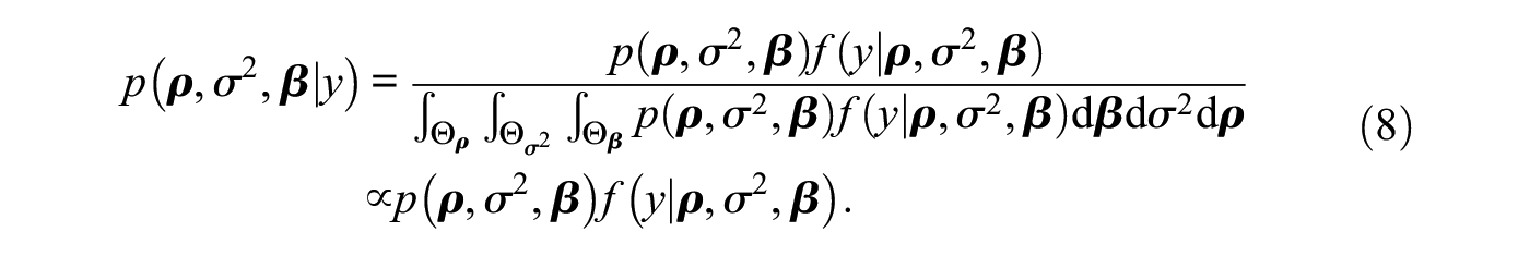
First, Bayes’ theorem gives that the posterior is proportional to the prior multiplied by the likelihood, more precisely

$$\begin{array}{cc}\multicolumn{1}{c}{p(\mathbf{\rho },{\sigma }^2,\mathbf{\beta }|y)}& =\frac{p(\mathbf{\rho },{\sigma }^2,\mathbf{\beta })f(y|\mathbf{\rho },{\sigma }^2,\mathbf{\beta })}{{\int }_{{\Theta }_{\mathbf{\rho }}}{\int }_{{\Theta }_{{\sigma }^2}}{\int }_{{\Theta }_{\mathbf{\beta }}}p(\mathbf{\rho },{\sigma }^2,\mathbf{\beta })f(y|\mathbf{\rho },{\sigma }^2,\mathbf{\beta })\mathrm{d}\mathbf{\beta }\mathrm{d}{\sigma }^2\mathrm{d}\mathbf{\rho }}\hfill \\ \propto p(\mathbf{\rho },{\sigma }^2,\mathbf{\beta })f(y|\mathbf{\rho },{\sigma }^2,\mathbf{\beta }).\hfill \end{array}$$

(8)

The denominator of equation (8) is called the marginal likelihood and ensures that the posterior integrates to unity. The marginal likelihood does not depend on any model parameters and can be ignored in Bayesian estimation of the model. On the other hand, when testing hypotheses, the marginal likelihood does play a central role, as it quantifies how plausible the data are under a specific hypothesis, which we discuss in the following section.

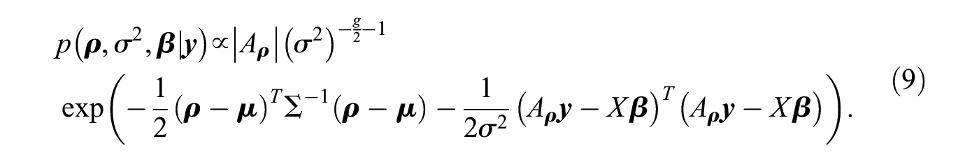
Next, using the priors in equations (5), (6), and (7), and the likelihood function in equation (2), we can express the posterior $p(\mathbf{\rho },{\sigma }^2,\mathbf{\beta }|\mathit{y})$ in higher-order network autocorrelation models as

$$\begin{array}{c}p(\mathbf{\rho },{\sigma }^2,\mathbf{\beta }|\mathit{y})\propto \left|A_{\mathbf{\rho }}\right|{\left({\sigma }^2\right)}^{-\frac{g}{2}-1}\hfill \\ \exp (-\frac{1}{2}{(\mathbf{\rho }-\mathbf{\mu })}^T{\Sigma }^{-1}(\mathbf{\rho }-\mathbf{\mu })-\frac{1}{2{\sigma }^2}{(A_{\mathbf{\rho }}\mathit{y}-X\mathbf{\beta })}^T(A_{\mathbf{\rho }}\mathit{y}-X\mathbf{\beta })).\hfill \end{array}$$

(9)

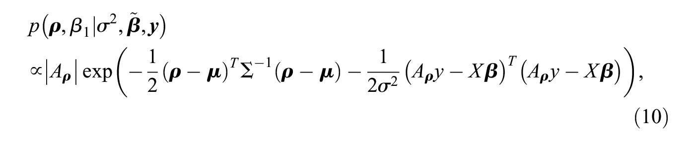
However, the posterior in equation (9) does not belong to a family of known probability distributions, so we cannot directly infer its posterior mean, its quantiles, or other quantities of interest. ⁵ In this case, it is common to sample random draws from the posterior and to use these posterior draws to approximate any desired statistic. An efficient method is to sequentially draw from the conditional posteriors, that is, the posterior of one parameter (block) given the remaining parameters and the data (Gelfand and Smith 1990; Geman and Geman 1984). ⁶ Extending the proposed method for the first-order network autocorrelation model in Dittrich et al. (2017a) to higher-order models, we sample the model parameters according to the following blocks: $(\mathbf{\rho },{\beta }_1),{\sigma }^2$ , and $\tilde{\beta }$ , where ${\beta }_1$ denotes the model’s intercept and $\tilde{\beta }:=({\beta }_2,...,{\beta }_k)$ contains the remaining regression coefficients. By simultaneously sampling $\mathbf{\rho }$ and ${\beta }_1$ , we can better capture potential posterior correlation between the network effects as well as potential correlation between the network effects and the intercept (Dittrich et al. 2017a). The conditional posteriors for the proposed blocks are then given by (see, e.g., LeSage 1997a)

$$\begin{array}{c}p(\mathbf{\rho },{\beta }_1|{\sigma }^2,\tilde{\beta },\mathit{y})\hfill \\ \propto \left|A_{\mathbf{\rho }}\right|\exp (-\frac{1}{2}{(\mathbf{\rho }-\mathbf{\mu })}^T{\Sigma }^{-1}(\mathbf{\rho }-\mathbf{\mu })-\frac{1}{2{\sigma }^2}{(A_{\mathbf{\rho }}y-X\mathbf{\beta })}^T(A_{\mathbf{\rho }}y-X\mathbf{\beta })),\hfill \end{array}$$

(10)

$$p({\sigma }^2|\mathbf{\rho },{\beta }_1,\tilde{\beta },\mathit{y})~\mathrm{IG}(\frac{g}{2},\frac{{(A_{\mathbf{\rho }}\mathit{y}-X\mathbf{\beta })}^T(A_{\mathbf{\rho }}\mathit{y}-X\mathbf{\beta })}{2}),$$

(11)

$$p(\tilde{\beta }|\mathbf{\rho },{\beta }_1,{\sigma }^2,\mathit{y})~N({\mathbf{\mu }}_{\tilde{\beta }},{\Sigma }_{\tilde{\beta }}),$$

(12)

where $\mathrm{IG}(·,·)$ denotes the inverse gamma distribution, and ${\mathbf{\mu }}_{\tilde{\beta }}$ and ${\Sigma }_{\tilde{\beta }}$ are given in Appendix A.

Drawing from the conditional posteriors in equations (11) and (12) can be done using standard statistical software. In contrast, the conditional posterior in equation (10) does not have a well-known form and cannot be directly sampled from. Instead, we use the Metropolis-Hastings algorithm (Hastings 1970; Metropolis et al. 1953) to generate draws from the conditional posterior for $(\mathbf{\rho },{\beta }_1)$ . In short, the algorithm generates candidate values for the conditional posterior from a candidate-generating distribution that can be easily sampled from and subsequently accepts, or rejects, the draws with a certain probability. The algorithm’s efficiency mainly depends on the shape of the proposed candidate-generating distribution; if possible, exploiting the form of the conditional posterior and specifying a candidate-generating distribution that closely approximates it results in efficient solutions (Chib and Greenberg 1994, 1995, 1998).

We first approximate $\log \left(\left|A_{\mathbf{\rho }}\right|\right)$ by a quadratic polynomial in $\mathbf{\rho }$ by virtue of Jacobi’s formula and the Mercator series (see Appendix A). Next, we observe that the logarithm of the exponential in equation (10) can also be written as a quadratic polynomial in $(\mathbf{\rho },{\beta }_1)$ . Hence, the logarithm of the conditional posterior itself can be approximated by a quadratic polynomial in $(\mathbf{\rho },{\beta }_1)$ . Finally, by equating coefficients of this quadratic polynomial with the log-kernel of the probability density function of an $(R+1)$ -variate normal distribution, the density in equation (10) can be approximated by an $(R+1)$ -variate normal candidate-generating density for $(\mathbf{\rho },{\beta }_1)$ that is tailored to the conditional posterior for $(\mathbf{\rho },{\beta }_1)$ . ⁷ All details and the full sampling scheme can be found in Appendix A.

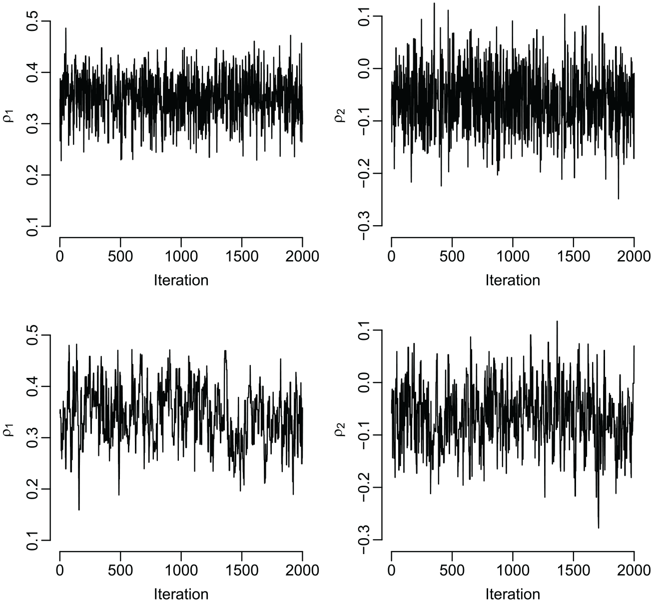
We implemented our proposed approach in R (R Core Team 2017) and compared its performance with a sampling scheme that does not block the network autocorrelation parameters and the intercept but uses one-dimensional random walk algorithms to generate draws for each network effect sequentially, as in Zhang et al. (2013). Figure 2 shows exemplary trace plots of posterior draws for ${\rho }_1$ and ${\rho }_2$ on the basis of the two sampling schemes and the data in Dall’erba et al. (2009) with model (4). We see that our method results in a more efficient implementation than drawing each network effect separately, as it generates Markov chains that explore the corresponding parameter space of $({\rho }_1,{\rho }_2)$ much faster. Finally, our approach is fully automatic in the sense that there are no parameters to be tuned in the Metropolis-Hastings algorithm, such as the variance of candidate-generating distributions.

Figure 2.

Trace plots of posterior draws for ${\rho }_1$ and ${\rho }_2$ on the basis of our proposed scheme (top row) and a random walk algorithm (bottom row) for the data in Dall’erba et al. (2009) with model (4).

To conclude, the presented sampling algorithm allows researchers to automatically and efficiently draw from the posterior on the basis of a general multivariate normal prior for the network autocorrelation parameters, including informative as well as noninformative specifications. Such efficient sampling is essential for performing any Bayesian estimation of the model, which solely relies on the generated posterior draws. An R program that implements our scheme is available at https://github.com/DittrichD/BayesNAM.

4. Bayesian Hypothesis Testing in Higher-Order Network Autocorrelation Models

In many network studies, researchers have competing theories about the specific order of different network effect strengths. These theories can be formulated as hypotheses on the network autocorrelation parameters, for example, as $H_1:{\rho }_1>{\rho }_2=0$ , $H_2:{\rho }_1>{\rho }_2>0$ , or $H_3:{\rho }_1={\rho }_2>0$ , and can include as many network autocorrelation parameters as relevant to one’s theory. The focus of interest then lies on which substantive theory, or hypothesis, is most plausible and most supported by the data and how strongly. In this section, we consider $T\ge 2$ constrained hypotheses on the network effects, where a hypothesis $H_t$ , $t\in \{0,...,T-1\}$ , contains $q_t^E$ equality and $q_t^I$ inequality constraints on $\mathbf{\rho }$ , that is,

$$H_t:=\{\begin{array}{c}{R}_t^E\mathbf{\rho }=r_t^E\hfill \\ \multicolumn{1}{c}{R_t^I\mathbf{\rho }>r_t^I,}\end{array}$$

(13)

where $R_t^E$ and $r_t^E$ are a $(q_t^E\times R)$ matrix and a vector of length $R$ , respectively, containing the coefficients of the $q_t^E$ equality constraints under hypothesis $H_t$ . Equivalently, the $(q_t^I\times R)$ matrix $R_t^I$ and the vector $r_t^I$ contain the coefficients of the $q_t^I$ inequality constraints. For example, the constraints induced by the three hypotheses $H_1:{\rho }_1>{\rho }_2=0$ , $H_2:{\rho }_1>{\rho }_2>0$ , and $H_3:{\rho }_1={\rho }_2>0$ can be represented by equation (13) as ⁸

$$H_1:R_1^E=(0,1),r_1^E=0,R_1^I=(1,0),r_1^I=0,$$

$$H_2:R_2^I=\left(\begin{array}{cc}1\hfill & -1\hfill \\ \multicolumn{1}{c}{0}& 1\hfill \end{array}\right),{\mathit{r}}_2^I=(0,0),$$

$$H_3:R_3^E=(1,-1),r_3^E=0,R_3^I=(1,0),r_3^I=0.$$

Bayes factors for testing hypotheses of the form in equation (13) have also been proposed for other types of parameters, such as group variances (Böing-Messing et al. 2017), intraclass correlations (Mulder and Fox 2018), and regression effects (Mulder, Hoijtink, and Klugkist 2010).

4.1. The Bayes Factor

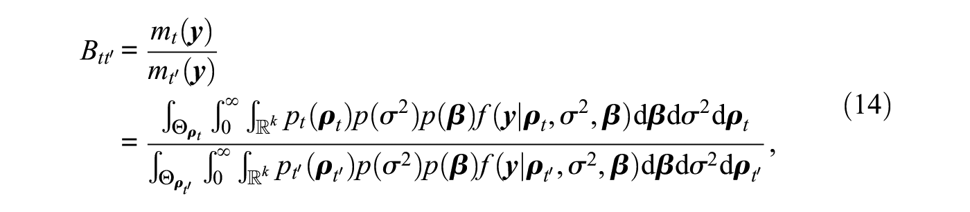
The Bayes factor is a comparative Bayesian hypothesis testing criterion that directly quantifies the relative evidence in the data in favor of a hypothesis. The Bayes factor of hypothesis $H_t$ against hypothesis $H_{t\prime }$ , $t,t\prime \in \{0,...,T-1\}$ , is defined as the ratio of the marginal likelihoods under the two hypotheses, that is, in the network autocorrelation model as

$$\begin{array}{c}\multicolumn{1}{c}{B_{\mathrm{tt}\prime }=\frac{m_t\left(\mathit{y}\right)}{m_{t\prime }\left(\mathit{y}\right)}}\\ \multicolumn{1}{c}{=\frac{{\int }_{{\Theta }_{{\mathbf{\rho }}_t}}{\int }_0^{\infty }{\int }_{{\mathbb{R}}^k}{p}_t\left({\mathbf{\rho }}_t\right)p\left({\sigma }^2\right)p\left(\mathbf{\beta }\right)f(\mathit{y}|{\mathbf{\rho }}_t,{\sigma }^2,\mathbf{\beta })\mathrm{d}\mathbf{\beta }\mathrm{d}{\sigma }^2\mathrm{d}{\mathbf{\rho }}_t}{{\int }_{{\Theta }_{{\mathbf{\rho }}_{t\prime }}}{\int }_0^{\infty }{\int }_{{\mathbb{R}}^k}{p}_{t\prime }\left({\mathbf{\rho }}_{t\prime }\right)p\left({\sigma }^2\right)p\left(\mathbf{\beta }\right)f(\mathit{y}|{\mathbf{\rho }}_{t\prime },{\sigma }^2,\mathbf{\beta })\mathrm{d}\mathbf{\beta }\mathrm{d}{\sigma }^2\mathrm{d}{\mathbf{\rho }}_{t\prime }},}\end{array}$$

(14)

where ${\mathbf{\rho }}_t$ are the network autocorrelation parameters under hypothesis $H_t$ , $p_t\left({\mathbf{\rho }}_t\right)$ denotes their prior density, and ${\Theta }_{{\mathbf{\rho }}_t}$ is the corresponding parameter space (Kass and Raftery 1995). We assume common priors for ${\sigma }^2$ and $\mathbf{\beta }$ under both hypothesis $H_t$ and hypothesis $H_{t\prime }$ as they are seen as nuisance parameters in the presented framework. The exact form of the priors for these nuisance parameters typically does not alter the magnitude of the Bayes factor (Kass and Raftery 1995).

The marginal likelihood under hypothesis $H_t$ , $m_t\left(\mathit{y}\right)$ , is a weighted average likelihood over the parameter space under hypothesis $H_t$ , with the prior $p_t\left({\mathbf{\rho }}_t\right)$ under hypothesis $H_t$ acting as a weight function. Therefore, it can be interpreted as the probability that the data were observed under hypothesis $H_t$ . Hence, the Bayes factor, as the ratio of two marginal likelihoods, quantifies the relative evidence that the data were observed under hypothesis $H_t$ rather than hypothesis $H_{t\prime }$ . For example, when $B_{\mathrm{tt}\prime }=5$ , this indicates that the data are five times more likely to have occurred under hypothesis $H_t$ compared with hypothesis $H_{t\prime }$ . Conversely, when $B_{\mathrm{tt}\prime }=1/5$ , it is five times more likely to have observed the data under hypothesis $H_{t\prime }$ than under hypothesis $H_t$ .

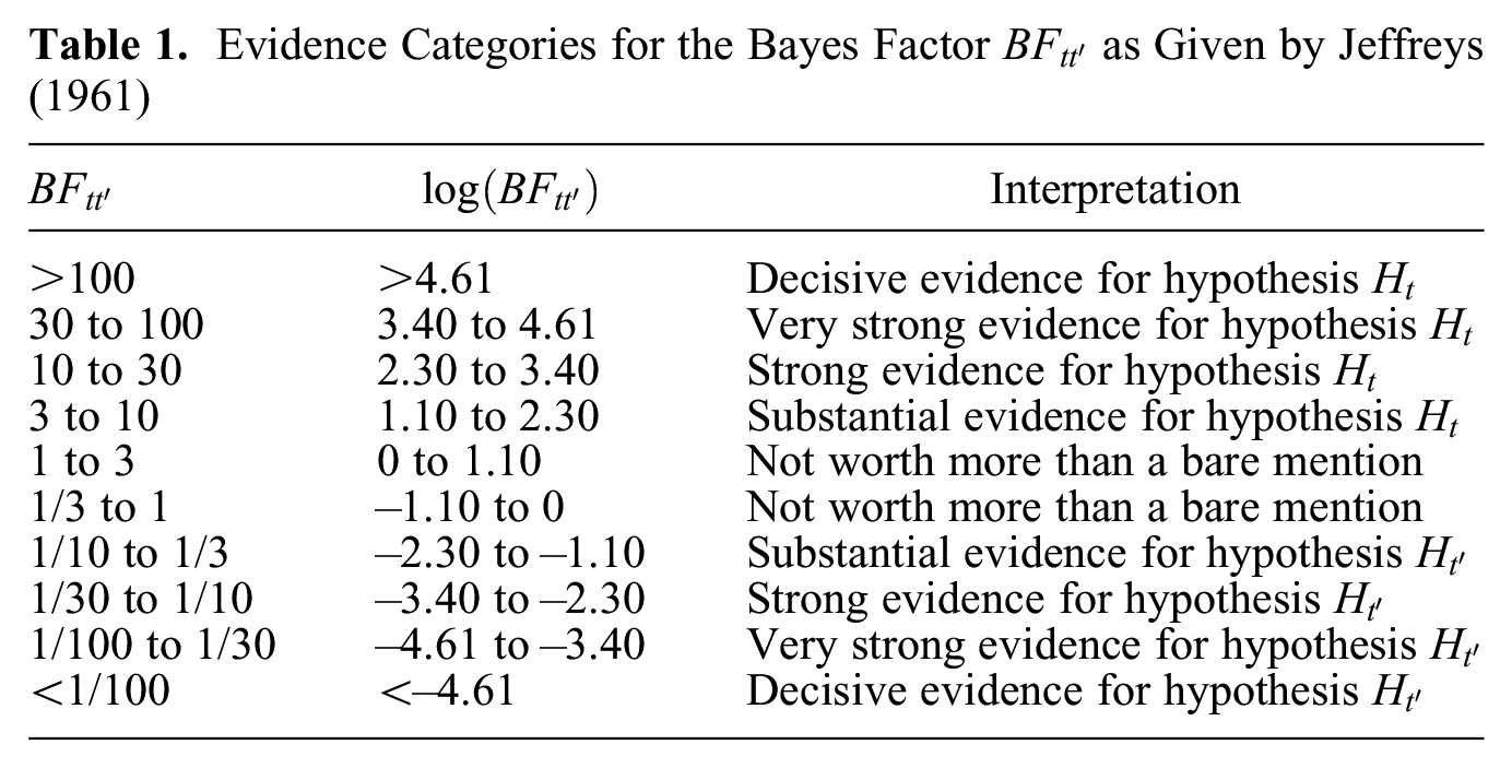
To facilitate interpretation of the Bayes factor, Jeffreys (1961) proposed a classification scheme that groups Bayes factors into different categories (see Table 1). For example, there is “strong” evidence in the data for hypothesis $H_t$ , relative to hypothesis $H_{t\prime }$ , when $B_{\mathrm{tt}\prime }>10$ and, equivalently, “strong” relative evidence in the data for hypothesis $H_{t\prime }$ when $B_{\mathrm{tt}\prime }<1/10$ . This grouping provides verbal descriptions and rules of thumb when speaking of relative evidence in the data in favor of a hypothesis, but it is still somewhat arbitrary. Ultimately, the interpretation of the magnitude of a Bayes factor should hinge on the context of the research question (Kass and Raftery 1995). For some introductory texts on Bayes factor testing in social science research, we refer the interested reader to Braeken et al. (2015), Raftery (1995), van de Schoot et al. (2011), or Wagenmakers (2007).

Table 1.

Evidence Categories for the Bayes Factor $B{F}_{\mathrm{tt}\prime }$ as Given by Jeffreys (1961)

$B{F}_{\mathrm{tt}\prime }$	$\log \left(B{F}_{\mathrm{tt}\prime }\right)$	Interpretation
>100	>4.61	Decisive evidence for hypothesis $H_t$
30 to 100	3.40 to 4.61	Very strong evidence for hypothesis $H_t$
10 to 30	2.30 to 3.40	Strong evidence for hypothesis $H_t$
3 to 10	1.10 to 2.30	Substantial evidence for hypothesis $H_t$
1 to 3	0 to 1.10	Not worth more than a bare mention
1/3 to 1	−1.10 to 0	Not worth more than a bare mention
1/10 to 1/3	−2.30 to −1.10	Substantial evidence for hypothesis $H_{t\prime }$
1/30 to 1/10	−3.40 to −2.30	Strong evidence for hypothesis $H_{t\prime }$
1/100 to 1/30	−4.61 to −3.40	Very strong evidence for hypothesis $H_{t\prime }$
<1/100	<–4.61	Decisive evidence for hypothesis $H_{t\prime }$

4.2. Bayes Factor Computation

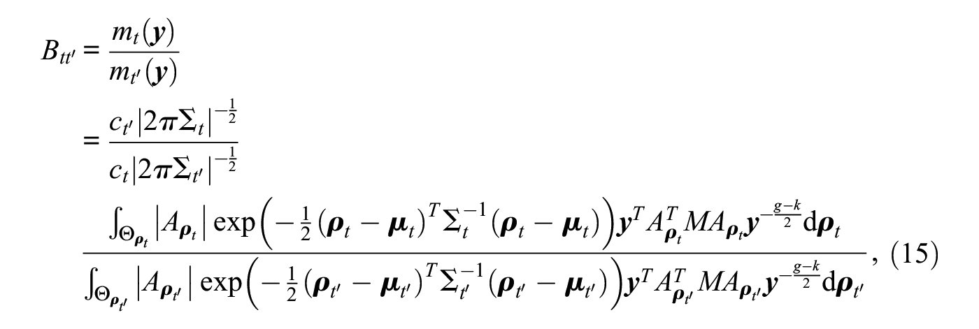
In this section, we present efficient methods to compute marginal likelihoods and Bayes factors in higher-order network autocorrelation models. Using a multivariate normal prior for ${\mathbf{\rho }}_t$ under hypothesis $H_t$ , $p_t\left({\mathbf{\rho }}_t\right)={\varphi }_{{\mathbf{\mu }}_t,{\Sigma }_t}\left({\mathbf{\rho }}_t\right){\mathbb{1}}_{{\Theta }_{{\mathbf{\rho }}_t}}\left({\mathbf{\rho }}_t\right)c_t^{-1}$ , $c_t:={\int }_{{\Theta }_{{\mathbf{\rho }}_t}}{\varphi }_{{\mathbf{\mu }}_t,{\Sigma }_t}\left({\mathbf{\rho }}_t\right)\mathrm{d}{\mathbf{\rho }}_t$ , the noninformative prior $p({\sigma }^2,\mathbf{\beta })\propto 1/{\sigma }^2$ for the nuisance parameters ${\sigma }^2$ and $\mathbf{\beta }$ , and after analytically integrating out ${\sigma }^2$ and $\mathbf{\beta }$ , the Bayes factor of hypothesis $H_t$ against hypothesis $H_{t\prime }$ in equation (14) reduces to

$$\begin{array}{c}\multicolumn{1}{c}{B_{\mathrm{tt}\prime }=\frac{m_t\left(\mathit{y}\right)}{m_{t\prime }\left(\mathit{y}\right)}}\\ \multicolumn{1}{c}{=\frac{c_{t\prime }{\left|2\pi {\Sigma }_t\right|}^{-\frac{1}{2}}}{c_t{\left|2\pi {\Sigma }_{t\prime }\right|}^{-\frac{1}{2}}}}\\ \multicolumn{1}{c}{\frac{{\int }_{{\Theta }_{{\mathbf{\rho }}_t}}\left|A_{{\mathbf{\rho }}_t}\right|\exp (-\frac{1}{2}{({\mathbf{\rho }}_t-{\mathbf{\mu }}_t)}^T{\Sigma }_t^{-1}({\mathbf{\rho }}_t-{\mathbf{\mu }}_t)){\mathit{y}}^T{A}_{{\mathbf{\rho }}_t}^{T}M{A}_{{\mathbf{\rho }}_t}{\mathit{y}}^{-\frac{g-k}{2}}\mathrm{d}{\mathbf{\rho }}_t}{{\int }_{{\Theta }_{{\mathbf{\rho }}_{t\prime }}}\left|A_{{\mathbf{\rho }}_{t\prime }}\right|\exp (-\frac{1}{2}{({\mathbf{\rho }}_{t\prime }-{\mathbf{\mu }}_{t\prime })}^T{\Sigma }_{t\prime }^{-1}({\mathbf{\rho }}_{t\prime }-{\mathbf{\mu }}_{t\prime })){\mathit{y}}^T{A}_{{\mathbf{\rho }}_{t\prime }}^{T}M{A}_{{\mathbf{\rho }}_{t\prime }}{\mathit{y}}^{-\frac{g-k}{2}}\mathrm{d}{\mathbf{\rho }}_{t\prime }},}\end{array}(15)$$

(15)

where $M:=I_g-X{\left(X^{T}X\right)}^{-1}{X}^T$ . ⁹

The normalizing constants $c_t$ and $c_{t\prime }$ in equation (15) correspond to the prior probabilities that the unconstrained priors for ${\mathbf{\rho }}_t$ under hypothesis $H_t$ and for ${\mathbf{\rho }}_{t\prime }$ under hypothesis $H_{t\prime }$ , $N({\mathbf{\mu }}_{\mathit{t}},{\Sigma }_t)$ and $N({\mathbf{\mu }}_{t\prime },{\Sigma }_{t\prime })$ , are in agreement with the constraints imposed under the two hypotheses. They can be approximated by simple rejection sampling, that is, by sampling draws from the unconstrained priors and recording the proportions of draws that are in agreement with the constraints. The remaining integrals in the numerator and denominator of equation (15) do not have closed-form solutions and have to be evaluated numerically. For this purpose, we rely on an importance sampling procedure (Owen and Zhou 2000) that is explained next.

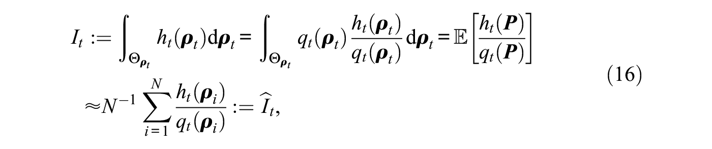
Let $h_t\left({\mathbf{\rho }}_t\right):=\left|A_{{\mathbf{\rho }}_t}\right|\exp (-\frac{1}{2}{({\mathbf{\rho }}_t-{\mathbf{\mu }}_t)}^T{\Sigma }_t^{-1}({\mathbf{\rho }}_t-{\mathbf{\mu }}_t)){\mathit{y}}^T{A}_{{\mathbf{\rho }}_t}^{T}M{A}_{{\mathbf{\rho }}_t}{\mathit{y}}^{-\frac{g-k}{2}}$ denote the integrand in the numerator of equation (15) (all steps apply equivalently to $h_{t\prime }\left({\mathbf{\rho }}_{t\prime }\right)$ ). Then, we can write for the numerator of equation (15)

$$\begin{array}{c}\multicolumn{1}{c}{I_t:={\int }_{{\Theta }_{{\mathbf{\rho }}_t}}{h}_t\left({\mathbf{\rho }}_t\right)\mathrm{d}{\mathbf{\rho }}_t={\int }_{{\Theta }_{{\mathbf{\rho }}_t}}{q}_t\left({\mathbf{\rho }}_t\right)\frac{h_t\left({\mathbf{\rho }}_t\right)}{q_t\left({\mathbf{\rho }}_t\right)}\mathrm{d}{\mathbf{\rho }}_t=\mathbb{E}\left[\frac{h_t\left(\mathit{P}\right)}{q_t\left(\mathit{P}\right)}\right]}\\ \multicolumn{1}{c}{\approx N^{-1}\sum _{i=1}^N\frac{h_t\left({\mathbf{\rho }}_i\right)}{q_t\left({\mathbf{\rho }}_i\right)}:={\hat{I}}_t,}\end{array}$$

(16)

where $\mathit{P}$ is a random variable with probability density function $q_t(·)$ known as the importance density, $\mathbb{E}[h_t\left(\mathit{P}\right)/q_t\left(\mathit{P}\right)]$ denotes the expected value for $h_t\left(\mathit{P}\right)/q_t\left(\mathit{P}\right)$ , and ${\mathbf{\rho }}_i$ are draws from $q_t(·)$ , forming realizations of $\mathit{P}$ . The specification of the importance density is crucial for the algorithm’s efficiency, where we aim to construct a density that closely follows the actual integrand but has heavier tails than the latter and is easy to sample from (Owen and Zhou 2000).

As in Section 3.2, we approximate $\log (|A_{{\mathbf{\rho }}_t}|)$ by a second-order polynomial in ${\mathbf{\rho }}_t$ at its maximum, the origin. This results in a normal approximation of $\left|A_{{\mathbf{\rho }}_t}\right|$ . We apply the same rationale to the third term in $h_t\left({\mathbf{\rho }}_t\right)$ , ${\mathit{y}}^T{A}_{{\mathbf{\rho }}_t}^{T}M{A}_{{\mathbf{\rho }}_t}{\mathit{y}}^{-(g-k)/2}$ . Hence, $h_t\left({\mathbf{\rho }}_t\right)$ can be approximated by the product of three multivariate normal densities that itself is a multivariate normal density, which we use as importance density in equation (16). ¹⁰ Finally, as ${\mathbf{\rho }}_t$ approaches the boundary of ${\Theta }_{{\mathbf{\rho }}_t}$ , the proposed normal importance density has heavier tails than $h_t\left({\mathbf{\rho }}_t\right)$ , because in this case $\left|A_{{\mathbf{\rho }}_t}\right|$ decreases toward zero, but the normal importance density does not. This ensures a finite variance of the importance sampling estimate ${\hat{I}}_t$ and reliable estimation of the associated Bayes factors. All details can be found in Appendix B.

4.3. A Default Prior for $\rho$

When testing multiple hypotheses against one another, a prior for the tested model parameters has to be specified under each hypothesis. Arguably, eliciting a prior under each hypothesis directly can become difficult and cumbersome, especially with a large number of hypotheses at hand. As an alternative, we propose an automatic empirical Bayes procedure (Carlin and Louis 2000) for constructing a default prior $p_t\left({\mathbf{\rho }}_t\right)$ under each hypothesis $H_t$ such that the marginal likelihood under every hypothesis $H_t$ is maximized.

First, we center the multivariate normal default prior $p_t\left({\mathbf{\rho }}_t\right)$ under hypothesis $H_t$ around the origin. The motivation for this choice is that the origin is located at the boundary of typical (in)equality constrained hypotheses in the network autocorrelation model, such as $H_1:{\rho }_1>{\rho }_2=0$ , $H_2:{\rho }_1>{\rho }_2>0$ , or $H_3:{\rho }_1={\rho }_2>0$ , and previous literature on order constrained hypothesis testing suggests “there is a gain of evidence for the inequality constrained hypothesis that is supported by the data when the unconstrained prior is located on the boundary” (Mulder 2014:452). Second, in contrast to Bayesian estimation, assigning very large values to the diagonal elements of the prior’s covariance matrix ${\Sigma }_t$ is not feasible in hypothesis testing. In hypothesis testing, we need to explicitly calculate the normalizing constant $c_t={\int }_{{\Theta }_{{\mathbf{\rho }}_t}}{\varphi }_{{\mathbf{\mu }}_t,{\Sigma }_t}\left({\mathbf{\rho }}_t\right)\mathrm{d}{\mathbf{\rho }}_t$ , and a vague formulation of ${\Sigma }_t$ makes this computation either unstable or tremendously time consuming because of the fairly small parameter space ${\Theta }_{{\mathbf{\rho }}_t}$ . ¹¹ Instead, we set the prior covariance matrix ${\Sigma }_t$ of the free network autocorrelation parameter(s) under a hypothesis, for example, ${\rho }_1$ under hypothesis $H_1:{\rho }_1>{\rho }_2=0$ , to the product of the corresponding asymptotic variance-covariance matrix of the maximum likelihood estimate of ${\mathbf{\rho }}_t$ and a hypothesis-specific scaling factor ${\sigma }_t^2$ , similar to Zellner’s g-prior (Zellner 1986). In mathematical notation, ${\Sigma }_t={\sigma }_t^{2}I{\left({\mathbf{\rho }}_t\right)}^{-1}$ , where $I\left({\mathbf{\rho }}_t\right)$ denotes the submatrix of the network autocorrelation model’s Fisher information matrix $I({\mathbf{\rho }}_t,{\sigma }^2,\mathbf{\beta })$ . Hence, there is only one free parameter in the prior specification of ${\Sigma }_t$ left, ${\sigma }_t^2$ . Following Hansen and Yu (2001) and Liang et al. (2008), we use a local empirical Bayes approach and choose ${\sigma }_t^2$ such that the associated marginal likelihood $m_t\left(\mathit{y}\right)$ is maximized, avoiding arbitrary prior specification. Because there is no analytic solution to this maximization problem, one way to approximate the maximum of $m_t\left(\mathit{y}\right)$ is to compute the marginal likelihood on a grid of increasing values for ${\sigma }_t^2$ until a stopping rule is reached, for example, until the marginal likelihood is not increasing anymore, or until it is not increasing by more than some tolerance factor. ¹²

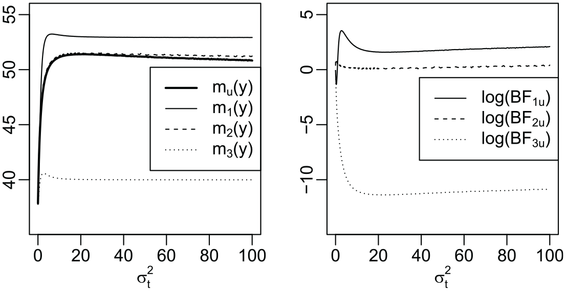
Figure 3 shows the marginal likelihoods under the three constrained hypotheses $H_1:{\rho }_1>{\rho }_2=0$ , $H_2:{\rho }_1>{\rho }_2>0$ , and $H_3:{\rho }_1={\rho }_2>0$ ; the marginal likelihood under an unconstrained hypothesis $H_u:({\rho }_1,{\rho }_2)\in {\Theta }_{({\rho }_1,{\rho }_2)}$ ; and the logarithm of the Bayes factors of the three constrained hypotheses against the unconstrained hypothesis $H_u$ as a function of ${\sigma }_t^2$ , $t\in \{1,2,3,u\}$ , for the data in Dall’erba et al. (2009) with model (4). All of the marginal likelihoods sharply increase for smaller values for ${\sigma }_t^2$ before they gradually decrease after having reached their respective maxima. The associated Bayes factors, in which we are ultimately interested, appear fairly robust to the choice of ${\sigma }_t^2$ , except for extremely small values for ${\sigma }_t^2$ . For the vast majority of data sets we looked at, we observed essentially the same pattern, with almost all the optimal values for ${\sigma }_t^2$ lying between 2 and 10.

Figure 3.

Marginal likelihoods $m_t\left(\mathit{y}\right)$ , $t\in \{1,2,3,u\}$ , under the hypotheses $H_1:{\rho }_1>{\rho }_2=0$ , $H_2:{\rho }_1>{\rho }_2>0$ , $H_3:{\rho }_1={\rho }_2>0$ , and $H_u:({\rho }_1,{\rho }_2)\in {\Theta }_{({\rho }_1,{\rho }_2)}$ as a function of ${\sigma }_t^2$ (left), and the logarithm of the Bayes factors $\log \left(B{F}_{1u}\right),\log \left(B{F}_{2u}\right),$ and $\log \left(B{F}_{3u}\right)$ as a function of ${\sigma }_t^2$ (right) for the data in Dall’erba et al. (2009) with model (4).

In summary, we showed how Bayes factors can be used to quantify the evidence in the data for hypotheses with order constraints on the network autocorrelation parameters. In addition, we provided methodology to efficiently compute such Bayes factors without any need to subjectively elicit priors for the network effects. This ultimately allows network scholars to test and verify any kind of expectations they have about the strength of different network effects. An R program that implements our methodology will be available at https://github.com/DittrichD/BayesNAM.

5. Simulation Study

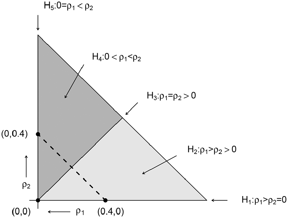
We performed a simulation study to investigate the performance of the proposed Bayesian estimator and Bayes factors in a second-order network autocorrelation model. First, we compared the Bayesian estimator from Section 3.2 with the maximum likelihood estimator in terms of bias of the network effects and frequentist coverage of the corresponding credible and confidence intervals. Here, we use the term coverage to indicate the proportion of times in which the true, that is, data-generating, network effects were contained in the credible and confidence intervals. Second, because researchers are generally interested in testing whether (some) network effects are zero or whether one network effect is larger than another, we considered a multiple hypothesis test with the following five hypotheses: $H_1:{\rho }_1>{\rho }_2=0$ , $H_2:{\rho }_1>{\rho }_2>0$ , $H_3:{\rho }_1={\rho }_2>0$ , $H_4:0<{\rho }_1<{\rho }_2$ , and $H_5:0={\rho }_1<{\rho }_2$ . We investigated if and how fast the different Bayes factors converge to a true data-generating hypothesis and how robust these findings are to various degrees of overlap between two connectivity matrices.

5.1. Study Design

In our simulation study, we generated data $\mathit{y}$ via $\mathit{y}=A_{({\rho }_1,{\rho }_2)}^{-1}(X\mathbf{\beta }+\mathbf{\epsilon }),\mathbf{\epsilon }~N(0_g,I_g)$ , for four network sizes $g$ ( $g\in \{50,100,200,400\}$ ), three levels of overlap between $W_1$ and $W_2$ (0 percent, 20 percent, and 40 percent), and both $W_1$ and $W_2$ having an average degree of four. We simulated random nonsymmetric binary connectivity matrices using the rgraph() function from the sna package in R (Butts 2008), randomly rearranged ties when accounting for overlap, and subsequently row-standardized the raw connectivity matrices. Furthermore, we drew independent values from a standard normal distribution for the elements of $X\in {\mathbb{R}}^{g\times 4}$ (excluding the first column which is a vector of ones), $\mathbf{\beta }\in {\mathbb{R}}^4$ , and $\mathbf{\epsilon }\in {\mathbb{R}}^g$ .

In our first experiment, we set the two network effects to $({\rho }_1,{\rho }_2)=(0.2,0.2)$ and simulated 1,000 data sets for each of the 12 scenarios (four network sizes × three levels of overlap × one network effects size). ¹³ For the Bayesian estimator, we used the standard improper prior $p({\sigma }^2,\mathbf{\beta })\propto 1/{\sigma }^2$ for the nuisance parameters and a noninformative bivariate normal prior for $({\rho }_1,{\rho }_2)$ , $p({\rho }_1,{\rho }_2)\propto N(0_2,100\times I_2)$ , which essentially corresponds to a uniform prior for $({\rho }_1,{\rho }_2)\in {\Theta }_{({\rho }_1,{\rho }_2)}$ . We drew 1,000 realizations from the resulting posteriors relying on the methods described in Section 3.2, taking the maximum likelihood estimate of $(({\rho }_1,{\rho }_2),{\sigma }^2,\mathbf{\beta })$ as the starting value in the sampling algorithm (see Appendix A). We used the marginal posterior median as point estimator and the 95 percent equal-tailed credible interval for coverage analysis. We obtained the maximum likelihood estimates as well as their standard errors and associated asymptotic confidence intervals applying the lnam() function from the sna package in R.

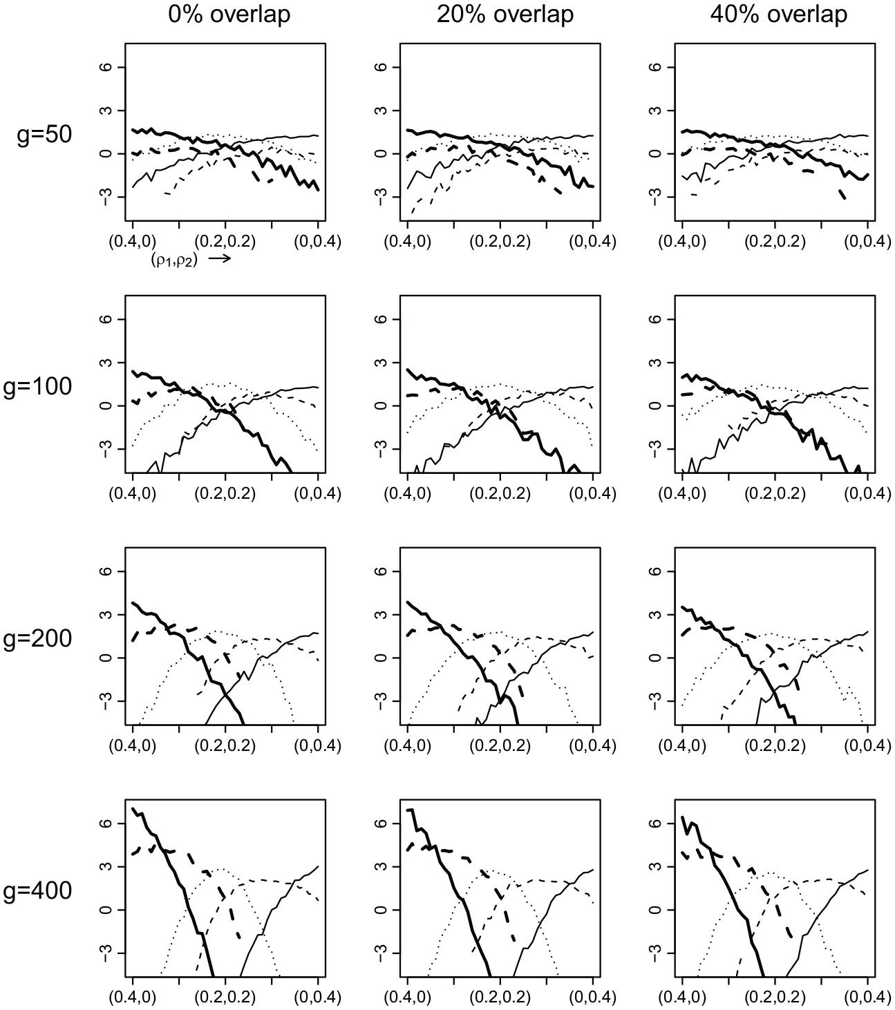
In our second experiment, we considered 41 network effects sizes $({\rho }_1,{\rho }_2)$ ( $({\rho }_1,{\rho }_2)$ $\in \{(0.40,0),(0.39,0.01),\dots ,(0,0.40)\}$ ) and simulated 100 data sets for each of the 492 scenarios (four network sizes × three levels of overlap × 41 network effects sizes). Figure 4 shows the trajectory of the network effects and depicts the five tested hypotheses, $H_1:{\rho }_1>{\rho }_2=0$ , $H_2:{\rho }_1>{\rho }_2>0$ , $H_3:{\rho }_1={\rho }_2>0$ , $H_4:0<{\rho }_1<{\rho }_2$ , and $H_5:0={\rho }_1<{\rho }_2$ . We specified the prior under each of the five hypotheses on the basis of the proposed empirical Bayes procedure in Section 4.3. ¹⁴ To compute the normalizing constants $c_2$ and $c_4$ , we generated draws from the unconstrained bivariate normal prior for $({\rho }_1,{\rho }_2)$ until we obtained 1,000 draws in agreement with the constraints imposed under hypothesis $H_2$ and hypothesis $H_4$ , respectively. Then, we approximated the normalizing constants by the reciprocals of the proportion of the total number of draws in agreement with the constraints. For the hypotheses with only one free network autocorrelation parameter, that is, $H_1:{\rho }_1>{\rho }_2=0$ , $H_3:{\rho }_1={\rho }_2>0$ , and $H_5:0={\rho }_1<{\rho }_2$ , we directly obtained the corresponding normalizing constants by using the pnorm() function in R, as the bounds of the feasible range of a single free network autocorrelation parameter are known exactly (see Section 2.1). Finally, for all hypotheses we drew 1,000 realizations from their (unconstrained) importance densities and computed the logarithm of the Bayes factor of each constrained hypothesis against an unconstrained reference hypothesis $H_u:({\rho }_1,{\rho }_2)\in {\Theta }_{({\rho }_1,{\rho }_2)}$ . ¹⁵

Figure 4.

Admissible subspaces of $({\rho }_1,{\rho }_2)$ under the five constrained hypotheses and the trajectory of the data-generating network effects (dashed line).

5.2. Simulation Results

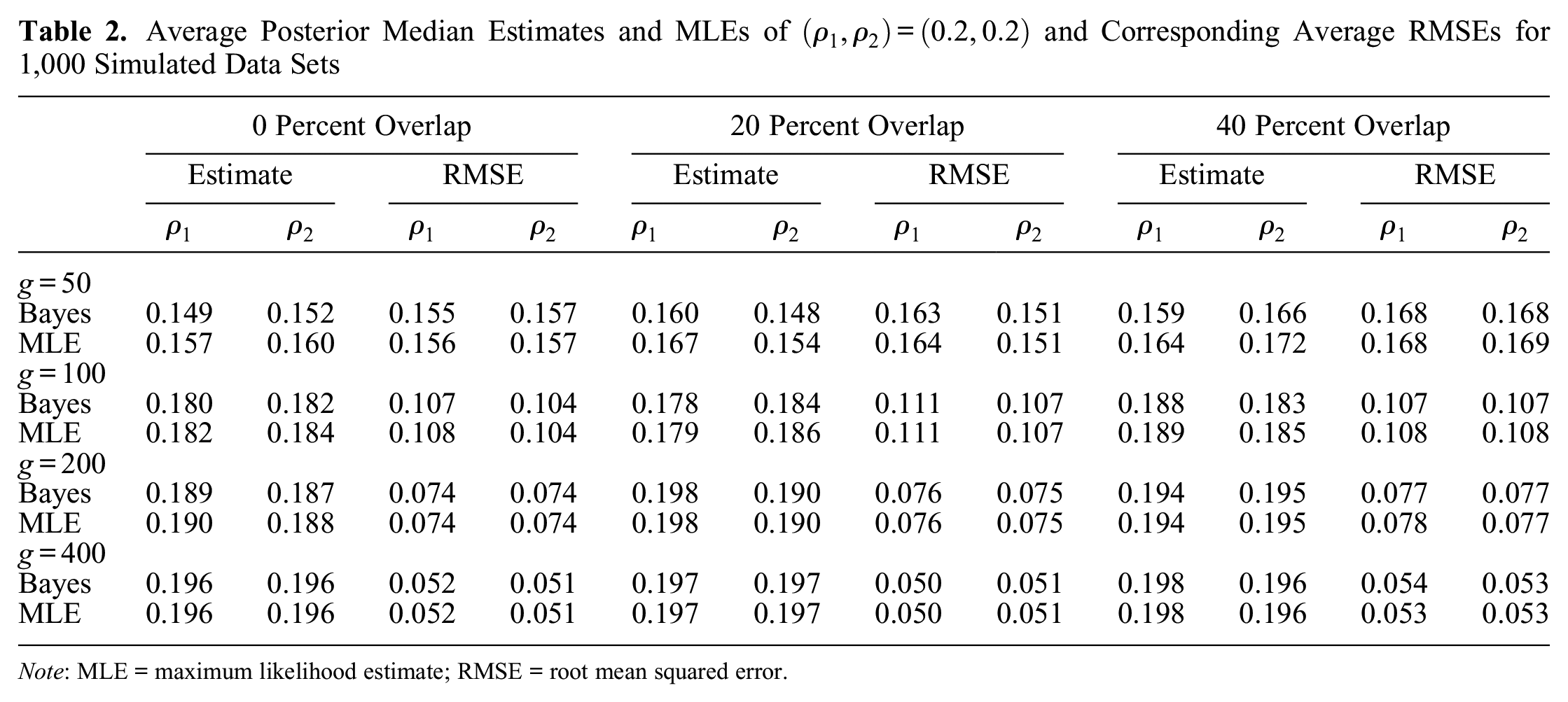
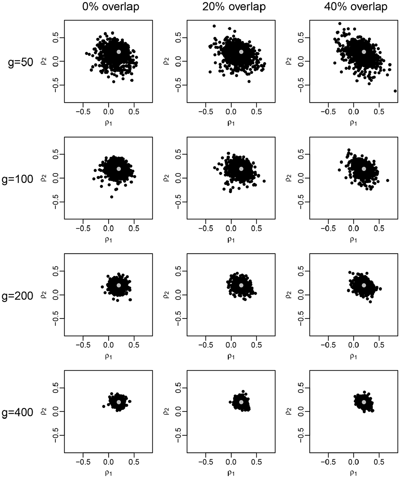
Table 2 shows the average estimates and root mean squared errors of ${\rho }_1$ and ${\rho }_2$ for the Bayesian as well as the maximum likelihood estimator. Overall, the two estimators yield nearly identical results for all considered scenarios. As expected, the (negative) bias in the estimation of the network effects and the associated root mean squared errors are decreasing with the network size, the bias being virtually nonexistent for $g=400$ . Introducing 20 percent and 40 percent overlap between two connectivity matrices does not appear to affect the estimation results, even if there is mild negative correlation between the estimated network effects in these cases (see Figure 5).

Table 2.

Average Posterior Median Estimates and MLEs of $({\rho }_1,{\rho }_2)=(0.2,0.2)$ and Corresponding Average RMSEs for 1,000 Simulated Data Sets

	0 Percent Overlap				20 Percent Overlap				40 Percent Overlap
	Estimate		RMSE		Estimate		RMSE		Estimate		RMSE
	${\rho }_1$	${\rho }_2$	${\rho }_1$	${\rho }_2$	${\rho }_1$	${\rho }_2$	${\rho }_1$	${\rho }_2$	${\rho }_1$	${\rho }_2$	${\rho }_1$	${\rho }_2$
$g=50$
Bayes	0.149	0.152	0.155	0.157	0.160	0.148	0.163	0.151	0.159	0.166	0.168	0.168
MLE	0.157	0.160	0.156	0.157	0.167	0.154	0.164	0.151	0.164	0.172	0.168	0.169
$g=100$
Bayes	0.180	0.182	0.107	0.104	0.178	0.184	0.111	0.107	0.188	0.183	0.107	0.107
MLE	0.182	0.184	0.108	0.104	0.179	0.186	0.111	0.107	0.189	0.185	0.108	0.108
$g=200$
Bayes	0.189	0.187	0.074	0.074	0.198	0.190	0.076	0.075	0.194	0.195	0.077	0.077
MLE	0.190	0.188	0.074	0.074	0.198	0.190	0.076	0.075	0.194	0.195	0.078	0.077
$g=400$
Bayes	0.196	0.196	0.052	0.051	0.197	0.197	0.050	0.051	0.198	0.196	0.054	0.053
MLE	0.196	0.196	0.052	0.051	0.197	0.197	0.050	0.051	0.198	0.196	0.053	0.053

Note: MLE = maximum likelihood estimate; RMSE = root mean squared error.

Figure 5.

Posterior median estimates (black) of $({\rho }_1,{\rho }_2)=(0.2,0.2)$ (gray) for 1,000 simulated data sets.

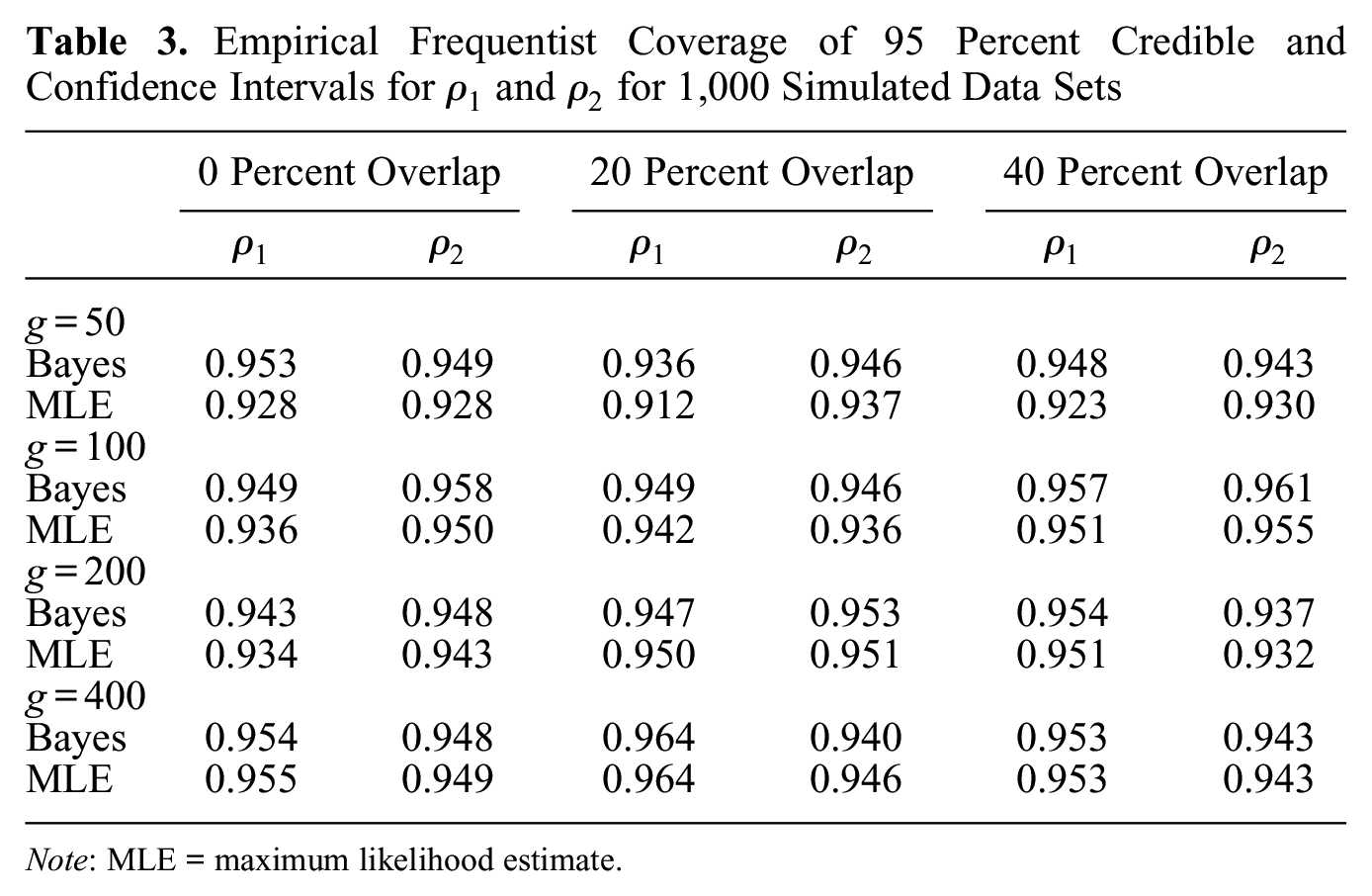
Table 3 reports the empirical frequentist coverage of Bayesian equal-tailed 95 percent credible intervals and asymptotic 95 percent maximum likelihood-based confidence intervals for ${\rho }_1$ and ${\rho }_2$ . The coverage of Bayesian credible intervals is very close to the nominal 0.95 for all considered scenarios, and the coverage of confidence intervals is below nominal for network sizes of 50. These observations are in line with the subpar coverage of maximum likelihood-based confidence intervals for small samples in the first-order network autocorrelation model reported by Dittrich et al. (2017a).

Table 3.

Empirical Frequentist Coverage of 95 Percent Credible and Confidence Intervals for ${\rho }_1$ and ${\rho }_2$ for 1,000 Simulated Data Sets

	0 Percent Overlap		20 Percent Overlap		40 Percent Overlap
	${\rho }_1$	${\rho }_2$	${\rho }_1$	${\rho }_2$	${\rho }_1$	${\rho }_2$
$g=50$
Bayes	0.953	0.949	0.936	0.946	0.948	0.943
MLE	0.928	0.928	0.912	0.937	0.923	0.930
$g=100$
Bayes	0.949	0.958	0.949	0.946	0.957	0.961
MLE	0.936	0.950	0.942	0.936	0.951	0.955
$g=200$
Bayes	0.943	0.948	0.947	0.953	0.954	0.937
MLE	0.934	0.943	0.950	0.951	0.951	0.932
$g=400$
Bayes	0.954	0.948	0.964	0.940	0.953	0.943
MLE	0.955	0.949	0.964	0.946	0.953	0.943

Note: MLE = maximum likelihood estimate.

On the basis of results from our first simulation experiment, we draw two main conclusions. First, we recommend using the Bayesian estimator over the maximum likelihood estimator, as both estimators yield nearly identical network effect estimates, but the coverage of Bayesian credible intervals appears accurate, whereas for smaller network sizes the coverage of maximum likelihood-based confidence intervals is much less accurate. Second, estimating second-order network autocorrelation models with moderately overlapping connectivity matrices, that is, with up to 40 percent shared ties, does not affect estimation of the network effects. This second finding is of particular importance to social network researchers who often encounter distinct but partially overlapping networks in empirical practice.

Figure 6 displays the average logarithm of the Bayes factor of hypothesis $H_1$ (thick solid line), $H_2$ (thick dashed line), $H_3$ (dotted line), $H_4$ (dashed line), and $H_5$ (solid line) against an unconstrained reference hypothesis, $H_u$ , respectively, as a function of network effects $({\rho }_1,{\rho }_2)$ from $(0.40,0)$ to $(0,0.40)$ . Overall, the results indicate that the Bayes factor shows consistent behavior, that is, there is the most evidence for the data-generating hypothesis if the network size is large enough. This evidence monotonically increases with network size. In particular, there is little discrimination between the five hypotheses for $g=50$ , whereas there is clear support for the data-generating hypothesis for network sizes of 200 and 400. Two lines in Figure 6 are discontinued for numerical reasons: when computing the Bayes factor, we need to calculate the probability mass of the unconstrained importance density contained in the parameter space imposed by the constraints under a hypothesis (see Appendix B). For the Bayes factors involving the purely inequality constrained hypotheses $H_2:{\rho }_1>{\rho }_2>0$ and $H_4:0<{\rho }_1<{\rho }_2$ , we approximated these probabilities numerically by the proportion of 1,000 draws from the unconstrained importance densities that were in agreement with hypothesis $H_2$ and hypothesis $H_4$ , respectively. For some data sets, however, none of the draws were in agreement with hypothesis $H_2$ , or hypothesis $H_4$ , in which case we set the corresponding marginal likelihood to $-\infty$ . If this happened for at least one of the 100 simulated data sets, then the average logarithm of the Bayes factor was $-\infty$ as well. Finally, as in our first simulation experiment, these findings are robust to moderate degrees of overlap between two connectivity matrices.

Figure 6.

Average logarithm of the Bayes factors $\log \left(B_{\mathrm{tu}}\right)$ , $t\in \{1,2,3,4,5\}$ , of the hypotheses $H_1:{\rho }_1>{\rho }_2=0$ (thick solid line), $H_2:{\rho }_1>{\rho }_2>0$ (thick dashed line), $H_3:{\rho }_1={\rho }_2>0$ (dotted line), $H_4:0<{\rho }_1<{\rho }_2$ (dashed line), and $H_5:0={\rho }_1<{\rho }_2$ (solid line) against $H_u:({\rho }_1,{\rho }_2)\in {\Theta }_{({\rho }_1,{\rho }_2)}$ as a function of network effects $({\rho }_1,{\rho }_2)$ from $(0.40,0)$ to $(0,0.40)$ for 100 simulated data sets.

6. Application Revisited

In this section, we reanalyze a data set from the economic growth literature initially studied by Dall’erba et al. (2009) and address the questions raised in Section 2.3. First, we reestimated the second-order network autocorrelation model in equation (4) on the basis of noninformative priors for all model parameters and compared the results with those coming from maximum likelihood estimation. Second, we used Bayes factors to quantify the relative evidence in the data for different competing hypotheses of interest with respect to this data set. Finally, we considered a network autocorrelation model with two subgroups, assuming only one dominant common influence mechanism within and between the two subgroups.

6.1. Bayesian Estimation of a Second-Order Network Autocorrelation Model

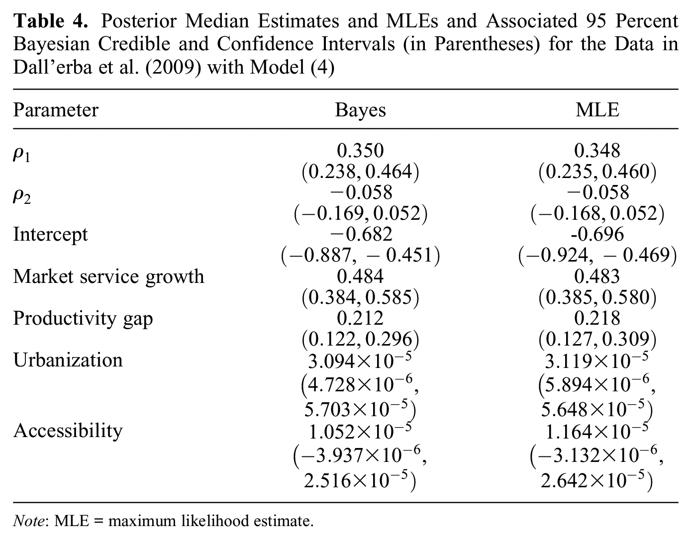
Table 4 displays the results of a Bayesian estimation of the second-order model in equation (4), along with the corresponding maximum likelihood estimates. ¹⁶ The Bayesian and the maximum likelihood estimates of all parameters are similar to each other, in line with results from our simulation study in Section 5.2. In particular, the (Bayesian) estimate of ${\rho }_1$ , reflecting interactions within the same country, is of large positive magnitude (0.350), and the (Bayesian) estimate of ${\rho }_2$ , reflecting spillovers from regions in neighboring countries, is much smaller and close to zero (–0.058). ¹⁷ Dall’erba et al. (2009) concluded by saying that “the results obtained also confirm the hypothesis that economic interactions decrease very substantially when a national border is passed (indeed, the coefficient reflecting external spillovers is not statistically significant)” (p. 342).

Table 4.

Posterior Median Estimates and MLEs and Associated 95 Percent Bayesian Credible and Confidence Intervals (in Parentheses) for the Data in Dall’erba et al. (2009) with Model (4)

Parameter	Bayes	MLE
${\rho }_1$	0.350 $(0.238,0.464)$	0.348 $(0.235,0.460)$
${\rho }_2$	−0.058 $(-0.169,0.052)$	−0.058 $(-0.168,0.052)$
Intercept	−0.682 $(-0.887,-0.451)$	-0.696 $(-0.924,-0.469)$
Market service growth	0.484 $(0.384,0.585)$	0.483 $(0.385,0.580)$
Productivity gap	0.212 $(0.122,0.296)$	0.218 $(0.127,0.309)$
Urbanization	$3.094\times {10}^{-5}$ $(4.728\times {10}^{-6},5.703\times {10}^{-5})$	$3.119\times {10}^{-5}$ $(5.894\times {10}^{-6},5.648\times {10}^{-5})$
Accessibility	$1.052\times {10}^{-5}$ $(-3.937\times {10}^{-6},2.516\times {10}^{-5})$	$1.164\times {10}^{-5}$ $(-3.132\times {10}^{-6},2.642\times {10}^{-5})$

Note: MLE = maximum likelihood estimate.

6.2. Bayesian Hypothesis Testing in a Second-Order Network Autocorrelation Model

Using Bayes factors, we quantified the evidence in the data for two hypotheses representing the notion of decreasing economic interactions once a national border is passed, $H_1:{\rho }_1>{\rho }_2=0$ and $H_2:{\rho }_1>{\rho }_2>0$ , and tested them against two competing hypotheses, $H_0:{\rho }_1={\rho }_2=0$ and $H_3:{\rho }_1={\rho }_2>0$ . ¹⁸ We also included a hypothesis $H_c:\neg (H_0\vee H_1\vee H_2\vee H_3)$ that represents the complement of all other possible hypotheses on $({\rho }_1,{\rho }_2)$ except hypotheses $H_0,H_1,H_2$ , and $H_3$ ; that is, hypothesis $H_c$ contains all the orders of network effects we did not hypothesize.

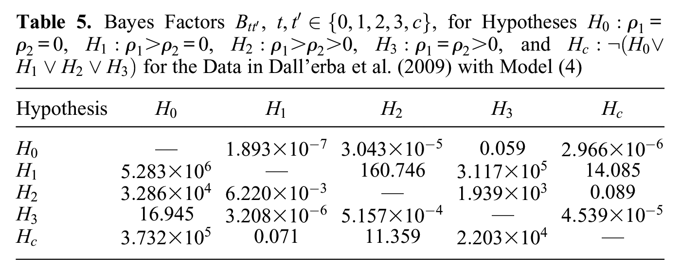
Table 5 provides the Bayes factors for every pair out of the set of the five considered hypotheses above using the prior specifications from Sections 4.2 and 4.3. Notably, $H_1:{\rho }_1>{\rho }_2=0$ is the hypothesis most supported by the data; it is approximately $5.3\times {10}^6$ , 160.7, $3.2\times {10}^5$ , and 14.1 times more supported than hypothesis $H_0$ , $H_2$ , $H_3$ , and $H_c$ , respectively. Moreover, we see the least evidence in the data in favor of the null. Consequently, regardless of the specification of alternative expectations about ${\rho }_1$ and ${\rho }_2$ , the hypothesis that both network effects are zero has to be strongly rejected. Although these implications seem in line with the authors’ claim that network effects decrease after a national border is passed, using Bayes factors provides us with much more extensive conclusions about the characteristic evidence in the data. Hence, we can now quantify how much more likely these conclusions are than competing conclusions (hypotheses) and how (un)likely it is that an entirely different mechanism $H_c$ generated the data. Ultimately, this data set contains the most and very strong evidence for a positive within-country network effect only.

Table 5.

Bayes Factors $B_{\mathrm{tt}\prime }$ , $t,t\prime \in \{0,1,2,3,c\}$ , for Hypotheses $H_0:{\rho }_1={\rho }_2=0$ , $H_1:{\rho }_1>{\rho }_2=0$ , $H_2:{\rho }_1>{\rho }_2>0$ , $H_3:{\rho }_1={\rho }_2>0$ , and $H_c:\neg (H_0\vee H_1\vee H_2\vee H_3)$ for the Data in Dall’erba et al. (2009) with Model (4)

Hypothesis	$H_0$	$H_1$	$H_2$	$H_3$	$H_c$
$H_0$	—	$1.893\times {10}^{-7}$	$3.043\times {10}^{-5}$	0.059	$2.966\times {10}^{-6}$
$H_1$	$5.283\times {10}^6$	—	160.746	$3.117\times {10}^5$	14.085
$H_2$	$3.286\times {10}^4$	$6.220\times {10}^{-3}$	—	$1.939\times {10}^3$	0.089
$H_3$	16.945	$3.208\times {10}^{-6}$	$5.157\times {10}^{-4}$	—	$4.539\times {10}^{-5}$
$H_c$	$3.732\times {10}^5$	0.071	11.359	$2.203\times {10}^4$	—

6.3. Bayesian Hypothesis Testing in a Fourth-Order Network Autocorrelation Model

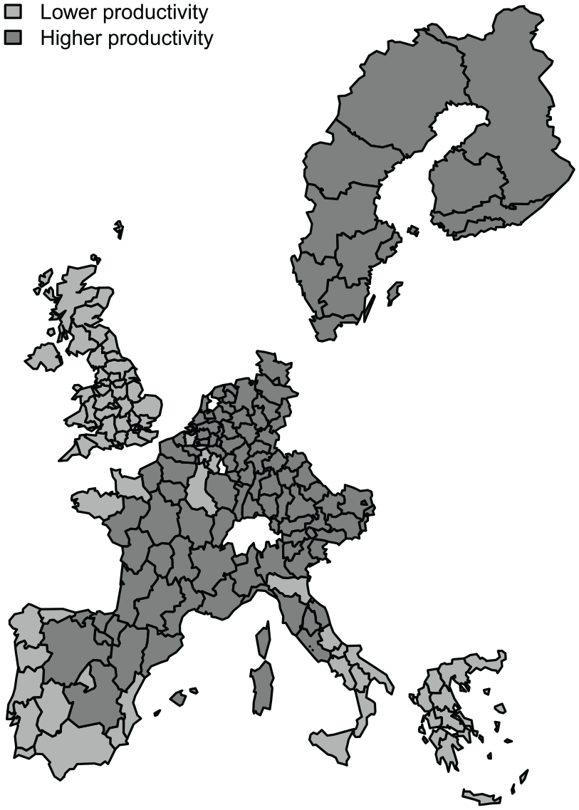
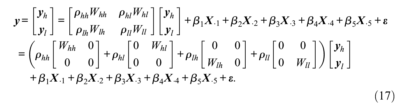
Dall’erba et al. (2009) pointed to potentially asymmetric growth rates across the regions, depending on a region’s initial productivity level. Thus, the authors proceeded by dividing the sample into two clusters: 111 initially more productive regions and 77 initially less productive regions, implying a core-periphery pattern (see Figure 7). ¹⁹ Next, they separately estimated two second-order network autocorrelation models for the two clusters. Here, for illustrative purposes, we allowed for varying levels of network autocorrelation within and between the two clusters and consider a model with two subgroups instead. For example, we could expect network effects within regions of the same subgroup to be larger than network effects between regions of different subgroups, or we could expect initially more productive regions to influence initially less productive ones more strongly than the other way around.

Figure 7.

Spatial distribution of productivity levels in 1980 across the 188 regions.

Our analyses in Section 6.2 suggest that there is very strong evidence in the data for a positive within-country network effect only; that is, ${\rho }_1>0$ and ${\rho }_2=0$ . Thus, we merely considered spillover effects within the same country, in other words, we assume only $W_1$ plays a role, not $W_2$ . We denote by ${\rho }_{\mathrm{hh}},{\rho }_{\mathrm{hl}},{\rho }_{\mathrm{lh}}$ , and ${\rho }_{\mathrm{ll}}$ the network effect within regions with initially higher productivity levels, the network effect of initially less productive regions on initially more productive regions, the network effect of initially more productive regions on initially less productive ones, and the network effect within regions with initially lower productivity levels, respectively. Accordingly, ${\mathit{y}}_h\in {\mathbb{R}}^{111}$ and ${\mathit{y}}_l\in {\mathbb{R}}^{77}$ contain the growth rates of labor productivity of the initially more and less productive regions, respectively, and we partitioned $W_1$ , the unstandardized connectivity matrix using the region’s three nearest neighbors within the same country, into the four submatrices $W_{\mathrm{hh}}\in {\mathbb{R}}^{111\times 111}$ , $W_{\mathrm{hl}}\in {\mathbb{R}}^{111\times 77}$ , $W_{\mathrm{lh}}\in {\mathbb{R}}^{77\times 111}$ , and $W_{\mathrm{ll}}\in {\mathbb{R}}^{77\times 77}$ , representing ties within and between the two subgroups. ²⁰ This results in the following fourth-order network autocorrelation model

$$\begin{array}{l}\mathrm{y}=\left[\begin{array}{c}{\mathrm{y}}_h\\ {\mathrm{y}}_l\end{array}\right]=\left[\begin{array}{cc}{\rho }_{hh}{W}_{hh}& {\rho }_{hl}{W}_{hl}\\ {\rho }_{lh}{W}_{lh}& {\rho }_{ll}{W}_{ll}\end{array}\right]\left[\begin{array}{c}{\mathrm{y}}_h\\ {\mathrm{y}}_l\end{array}\right]+{\beta }_1{\mathrm{X}}_{\cdot 1}+{\beta }_2{\mathrm{X}}_{\cdot 2}+{\beta }_3{\mathrm{X}}_{\cdot 3}+{\beta }_4{\mathrm{X}}_{\cdot 4}+{\beta }_5{\mathrm{X}}_{\cdot 5}+\epsilon \\ \begin{array}{l}=\left({\rho }_{hh}\left[\begin{array}{cc}{W}_{hh}& 0\\ 0& 0\end{array}\right]+{\rho }_{hl}\left[\begin{array}{cc}0& W_{hl}\\ 0& 0\end{array}\right]+{\rho }_{lh}\left[\begin{array}{cc}0& 0\\ W_{lh}& 0\end{array}\right]+{\rho }_{ll}\left[\begin{array}{cc}0& 0\\ 0& W_{ll}\end{array}\right]\right)\left[\begin{array}{c}{\mathrm{y}}_h\\ {\mathrm{y}}_l\end{array}\right]\hfill \\ +{\beta }_1{\mathrm{X}}_{\cdot 1}+{\beta }_2{\mathrm{X}}_{\cdot 2}+{\beta }_3{\mathrm{X}}_{\cdot 3}+{\beta }_4{\mathrm{X}}_{\cdot 4}+{\beta }_5{\mathrm{X}}_{\cdot 5}+\epsilon .\hfill \end{array}\end{array}$$

(17)

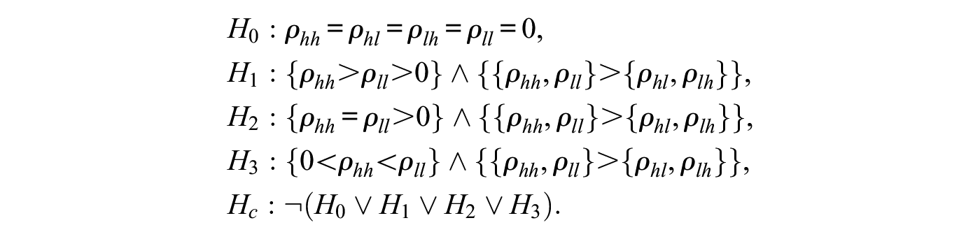
We generally expect the network effects within the two subgroups to be larger than the network effects between subgroups, that is, $\{{\rho }_{\mathrm{hh}},{\rho }_{\mathrm{ll}}\}>\{{\rho }_{\mathrm{hl}},{\rho }_{\mathrm{lh}}\}$ , where the “>” sign holds pairwise for any two elements of the first and second set, respectively. Furthermore, hypotheses of substantial interest might be based on expectations of positive network effects within both subgroups but with potentially differing magnitudes. We translated these expectations to three hypotheses, $H_1,H_2$ , and $H_3$ , and supplemented them with the hypothesis of no network effects and the complement of all the orders of network effects we did not have hypotheses for. ²¹ Formally,

$$\begin{array}{c}{H}_0:{\rho }_{\mathrm{hh}}={\rho }_{\mathrm{hl}}={\rho }_{\mathrm{lh}}={\rho }_{\mathrm{ll}}=0,\hfill \\ H_1:\{{\rho }_{\mathrm{hh}}>{\rho }_{\mathrm{ll}}>0\}\wedge \{\{{\rho }_{\mathrm{hh}},{\rho }_{\mathrm{ll}}\}>\{{\rho }_{\mathrm{hl}},{\rho }_{\mathrm{lh}}\}\},\hfill \\ H_2:\{{\rho }_{\mathrm{hh}}={\rho }_{\mathrm{ll}}>0\}\wedge \{\{{\rho }_{\mathrm{hh}},{\rho }_{\mathrm{ll}}\}>\{{\rho }_{\mathrm{hl}},{\rho }_{\mathrm{lh}}\}\},\hfill \\ H_3:\{0<{\rho }_{\mathrm{hh}}<{\rho }_{\mathrm{ll}}\}\wedge \{\{{\rho }_{\mathrm{hh}},{\rho }_{\mathrm{ll}}\}>\{{\rho }_{\mathrm{hl}},{\rho }_{\mathrm{lh}}\}\},\hfill \\ H_c:\neg (H_0\vee H_1\vee H_2\vee H_3).\hfill \end{array}$$

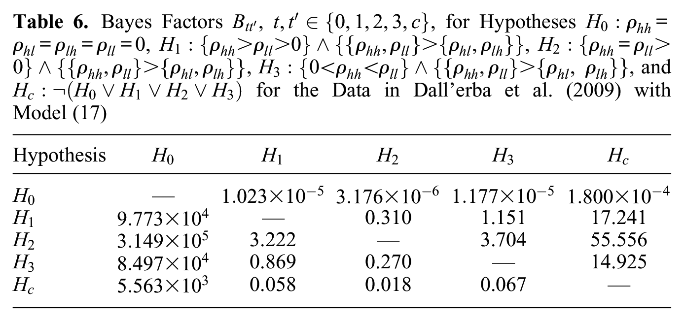
Table 6 shows the Bayes factors for every pair out of the set of the five considered hypotheses. We see that $H_2:\{{\rho }_{\mathrm{hh}}={\rho }_{\mathrm{ll}}>0\}\wedge \{\{{\rho }_{\mathrm{hh}},{\rho }_{\mathrm{ll}}\}>\{{\rho }_{\mathrm{hl}},{\rho }_{\mathrm{lh}}\}\}$ is the hypothesis most supported by the data; it receives approximately $3.1\times {10}^5$ , 3.2, 3.7, and 55.6 times more support than do hypothesis $H_0$ , $H_1$ , $H_3$ , and $H_c$ , respectively. Hence, there is no evidence in the data for differing network effects within the initially more and less productive regions, but there is very strong evidence that network effects within the two subgroups are larger than network effects between subgroups.

Table 6.

Bayes Factors $B_{\mathrm{tt}\prime }$ , $t,t\prime \in \{0,1,2,3,c\}$ , for Hypotheses $H_0:{\rho }_{\mathrm{hh}}={\rho }_{\mathrm{hl}}={\rho }_{\mathrm{lh}}={\rho }_{\mathrm{ll}}=0$ , $H_1:\{{\rho }_{\mathrm{hh}}>{\rho }_{\mathrm{ll}}>0\}\wedge \{\{{\rho }_{\mathrm{hh}},{\rho }_{\mathrm{ll}}\}>\{{\rho }_{\mathrm{hl}},{\rho }_{\mathrm{lh}}\}\}$ , $H_2:\{{\rho }_{\mathrm{hh}}={\rho }_{\mathrm{ll}}>0\}\wedge \{\{{\rho }_{\mathrm{hh}},{\rho }_{\mathrm{ll}}\}>\{{\rho }_{\mathrm{hl}},{\rho }_{\mathrm{lh}}\}\}$ , $H_3:\{0<{\rho }_{\mathrm{hh}}<{\rho }_{\mathrm{ll}}\}\wedge \{\{{\rho }_{\mathrm{hh}},{\rho }_{\mathrm{ll}}\}>\{{\rho }_{\mathrm{hl}},{\rho }_{\mathrm{lh}}\}\}$ , and $H_c:\neg (H_0\vee H_1\vee H_2\vee H_3)$ for the Data in Dall’erba et al. (2009) with Model (17)

Hypothesis	$H_0$	$H_1$	$H_2$	$H_3$	$H_c$
$H_0$	—	$1.023\times {10}^{-5}$	$3.176\times {10}^{-6}$	$1.177\times {10}^{-5}$	$1.800\times {10}^{-4}$
$H_1$	$9.773\times {10}^4$	—	0.310	1.151	17.241
$H_2$	$3.149\times {10}^5$	3.222	—	3.704	55.556
$H_3$	$8.497\times {10}^4$	0.869	0.270	—	14.925
$H_c$	$5.563\times {10}^3$	0.058	0.018	0.067	—

7. Conclusions

In this article, we developed Bayesian techniques for estimating and, primarily, testing higher-order network autocorrelation models with multiple network autocorrelations. In particular, we provided default Bayes factors that enable researchers to test hypotheses with order constraints on the network effects in a direct manner. The proposed methods allow researchers to simultaneously test any number of competing hypotheses on the relative strength of network effects against one another and to quantify the amount of evidence in the data for each hypothesis. This has not yet been possible using currently available statistical techniques for network autocorrelation models. Our proposed methods can straightforwardly be extended to test hypotheses on network autocorrelation parameters in heteroskedastic network autocorrelation models (LeSage 1997a) and network disturbances models (Leenders 2002).

We ran a simulation study to evaluate the numerical behavior of the presented Bayesian procedures for a number of different network specifications, including varying network sizes and network overlap. Our simulation study showed that, first, the Bayesian estimator and the maximum likelihood estimator yield similar parameter estimates of the network autocorrelation parameters for all scenarios. This was expected because we relied on noninformative priors for the network autocorrelation parameters. As a next step, it would be interesting to explore the use of (weakly) informative priors for multiple network autocorrelation parameters. Such priors can either be derived from published estimates in previous literature (similar to what Dittrich et al. [2017a] did for the first-order network autocorrelation model) or by eliciting experts on anticipated network effects in a given case study. Given previous findings in the literature when using a weakly informative prior for estimating a single network autocorrelation parameter (Dittrich et al. 2017a), we expect a carefully specified weakly informative prior for multiple network autocorrelation parameters will also decrease the negative bias of network autocorrelation parameters associated with maximum likelihood estimation of the model. Second, the Bayesian estimator exhibits nominal coverage of credible intervals and is more accurate than the maximum likelihood estimator, which is a strong argument in favor of the Bayesian approach, even when noninformative priors are used. Third, we found that the proposed Bayes factors always result in the largest evidence for the true data-generating hypothesis, with this evidence increasing further with network size. In other words, the proposed Bayes factors tend to point researchers to the correct (or best) hypothesis out of a set of competing hypotheses; these hypotheses can represent highly complex relations between the autocorrelation parameters, and the set of hypotheses tested against each other simultaneously can, in principle, be arbitrarily large.

The practical tools needed to perform the methods developed in this article are, or will be, freely accessible in an R package. Given the many, often implicit, expectations researchers have about the relative importance of different network effects, we hope that by enabling researchers to test these expectations directly and explicitly, higher-order network autocorrelation models will bring forth a more thorough understanding of social contagion processes that goes beyond the current state of the art.