Robustness and Model Selection in Configurational Causal Modeling

Abstract

In recent years, proponents of configurational comparative methods (CCMs) have advanced various dimensions of robustness as instrumental to model selection. But these robustness considerations have not led to computable robustness measures, and they have typically been applied to the analysis of real-life data with unknown underlying causal structures, rendering it impossible to determine exactly how they influence the correctness of selected models. This article develops a computable criterion of fit-robustness, which quantifies the degree to which a CCM model agrees with other models inferred from the same data under systematically varied threshold settings of fit parameters. Based on two extended series of inverse search trials on data simulated from known causal structures, the article moreover provides a precise assessment of the degree to which fit-robustness scoring is conducive to finding a correct causal model and how it compares to other approaches of model selection.

Keywords

causal modeling configurational comparative methods Coincidence Analysis Qualitative Comparative Analysis model selection robustness

Introduction

Different methods of causal data analysis tend to track different features of causal structures, exploit different markers in empirical data for their inference to causation, or define causation along the lines of different theories of causation. These differences must be taken into account when benchmarking the issued models. This holds notably for model robustness. What it means for a model to be robust depends on what the corresponding method’s aims and purposes are. More concretely, the models of a method aiming, say, to quantify effect sizes on the population level must meet different robustness criteria than the models of a method aiming to capture difference-making relations on the case level. It follows that different criteria are needed for different methods. While some methodological frameworks have long traditions of robustness benchmarking, others do not. A framework of the latter type is the one of configurational comparative methods (CCMs; see, e.g., Baumgartner and Ambühl 2020; Cronqvist and Berg-Schlosser 2009; Ragin 2008; Thiem 2014b), where discussions about robustness have begun only recently. The goal of this article is to contribute to the ongoing development of robustness benchmarks custom-built for the aims and purposes of CCMs.

The most widely employed robustness measures are the ones of causal discovery methods using statistical techniques. Such methods, as regression analysis (e.g., Gelman and Hill 2007) or Bayes-nets methods (e.g., Spirtes, Glymour, and Scheines 2000), rely on probabilistic or counterfactual theories of causation (e.g., Lewis 1973; Suppes 1970), they track causal dependencies between random variables (e.g. “X is a cause of Y”), and, most importantly, their models are built to reflect average or marginal effect sizes or net effects in the whole data. Their models count as robust only if they remain invariant across repeated re-analyses of the data under subsampling, measurement error introduction, or variation of tuning parameters. CCMs, by contrast, rely on regularity theories of causation (e.g., Mackie 1974), they track causal dependencies between specific values of variables (e.g., “X= $χ$ is a cause of Y= $γ$ ”), they analyze conjunctural causation and equifinality (i.e., not marginal effect sizes) and—following the template of Mill’s method of difference—their models are intended to reflect difference-making relations on the level of individual cases in the data. More concretely, if the data contain cases that vary in exactly one of the analyzed factors as well as in the outcome, while all other factors remain constant, CCMs take this as evidence for the causal relevance of a value of the varying factor.¹ Therefore, adding, subtracting, or recoding a few cases, say, due to varying tuning parameters or measurement error introduction, frequently amounts to altering difference-making evidence, which then induces changes in CCM models. As CCM models are expressly built to reflect cross-case variation, robustness measures that reward model invariance miss the very aim of CCMs.

Nonetheless, some authors have recently benchmarked CCM models against statistical robustness standards (e.g., Hug 2013; Krogslund, Choi, and Poertner 2015). The results are seemingly devastating for CCMs, as their models typically do not meet these standards to an acceptable degree. But that finding, rather than yielding a meaningful estimate of the robustness of CCM models and demonstrating their unreliability, as Hug (2013) and Krogslund et al. (2015) submit, merely exhibits that a robustness measure rewarding invariance is at cross purposes with CCMs.

A lot of variance in CCM models is completely benign. It simply reflects varying amounts of inferentially exploited difference-making evidence without implying any inconsistent causal conclusions. Two different models are in no disagreement if the causal claims entailed by them stand in a subset relation, that is, if one of them is a submodel of the other. In that case, the submodel merely recovers the data-generating structure less completely than the supermodel. But given the massive fragmentation of data commonly analyzed by CCMs, CCMs cannot normally be expected to uncover data-generating structures in their entirety anyway. Importantly, CCM models only make claims about causal relevance, not about causal irrelevance. If a factor value X= $χ$ does not appear in a model of an outcome Y= $γ$ , it does not follow that X= $χ$ is causally irrelevant to Y= $γ$ but only that the data do not contain evidence for the relevance of X= $χ$ (Baumgartner and Ambühl 2020).

However, not all variance in CCM models is of the benign kind. For example, it regularly happens that data entail many different models that are not submodels of one another, giving rise to model ambiguities (Baumgartner and Thiem 2017). Criteria are needed that select among such unrelated models. Or, maximizing the two core parameters of model fit, namely, consistency and coverage, tends to induce CCMs to expand resulting models by irrelevant factor values, prompting overfitting and corresponding false positives (see the section Overfitting; Arel-Bundock 2019). Strategies are needed to avoid that pitfall. Hence, there is a need for distinguishing benign from non-benign model variance and, more generally, for complementing existing criteria of model selection by additional constraints. Robustness standards—properly adapted to the purposes of CCMs—are straightforward candidates to fill that bill.

Indeed, in recent years, proponents of CCMs have advanced various dimensions of robustness as instrumental to model selection (e.g., Cooper and Glaesser 2016; Schneider and Wagemann 2012: $§$ 11.2; Skaaning 2011). But these discussions have typically revolved around concrete real-life data sets with unknown underlying causal structures.² In consequence, it is not possible to determine to what degree existing CCM robustness considerations are conducive to selecting correct models, avoiding overfitting, or reducing model ambiguities. Moreover, while there are numerous concrete illustrations qualitatively comparing different model candidates with respect to their robustness, there currently exist no computable robustness measures for CCMs.³

This article develops a computable criterion of fit-robustness that is tailor-made for CCMs by measuring the degree to which a model’s causal ascriptions overlap with the causal ascriptions of other models inferred from the same data under systematically varied fit thresholds. More specifically, our operationalization of robustness involves two steps: First, the set of all models $M$ for given data $δ$ is built by re-analyzing $δ$ under systematically varied consistency and coverage thresholds; second, the robustness of a particular model $m_{i} \in M$ is expressed in terms of the total number of sub- and supermodels $m_{i}$ has among the elements of $M$ . The more sub- and supermodels $m_{i}$ has in $M$ , the more $m_{i}$ overlaps in causal ascriptions with other models inferred from $δ$ , the higher $m_{i}$ ’s robustness score. By systematically varying other tuning parameters in the first step, analogous criteria of, say, calibration-robustness or frequency-robustness could be developed. For reasons of space, we focus on varying consistency and coverage only—which, after all, are the two dominant CCM criteria of model selection. Furthermore, for reasons of generality and computational flexibility, we will use Coincidence Analysis (CNA) as our CCM of choice. While Qualitative Comparative Analysis (QCA)—the best known CCM—only imposes consistency thresholds and comes with a search protocol for structures with single outcomes only, CNA accepts both consistency and coverage thresholds and can also analyze multi-outcome structures.

This article is organized as follows. The second section reviews the conceptual preliminaries of our argument. In the third section, we demonstrate the need for complementing existing criteria of model selection by a robustness criterion, whose details are presented in the fourth section. The fifth section benchmarks that criterion under a range of discovery conditions. We conclude in the sixth section. The Online Supplementary Material provides detailed R-scripts that supply an explicit R function operationalizing our robustness scoring and allow for replicating our benchmark tests along with all other calculations of this article.

Preliminaries

We begin by introducing the notation and the relevant concepts used in our ensuing discussion. CCMs study Boolean dependence relations between variables taking on specific values. In the CCM literature, variables are typically referred to as factors. Factors represent categorical properties that partition sets of units of observation (cases) either into two sets, in case of binary properties, or into more than two (but finitely many) sets, in case of multi-value properties. Factors representing binary properties can be crisp-set ( $c s$ ) or fuzzy-set ( $f s$ ); the former (typically) take on 0 and 1 as possible values, whereas the latter can take on any (continuous) values from the unit interval $[0, 1]$ . Factors representing multi-value properties are called multi-value ( $m v$ ) factors; they can take on any of an open (but finite) number of non-negative integers as possible values.

For simplicity of exposition, we will subsequently illustrate our robustness account with examples featuring binary factors only. This allows us to conveniently abbreviate the explicit “Factor $=$ value” notation. As is conventional in Boolean algebra, we write “A” for A=1 and “a” for A=0. While this shorthand simplifies the syntax of models, it introduces a risk of misinterpretation, for it yields that the factor A and its taking on the value 1 are both expressed by “A.” Disambiguation must hence be facilitated by the concrete context in which “A” appears. Accordingly, whenever we do not explicitly characterize italicized Roman letters as “factors,” we use them in terms of the shorthand notation. Moreover, we write “ $A * B$ ” for the conjunction “A=1 and B=1,” “ $A + B$ ” for the disjunction “A=1 or B=1,” “ $A \to B$ ” for the implication “If A=1, then B=1” ( $a + B$ ), and “ $A \leftrightarrow B$ ” for the equivalence “A=1 if, and only if, B=1” ( $A * B + a * b$ ).

Based on the implication operator, the notions of sufficiency and necessity are defined, which are the two Boolean dependence relations exploited by CCMs: X is sufficient for Y if, and only if (iff), $X \to Y$ (“if X is given, then Y is given”), and X is necessary for Y iff $Y \to X$ (“if Y is given, then X is given”). As Boolean dependencies amount to mere patterns of co-occurrence, they carry no causal connotations whatsoever and, hence, mostly do not reflect causal relations. Still, some of them do. So-called regularity theories of causation are designed to filter out those sufficiency and necessity relations that do track causation. They accomplish this by imposing a rigorous non-redundancy constraint (Baumgartner and Falk 2019; Graßhoff and May 2001; Mackie 1974). Only minimally sufficient conditions contained in minimally necessary conditions track causation, where sufficient and necessary conditions are said to be minimal iff they do not comprise sufficient and necessary proper parts.

CNA models can be atomic or complex, representing single-outcome and multi-outcome structures, respectively. An atomic model has the form $Φ \leftrightarrow Y$ , where Y is an endogenous factor value (Y= $γ$ ) and $Φ$ stands for a minimally necessary disjunction of minimally sufficient conditions in disjunctive normal form (DNF),⁴ such that all factors in that DNF are different (and logically and conceptually independent) from one another and from Y. An atomic CNA model explains an endogenous factor value Y in terms of a redundancy-free DNF of exogenous factor values. A complex CNA model is a redundancy-free conjunction of atomic models of the form $(Φ_{1} \leftrightarrow Y_{1}) * \dots * (Φ_{n} \leftrightarrow Y_{n})$ .

Since configurational data $δ$ tend to feature various deficiencies, such as measurement error or confounding, expressions of type $Φ \leftrightarrow Y$ that strictly adhere to the equivalence operation (“ $\leftrightarrow$ “) often cannot be inferred from $δ$ . To relax the equivalence standards, Ragin (2006) introduced the fit parameters of consistency and coverage into the QCA protocol, which have subsequently also been imported into CNA (Baumgartner and Ambühl 2020). Informally put, consistency reflects the degree to which the behavior of an outcome obeys a corresponding sufficiency or necessity relationship or a whole model, whereas coverage reflects the degree to which a sufficiency or necessity relationship or a whole model accounts for the behavior of the corresponding outcome. The parameters take values from the unit interval, with 1 representing perfect consistency and coverage. What counts as acceptable scores on these parameters is defined in threshold values determined by the analyst prior to the application of CNA. The models meeting the chosen thresholds are output by CNA along with their specific consistency and coverage scores. The product of a model’s consistency and coverage scores, that is, its con-cov product, is interpreted as a measure for its overall model fit.

To clarify the causal interpretation of CNA models, consider the following complex exemplar:

(A * b + a * B \leftrightarrow C) * (C * f + D \leftrightarrow E) .

Functionally put, (1) claims that the presence of A in conjunction with the absence of B (i.e., b) as well as a in conjunction with B are two alternative minimally sufficient conditions of C (relative to the chosen consistency threshold) and that $C * f$ and D are two alternative minimally sufficient conditions of E. Moreover, both $A * b + a * B$ and $C * f + D$ are claimed to be minimally necessary for C and E (relative to the chosen coverage threshold). Against the background of a regularity theory, these functional relations can be causally interpreted as follows: (i) The factor values listed on the left-hand sides of “ $\leftrightarrow$ ” are directly causally relevant for the factor values on the right-hand sides; (ii) A and b are located on the same causal path to C, which differs from the path on which a and B are located, and C and f are located on the same path to E, which differs from D’s path; and (iii) $A * b$ and $a * B$ are two alternative indirect causes of E whose influence is mediated on a causal chain via C.

Importantly, CNA models are to be interpreted relative to the data $δ$ from which they have been inferred and to the threshold settings chosen for that inference. That is, (1) does not purport to be a complete representation of the causal structure behind $δ$ . (1) only details those causally relevant factor values along with those conjunctive, disjunctive, and sequential groupings for which $δ$ contain evidence at the chosen threshold settings. In particular, (1) does not exclude that some further factor value G might not also be causally relevant for C or E; (1) only entails claims about causal relevance, not about causal irrelevance. By extension, another CNA model, such as (2), inferred from $δ$ relative to, say, lower consistency and/or coverage thresholds does not conflict with model (1).

(A + B \leftrightarrow C) * (C + D \leftrightarrow E) .

(2) identifies A and B as alternative direct causes of C and indirect causes of E, moreover C and D are claimed to be alternative direct causes of E. All of this also follows from (1). The causal claims entailed by (2) thus constitute a subset of the claims entailed by (1), meaning that (2) is a submodel of (1). As the submodel relation will be of core relevance for our ensuing argument, we define it in all explicitness here.

Submodel Relation

A CCM model $m_{i}$ is a submodel of another CCM model $m_{j}$ if, and only if,

all factor values causally relevant according to $m_{i}$ are also causally relevant according to $m_{j}$ ,

all factor values contained in two different disjuncts in $m_{i}$ are also contained in two different disjuncts in $m_{j}$ ,

all factor values contained in the same conjunct in $m_{i}$ are also contained in the same conjunct in $m_{j}$ ,

if $m_{i}$ and $m_{j}$ are complex models, all atomic components $m_{i}^{k}$ of $m_{i}$ have a counterpart $m_{j}^{k}$ in $m_{j}$ , such that (1)–(3) are satisfied for $m_{i}^{k}$ and $m_{j}^{k}$ .

If $m_{i}$ is a submodel of $m_{j}$ , $m_{j}$ is a supermodel of $m_{i}$ . All of m _i’s causal ascriptions are contained in its supermodels’ ascriptions, and m _i contains the causal ascriptions of its own submodels. The submodel relation is reflexive: Every model is a submodel (and supermodel) of itself; or differently, if $m_{i}$ and $m_{j}$ are submodels of one another, then $m_{i}$ and $m_{j}$ are identical. Most importantly, even if two models related by the submodel relation are not identical, they do not disagree or conflict in their causal ascriptions; rather, they can be interpreted as describing the same causal structure with varying granularity.

Overfitting

Numerous authors (e.g., Braumoeller 2015; Krogslund et al. 2015; Lucas and Szatrowski 2014) have argued that CCMs have a dangerous tendency to incorporate causally irrelevant factors in their models, thereby committing too many false positive errors. Representatives of CCMs (e.g., Baumgartner and Thiem 2020; Rohlfing 2015; Thiem and Baumgartner 2016) have found various flaws and overgeneralizations in these arguments and have shown that CCMs work reliably for data conforming to the high-quality standards imposed by CCMs, in particular, the homogeneity of the unmeasured causal background.⁵ Still, the fact remains that CCMs run a serious false positive risk when these quality standards are not met (Arel-Bundock 2019; Baumgartner and Ambühl 2020), in particular, when the data comprise cases incompatible with the data-generating causal structure over the set of measured factors, meaning cases that, subject to that structure, should not exist. Such case incompatibilities can have different sources, for instance, measurement error or confounding. For brevity, we will subsequently often simply say that case incompatibilities are due to noise.

Of course, noise has a negative effect on the output quality of any method, but for CCMs, this effect is especially high when the data have small sample size and the analyst is maximizing the model fit, that is, consistency and coverage. To illustrate this problem, consider the data in Table 1A, which have been simulated from the very simple causal structure in (3) and one added irrelevant factor D.

A + B * C \leftrightarrow E .

More specifically, Table 1A is the result of, first, collecting one case instantiating each of the 16 configurations of the factors A, B, C, D, and E compatible with (3) and, second, replacing one case in these clean and complete data by a case that is incompatible with (3). The incompatible case, $c_{16}$ , is highlighted with gray shading. The only difference between the original case and $c_{16}$ is that the latter features E=0 where the former had E=1, meaning that this case incompatibility can be thought of as resulting from noise on the outcome E.

Table 1.

Effect of Random Error.

A)
Case	A	B	C	D	E
c ₁	0	0	0	1	0
c ₂	0	0	1	1	0
c ₃	1	1	1	1	1
c ₄	1	1	1	0	1
c ₅	1	1	0	1	1
c ₆	0	1	0	1	0
c ₇	0	0	1	0	0
c ₈	1	0	0	1	1
c ₉	0	1	1	0	1
$c_{10}$	0	1	1	1	1
$c_{11}$	1	1	0	0	1
$c_{12}$	0	0	0	0	0
$c_{13}$	1	0	0	0	1
$c_{14}$	0	1	0	0	0
$c_{15}$	1	0	1	1	1
$c_{16}$	1	0	1	0	0
B)
#	Models	Con	Cov	Thresholds	Correct
1	$A * c + A * D + B * C \leftrightarrow E$	1.00	1.00	$〈 1.00, 1.00 〉$	✗
2	$A * c + B * C \leftrightarrow E$	1.00	0.89	$〈 1.00, 0.85 〉$	✗
3	$A * B + A * D + B * C \leftrightarrow E$	1.00	0.89	$〈 1.00, 0.85 〉$	✗
4	$A * D + B * C \leftrightarrow E$	1.00	0.78	$〈 1.00, 0.75 〉$	✗
5	$A * B + A * c + A * D \leftrightarrow E$	1.00	0.78	$〈 1.00, 0.75 〉$	✗
6	$A + B * C \leftrightarrow E$	0.90	1.00	$〈 0.85, 1.00 〉$	✓
7	$A + B \leftrightarrow E$	0.75	1.00	$〈 0.75, 1.00 〉$	✓
8	$A + C * D \leftrightarrow E$	0.80	0.89	$〈 0.75, 0.85 〉$	✗
9	$A \leftrightarrow E$	0.88	0.78	$〈 0.75, 0.75 〉$	✓

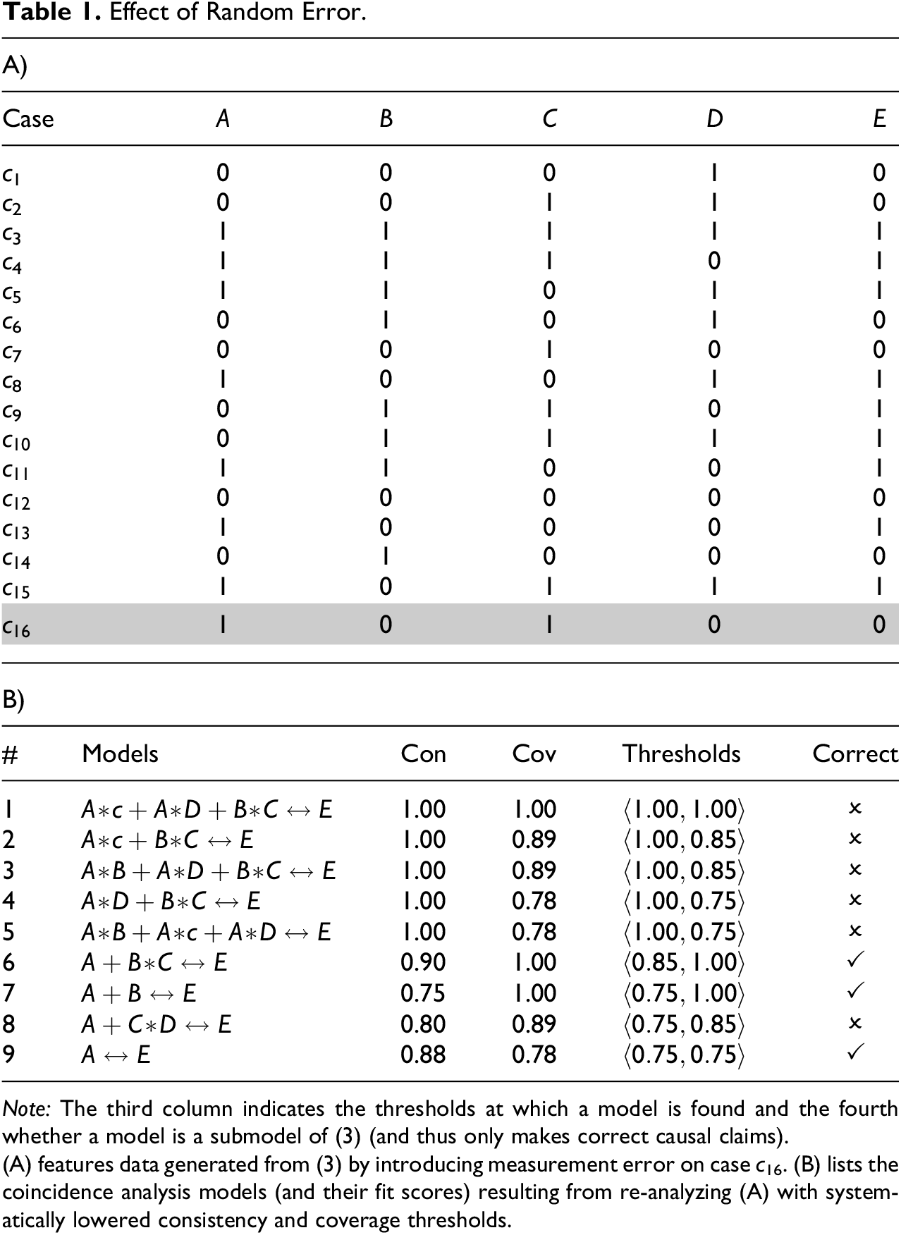
Note: The third column indicates the thresholds at which a model is found and the fourth whether a model is a submodel of (3) (and thus only makes correct causal claims).

(A) features data generated from (3) by introducing measurement error on case c ₁₆. (B) lists the coincidence analysis models (and their fit scores) resulting from re-analyzing (A) with systematically lowered consistency and coverage thresholds.

Case $c_{16}$ is incompatible with (3) because it does not feature the outcome E even though one of its causes in (3), A, is given. In light of $c_{16}$ , therefore, A cannot be identified as sufficient cause of E, meaning that, when processing Table 1A at maximal consistency and coverage thresholds of $〈 1, 1 〉$ , CNA (or QCA) will not recover (3). Instead, CNA will attempt to conjunctively complement A by further factor values in order to reach perfect consistency. Indeed, there exist two further factor values in combination with which A is strictly sufficient for E in Table 1A: $A * c$ and $A * D$ . It turns out, moreover, that disjunctively combining these two conditions with $B * C$ to $A * c + A * D + B * C$ yields perfect coverage. Accordingly, when CNA (or QCA) is run at $〈 1, 1 〉$ , it outputs model 1 in Table 1B (see the replication script for details). But, of course, given that (3) represents the ground truth, model 1 falsely ascribes causal relevance to c and D, which in fact are irrelevant.

Although not recovered at $〈 1, 1 〉$ , the data-generating structure (3) is a proper submodel of the model with maximal fit. And indeed, if the fit thresholds are lowered, CNA infers a whole array of further models from Table 1A, some of which are simpler than the best fitting model. Table 1B lists all models recovered when fit thresholds are systematically lowered from 1 to 0.75 at increments of 0.05. Some of these models yield false positives, but some exclusively entail causal claims that are correct according to the ground truth (3), namely, models 6, 7, and 9. Model 6, which is returned at a threshold setting of $〈 0.85, 1 〉$ , is identical to (3), while models 7 and 9 are proper submodels of (3).⁶ This shows that the false positives entailed by the model with maximal fit result from overfitting. When requested to maximize fit, CNA builds a disjunction comprising both irrelevant factor values and an irrelevant path. When the fit thresholds are relaxed, adding these additional factor values and the irrelevant path is no longer required to meet the thresholds, the overfitting disappears, and correct models are returned.

That CCMs fall prey to overfitting in the presence of only one single incompatible case is not some rare idiosyncrasy of Table 1A; rather, it is a commonplace phenomenon in small sample sizes.⁷ For CNA, the prevalence of overfitting can be demonstrated using the function cnaOpt() from the cnaOpt R-package (Ambühl and Baumgartner 2020), which purposefully builds models with maximal fit for the processed data. In what follows, we hence conduct a series of trials to determine the ratios of trials in which overfitting occurs by applying cnaOpt() to data sets with increasing sample sizes and increasing shares of incompatible cases. We again choose (3) as our ground truth and generate data from this structure relative to the factors A, B, C, D, and E; 16 configurations of these factors are compatible with (3). Let $δ^{i d}$ be the ideal data consisting of 16 cases, each of which instantiates another one of these 16 compatible configurations. In a first series of trials, we alternatively replace 1, 2, and 3 randomly drawn cases in $δ^{i d}$ by randomly drawn cases that are incompatible with (3), which yields increasing incompatibility shares (or noise ratios) of 6.25 percent, 12.5 percent, and 18.75 percent, respectively. In a second series, we double the case frequency resulting in 32 cases and again randomly replace 6.25 percent, 12.5 percent, and 18.75 percent compatible by incompatible cases. We repeat the same procedure for data sets of 48, 64, and 80 cases, thus multiplying the case frequency of $δ^{i d}$ by 3, 4, and 5. In each trial, we check whether the models generated by cnaOpt() are overfitted. The overfitting ratio for each trial is calculated based on 1,000 repetitions of the trial.

The results are plotted in Figure 1. It can easily be seen that they are damning for small sample sizes. At the base frequency of one case per compatible configuration, a single incompatible case leads to false positives due to overfitting in 38 percent of the trials. An incompatibility share of 12.5 percent, that is, two incompatible cases at $n = 16$ , pushes the overfitting ratio up to 67 percent, and at 18.75 percent incompatibilities, overfitting occurs in 80 percent of the trials. In larger sample sizes, the overfitting risk decreases. For instance, if the sample size and the number of case incompatibilities are multiplied by a factor of 4, the numbers come down to 0 percent, 1.4 percent, and 10.6 percent; and with even larger sample sizes, the overfitting risk becomes more and more negligible. Still, it is indisputable that the overfitting risk for small sample sizes is unacceptably high. After all, even in small samples—where it is common CCM practice not to select cases randomly but based on background theories and all available case knowledge (Schneider and Wagemann 2012)—the complete absence of incompatible cases can hardly ever be guaranteed in the disciplines in which CCMs are most often applied.

Figure 1.

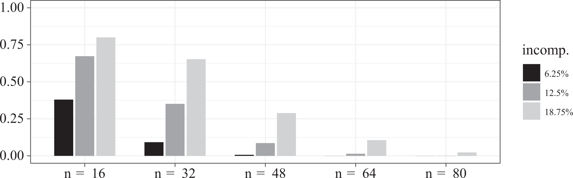
Overfitting ratios when processing data simulated from the target structure (3) with increasing sample sizes and increasing shares of randomly drawn incompatible cases. Each overfitting ratio is a mean over 1,000 executions of a trial.

The obvious conclusion to draw is that when analyzing small-sized noisy data, maximizing consistency and coverage is not a reliable strategy of model selection. This finding conflicts with certain methodological recommendations in the CCM literature. Ragin (2008:46), for instance, suggests that “[i]n general, consistency scores should be as close to 1.0 (perfect consistency) as possible”; or Schneider and Wagemann (2012:128) recommend that consistency thresholds be placed the higher, the lower the number of cases under investigation. However, in actual CCM practice, fit thresholds are often simply set to non-maximal bounds given by conventions, typically some values between 0.85 and 0.75; and in the example of Table 1A, such a conventional threshold placement avoids the overfitting problem. At $〈 0.75, 0.75 〉$ , a model is returned, namely, $A \leftrightarrow E$ , that merely assigns causal relevance to A, which is true according to the data-generating structure (3).⁸ Clearly though, the conventional threshold placement avoids the overfitting problem at the price of not revealing as much of the structure behind Table 1A as could possibly be revealed, for at $〈 0.85, 1 〉$ , the entire ground truth is correctly recoverable from Table 1A. In other words, $A \leftrightarrow E$ is not informative enough; it is not over- but underfitted.

Overall, in noisy discovery contexts, CCM model fit (just as model fit in other frameworks) should neither be maximized, to avoid overfitting, nor minimized, to avoid underfitting. Hence, the question arises how to identify threshold settings yielding models that are as revealing as possible about the ground truth without inducing false positives. In simulations, where the data-generating structure is presupposed, that question is easily answerable by re-analyzing the data at varying threshold settings and identifying the setting at which the (known) ground truth is recovered. But, of course, real-life discovery contexts are characterized by the data-generating structure being unknown, which makes it impossible to determine which among all tested threshold settings actually recovers the truth. To alleviate that problem, the next section introduces a criterion of fit-robustness that helps to identify the models that can be trusted among all the models returned by CCMs within the range of acceptable threshold settings.

Robustness

Searching for robust models to avoid over- and underfitting is an approach that comes easily to mind. But, as we have seen in the introduction, we cannot simply draw on statistical robustness measures rewarding model invariance under varying re-analyses of the data. Instead, we propose to understand the robustness of a CCM model in terms of the degree to which its causal attributions are contained in and contain the causal attributions of all the other models obtained from a series of data re-analyses under varying consistency and coverage settings. Rather than rewarding invariance, robustness in that sense rewards those models that are most closely interrelated with the other models from that re-analysis series and it punishes models making idiosyncratic causal attributions.

Before we flesh out that sketch, let us clarify the aims and limitations of our proposal. Robustness testing is a heuristic for model selection in noisy discovery contexts. If there is enough noise, especially if it is patterned or biased, any method will misfire sooner or later. But CCMs, as we have seen in the previous section, are particularly vulnerable through even mild degrees of noise. The purpose of a robustness measure for CCMs must be to reduce that vulnerability, without being expected to erase it altogether or to work equally well in all noise scenarios; it is only one tool for vulnerability reduction among others. In that light, the aim of our proposal shall be to improve the overall model quality in the presence of randomly distributed noise. The robustness measure sketched above can be expected to achieve that purpose because if measurement error is not biased and there is no systematic confounding (and there is not so much noise that CCMs abstain from drawing inferences altogether), the signal stemming from actual causal dependencies will, on average, be stronger in the data than spurious associations due to noise. In consequence, elements of the ground truth will be included in many models obtained at varying threshold settings, whereas spurious factor values will only be included in models inferred at specific consistency and coverage thresholds. That may not hold in biased and patterned noise scenarios. Thus, the next section will put the performance of our approach to the test under both random and non-random noise.

We now render our robustness measure precise on the basis of the submodel relation introduced in the section Preliminaries, which directly mirrors containment relations among causal attributions of CCM models. If two models are related in terms of the submodel relation, at most one of them makes causal attributions not made by the other one, such that the model with fewer attributions remains silent about the other model’s additional attributions. By contrast, if two models are not related by the submodel relation, they both entail some causal attributions not entailed by the other model. That is, the more sub- and supermodels a model $m_{i}$ has in a given set of models, the more $m_{i}$ ’s causal attributions overlap with the causal attributions of the other models in that set; conversely, the fewer the sub- and supermodels of $m_{i}$ , the more idiosyncratic $m_{i}$ ’s causal attributions. We thus propose to measure the fit-robustness of $m_{i}$ inferred from data $δ$ by re-analyzing $δ$ under systematically varied consistency and coverage settings and collecting all models returned in that re-analysis series in a set $M$ . The fit-robustness of $m_{i}$ can then be expressed in terms of the total number of sub- and supermodels $m_{i}$ has in $M$ .

This approach requires first producing a set $M$ of models inferable from $δ$ under systematically varied fit thresholds. The resulting robustness scoring is relative to the composition of $M$ , which, in turn, depends on two parameters: the scanned interval of threshold values and the granularity of the threshold variation. If we scan the interval $[0.8, 1]$ , $M$ typically only contains a proper subset of the models that result from scanning the interval $[0.7, 1]$ . Likewise, if we vary the consistency and coverage settings at increments of 0.1, less models tend to be recovered than if the settings are varied at a finer granularity of, say, 0.05. When combined, the scanned interval $[h, k]$ and the variation granularity l define a re-analysis type, which we simply denote by the tuple $〈 [h, k], l 〉$ . For example, the type $〈 [0.8, 1],0.1 〉$ scans the interval from consistency and coverage thresholds of 0.8 to 1 at increments of 0.1. When performed on a data set $δ$ , a re-analysis type yields a re-analysis series consisting of m analyses of $δ$ each of which is performed at a unique combination of consistency and coverage cutoffs. m is the number of two-element variations (with repetitions) of the sequence given by the interval and the granularity. More concretely, the type $〈 [0.8, 1],0.1 〉$ induces testing all two-element variations of the sequence ${0.8, 0.9, 1.0}$ , which amounts to $m = 9$ . Or differently, the re-analysis series performing that type tests the following consistency and coverage threshold pairs: $〈 0.8, 0.8 〉$ , $〈 0.9, 0.8 〉$ , $〈 1, 0.8 〉$ , $〈 0.8, 0.9 〉$ , $〈 0.9, 0.9 〉$ , $〈 1, 0.9 〉$ , $〈 0.8, 1 〉$ , $〈 0.9, 1 〉$ , and $〈 1, 1 〉$ .⁹ Collecting all models returned in the course of a re-analysis series results in a set of models $M$ for $δ$ relative to $〈 [h, k], l 〉$ . Taken together, these considerations yield the following notion of fit-robustness:

Fit-robustness (FR)

Given a set of models $M$ produced by a re-analysis series performing the re-analysis type $〈 [h, k], l 〉$ on data $δ$ , the fit-robustness of model $m_{i} \in M$ relative to $〈 [h, k], l 〉$ is the number of sub- and supermodels $m_{i}$ has in $M$ .

Before we illustrate (FR)-based robustness scoring with a concrete example, two features of (FR) must be emphasized. First, (FR) provides a notion of robustness that is relative to a re-analysis type $〈 [h, k], l 〉$ . In this sense, (FR) is analogous to statistical robustness measures based on random re-sampling or measurement error introduction or to the Akaike information criterion. Just as results of statistical robustness tests based on re-sampling from observed data may vary depending on the number of samples taken, (FR) may return different scores when different re-analysis types are performed. Analogously to the Akaike information criterion, the (FR) score of a model $m_{i}$ is meaningful only in comparison to other models inferred from the same data with the same re-analysis type. That is, (FR) does not yield a notion of absolute fit-robustness that would make models built in different re-analyses series mutually comparable. Rather, (FR) renders the models in $M$ comparable with respect to their robustness relative to the performed re-analysis type—it exclusively serves the purpose of selecting among the models in $M$ .

Second, (FR) strikes a balance between overly complex and overly simple models. To show this, we use the number of exogenous factor values in a model as measure of its complexity. If $m_{i}$ has more exogenous factor values—that is, higher complexity—than another model $m_{j}$ , $m_{j}$ cannot be a supermodel of $m_{i}$ . Hence, models with high complexity tend to have less supermodels in $M$ than models with low complexity. At the same time, they are likely to have more submodels because models with less exogenous factor values cannot have submodels with higher complexity. As (FR) takes sub- and supermodels equally into account, a model can score high on robustness by having many submodels or many supermodels. This scoring is independent of the model’s complexity. Its robustness depends entirely on whether its elements are returned at many or only at few consistency and coverage thresholds. (FR) punishes complex and simple solutions alike if they make idiosyncratic causal attributions.

Let us now look at a concrete example of (FR)-based robustness scoring. To this end, we revisit the nine models inferred from Table 1A by performing the re-analysis type $〈 [0.75, 1],0.05 〉$ using CNA. Table 2 lists them again, in the same order as in Table 1B (we do not repeat their consistency and coverage scores). Scanning the threshold interval $[0.75, 1]$ at increments of 0.05 requires $m = 36$ different threshold settings each executed by a separate CNA run. Many of these runs produce the same models, meaning that the models in Table 2 are returned multiple times at different threshold settings. Model 4, for instance, is returned at the following settings: $〈 1, 0.75 〉$ , $〈 0.95, 0.75 〉$ , and $〈 0.90, 0.75 〉$ . That is, Table 2 does not list individual model tokens produced in a particular CNA run but unique model types produced across the whole re-analysis series. For transparency, we add the column “t” indicating how many tokens (or instances) of a particular model (type) were recovered in the whole series. In this example, the set of all models $M$ produced in the series contains a total of 50 tokens, nine of which are instances of model 1, nine of model 2, and so on.

Table 2.

Relisting of the Models in Table 1B.

#	Models	t	Submodels	Supermodels	$S c o r e_{r a w}$	$S c o r e_{n o r m}$
1	$A * c + A * D + B * C \leftrightarrow E$	9	1, 2, 4, 6, 7, 9	1	46	0.87
2	$A * c + B * C \leftrightarrow E$	9	2, 6, 7, 9	1, 2	43	0.81
3	$A * B + A * D + B * C \leftrightarrow E$	6	3, 4, 6, 7, 9	3	31	0.59
4	$A * D + B * C \leftrightarrow E$	3	4, 6, 7, 9	1, 3, 4	37	0.70
5	$A * B + A * c + A * D \leftrightarrow E$	3	5, 7, 9	5	12	0.23
6	$A + B * C \leftrightarrow E$	10	6, 7, 9	1, 2, 3, 4, 6	53	1.00
7	$A + B \leftrightarrow E$	5	7, 9	1, 2, 3, 4, 5, 6, 7	51	0.96
8	$A + C * D \leftrightarrow E$	2	8, 9	8	5	0.09
9	$A \leftrightarrow E$	3	9	1, 2, 3, 4, 5, 6, 7, 8, 9	51	0.96

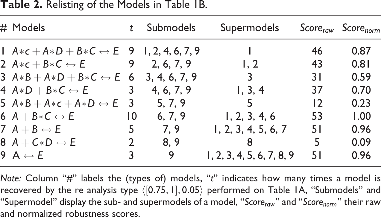
Note: Column “#” labels the (types of) models, “t” indicates how many times a model is recovered by the re analysis type $〈 [0.75, 1],0.05 〉$ performed on Table 1A, “Submodels” and “Supermodel” display the sub- and supermodels of a model, “ $S c o r e_{r a w}$ ” and “ $S c o r e_{n o r m}$ ” their raw and normalized robustness scores.

The columns “Submodels” and “Supermodels” of Table 2 exhibit which models in $M$ are sub- and supermodels of a particular model. For example, model 4 has the submodels 4, 6, 7, and 9 and the supermodels 1, 3, and 4. As detailed in section Preliminaries, every model is both a sub- and a supermodel of itself, which is why every model is listed in both of these columns (in the rows) corresponding to itself. The columns “ $S c o r e_{r a w}$ ” and “ $S c o r e_{n o r m}$ ” provide the raw and normalized fit-robustness scores for each of the models.

To see how these scores are calculated, consider model 4. It has model 6 as a submodel, of which there are 10 instances in $M$ , meaning it receives 10 robustness points from model 6. Model 7 with five instances is another submodel of model 4, hence, supplying another five points. Or, model 1 with nine instances is a supermodel adding nine points to the score. When it comes to counting the sub- and supermodel relations a model bears to itself, we only count different tokens of the model. That is, we subtract two points from the sub- and supermodel relations obtaining among the individual tokens of a model, reflecting the fact that a model token is both a sub- and a supermodel of itself. In total, model 4 has $(10 + 5 + 3 + 9 + 6 + 3 + 3) - 2 = 37$ different token sub- and supermodels in $M$ . More generally, if we denote the sets of sub- and supermodel tokens of model $m_{i}$ by $s u b_{i}$ and $s u p_{i}$ , respectively, the raw robustness score of $m_{i}$ is simply the sum of the cardinalities of $s u b_{i}$ and $s u p_{i}$ minus 2:

s c o r e_{r a w} (m_{i}) = | s u b_{i} | + | s u p_{i} | - 2.

It is evident that, depending on the data and the performed re-analysis type, $s c o r e_{r a w} (m_{i})$ may vary greatly. The raw fit-robustness of $m_{i}$ , when $m_{i}$ is inferred from data $δ$ or by performing $〈 [h, k], l 〉$ , is not comparable to the score of the same model $m_{i}$ when it is inferred from a different δ' or by performing a different re-analysis type $〈 [h^{'}, k^{'}], l^{'} 〉$ . By normalizing the raw scores, we make explicit that fit-robustness is relative to the set $M$ of all models obtained in a re-analysis series. More concretely, the normalized measure $s c o r e_{n o r m} (m_{i})$ amounts to $m_{i}$ ’s raw score divided by the maximum raw score obtained by a model in $M$ . Hence, if $M = {m_{1}, \dots, m_{n}}$ , normalized fit-robustness is this:

s c o r e_{n o r m} (m_{i}) = \frac{s c o r e_{r a w} (m_{i})}{max (s c o r e_{r a w} (m_{1}), \dots, s c o r e_{r a w} (m_{n}))} .

The overall fit-robustness scoring for our example has various notable features. First, model 1, which has the highest consistency and coverage (cf. Table 1B), does not have the highest (FR) score, meaning that (FR) scores do not align with fit. In other words, (FR) is an additional criterion of model selection over and above consistency and coverage. Second, the (FR) score is independent of model complexity. There are complex and simple models with high as well as with low (FR) scores, which corroborates that (FR) has no built-in preference for more or less complex/informative models. Third, the frequency at which a model is returned, while important, is not the sole determinant of the (FR) score and may not even be the decisive one. In the re-analysis series of our example, model 6 is the most frequent one, being returned in 10 of the 36 analyses, and also has the highest (FR) score. But it is clear that frequency alone is not driving the results: The second most frequent models, 1 and 2, are both returned nine times and lose in (FR) score to model 7, returned five times, and to model 9, returned only three times. Fourth, all three models with highest fit-robustness—6, 7, and 9—avoid causal fallacies, as all their causal claims are correct according to the ground truth (3). That means true causal dependencies receive higher (FR) scores than spurious ones. What is more, the highest scoring model, model 6, exactly corresponds to the causal structure (3) used to simulate the data in Table 1A. Thus, (FR) succeeds in selecting the ground truth among all generated models, thereby avoiding both under- and overfitting.

Plainly, though, this example was purposefully selected to introduce and illustrate (FR) on a simple test case. What is needed next is an assessment of whether (FR) achieves its intended purpose when applied to examples not selected for introductory purposes and simplicity, that is, to randomly drawn examples. This is the topic of the next section.

Benchmarking

We extensively benchmarked (FR)-based robustness scoring to determine, first, whether it indeed improves the overall quality of CCM models in discovery contexts featuring random noise and, second, how it fares in contexts with non-random noise. This section reports our results. We first discuss the general setup of our tests and then detail the specifics and results of the tests with random and non-random noise, respectively. We executed all tests both on crisp-set and fuzzy-set data. For brevity, our subsequent discussion focuses on the crisp-set tests, which, overall, turned out to be less favorable to (FR)-based robustness scoring. The results of the fuzzy-set tests are presented in the Online Appendix. The Online Supplementary Material moreover supplies separate replication scripts for all tests.

General Test Setup

To determine whether selecting models based on high (FR) scores improves or diminishes the overall model quality, we contrast it with standard model selection approaches. More specifically, we process data by means of CNA and select sets $S$ of models using the following four approaches: The first, which we label FRscore, selects the models with highest (FR) scores resulting from the re-analysis type $〈 [0.7, 1],0.1 〉$ ; the second, MaxFit, selects the models with the highest products of consistency and coverage (con-cov products) generated by the maximal consistency and coverage setting in the interval [0.7, 1] actually producing a model; the third, Conv0.8, selects the models with highest con-cov products generated at the conventional threshold setting $〈 0.8, 0.8 〉$ ; and the fourth, Conv0.75, selects the models with highest con-cov products generated at the conventional setting $〈 0.75, 0.75 〉$ . In the selected sets $S$ of top-scoring models, we do not merely include the models with maximal (FR) scores and con-cov products, respectively, but the models at or above the 98th percentile of (FR) scores and con-cov products.

To determine the quality of the selected models in $S$ , we have to compare them with the ground truth, meaning we have to know the data-generating causal structures. As these are typically unknown in real-life data, we run our tests on simulated data. More specifically, we conduct inverse searches, which reverse the order of normal causal discovery. An inverse search comprises three main steps: (1) a causal structure $Δ$ is drawn (as ground truth), (2) data $δ$ are simulated from $Δ$ , featuring varying deficiencies (e.g., different types of noise), and (3) $δ$ is processed by the benchmarked method in order to check whether its output meets a tested benchmark criterion.

We test the model sets $S$ against three increasingly stringent benchmark criteria: first, whether $S$ is fallacy-free; second, whether $S$ contains a correct model; and third, to what degree correct models in $S$ completely reflect the ground truth. A set $S$ is fallacy-free iff it does not entail a causal claim that is false of the ground truth $Δ$ (i.e., no false positive). Clarifying when $S$ satisfies that condition calls for some preliminary remarks on the phenomenon of model ambiguities.

It is a frequent phenomenon in all methodological frameworks that empirical data underdetermine their own causal modeling to the effect that multiple models account for them equally well (e.g., Baumgartner and Thiem 2017; Eberhardt 2013; Spirtes et al. 2000:59-72). In cases of such ambiguities, CCMs output all data-fitting models (and leave the disambiguation up to the analyst). It follows that, if a CCM issues multiple models, it is not thereby implying that all of these models correspond to the ground truth but only that (at least) one of them does, and that—based on the available evidence—it is undetermined which one exactly. The same holds if one of FRscore, MaxFit, Conv8.0, or Conv0.75 selects multiple models, that is, if $S = {m_{1}, m_{2}, \dots, m_{n}}$ with $n > 1$ . Such a result is to be interpreted disjunctively: The data-generating structure is:

m_{1} OR m_{2} OR ... OR m_{n} .

A disjunction is true iff at least one disjunct is true; and conversely, it is false iff all disjuncts are false. Hence, in order for a set of models $S$ to be fallacy-free, it must not be the case that all models in $S$ are false. This can be satisfied in two ways: Either (i) $S$ is empty (e.g., because chosen fit thresholds cannot be met) or (ii) $S$ contains at least one model $m_{i}$ that is correct of the ground truth $Δ$ , which is the case iff $m_{i}$ is a submodel of $Δ$ . So, $S$ satisfies our first benchmark criterion iff it satisfies conditions (i) or (ii). The reader may wonder why we test a benchmark that can, in principle, be passed by a trivial method producing empty outputs by default. The reason is that such a method would be entirely uninformative, which would be visible in its failing our third, completeness, benchmark; but an empty output produced by a method that does not fail on completeness is a valuable piece of information entailing that the data do not warrant any causal conclusions. The capacity to abstain from drawing causal inferences when no such inferences are warranted is a crucial methodological asset that deserves to be benchmarked.

In light of that specification of fallacy-freeness, our second benchmark criterion is straightforwardly clarified. It focuses on non-empty sets $S$ only and checks whether condition (ii) is satisfied, meaning whether $S$ actually contains at least one model $m_{i}$ that is a submodel of $Δ$ , and thus correct. That is, while an empty set $S$ passes the first benchmark, it does not pass the second.¹⁰

Finally, our third benchmark criterion addresses the fact that the correctness of a model does not entail anything about its informativeness. In other words, of two different models that are both submodels of the ground truth $Δ$ , one can be more complex than the other and, hence, reveal $Δ$ more completely. It is clear that the more complete correct model is preferable. Hence, of two approaches that select correct models equally reliably, the one whose selected models are more complete, on average, is preferable. The completeness benchmark measures the degree to which the correct models in $S$ exhaustively reveal $Δ$ . More specifically, the completeness criterion amounts to the ratio of the complexity of the most complex correct model in $S$ to the complexity of $Δ$ , where complexity of a model is, again, understood as the number of exogenous factor values contained in it.¹¹ That is, contrary to the first and second benchmarks, which can only be passed or not, the third benchmark can be passed by degree.

Random Noise

In a first series of tests, we compare the performance of FRscore, MaxFit, Conv0.8, and Conv0.75 on the above benchmarks when the analyzed data feature randomly distributed noise, meaning randomly drawn cases incompatible with the ground truth. That performance depends on various parameters, such as the complexity of the ground truth, the sample size, or the noise ratio. To vary these parameters (to some degree), we set up 12 different test types simulating data $δ$ from randomly generated ground truths $Δ$ comprising values of some (not necessarily all) of the crisp-set factors in $F = {A, B, C, D, E, F}$ . The 12 test types differ insofar as each of them realizes one logically possible variation of the following parameters: (1) number of outcomes in $Δ$ , with a variation between one and two outcomes; (2) sample size multiplier, with a variation between one and three (i.e., one and three cases per configuration); and (3) ratio of cases in $δ$ replaced by cases incompatible with $Δ$ , with a variation between 0.05, 0.15, and 0.25. For transparency, the 12 test types are listed and numbered in Table 3. In test #6, for example, we generate ground truths $Δ$ with two outcomes and simulate data $δ$ from each of them by, first, generating an ideal data set $δ^{i d}$ comprising one case per configuration and by, second, replacing 15 percent of the cases in $δ^{i d}$ by randomly drawn cases incompatible with $Δ$ . Importantly, in all of these tests, each case of $δ^{i d}$ has equal probability of being replaced by an incompatible case and all incompatible cases have equal probability of being drawn.

Table 3.

The 12 Test Types of the Random Noise Series.

Test Type	No. of Outcomes in $Δ$	Sample Size Multiplier	Ratios of Incompatible Cases
1	1	1	0.05
2	2	1	0.05
3	1	3	0.05
4	2	3	0.05
5	1	1	0.15
6	2	1	0.15
7	1	3	0.15
8	2	3	0.15
9	1	1	0.25
10	2	1	0.25
11	1	3	0.25
12	2	3	0.25

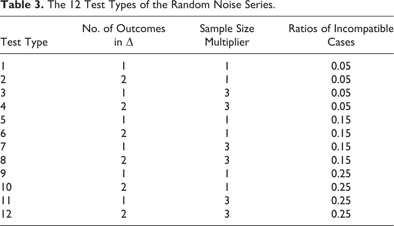
One particular test trial, that is, one instance of a test type, consists in a data set simulated according to the parameters of that type being sequentially processed by FRscore, MaxFit, Conv0.8, and Conv0.75. The resulting four sets of selected models are then benchmarked for fallacy-freeness, correctness, and completeness. 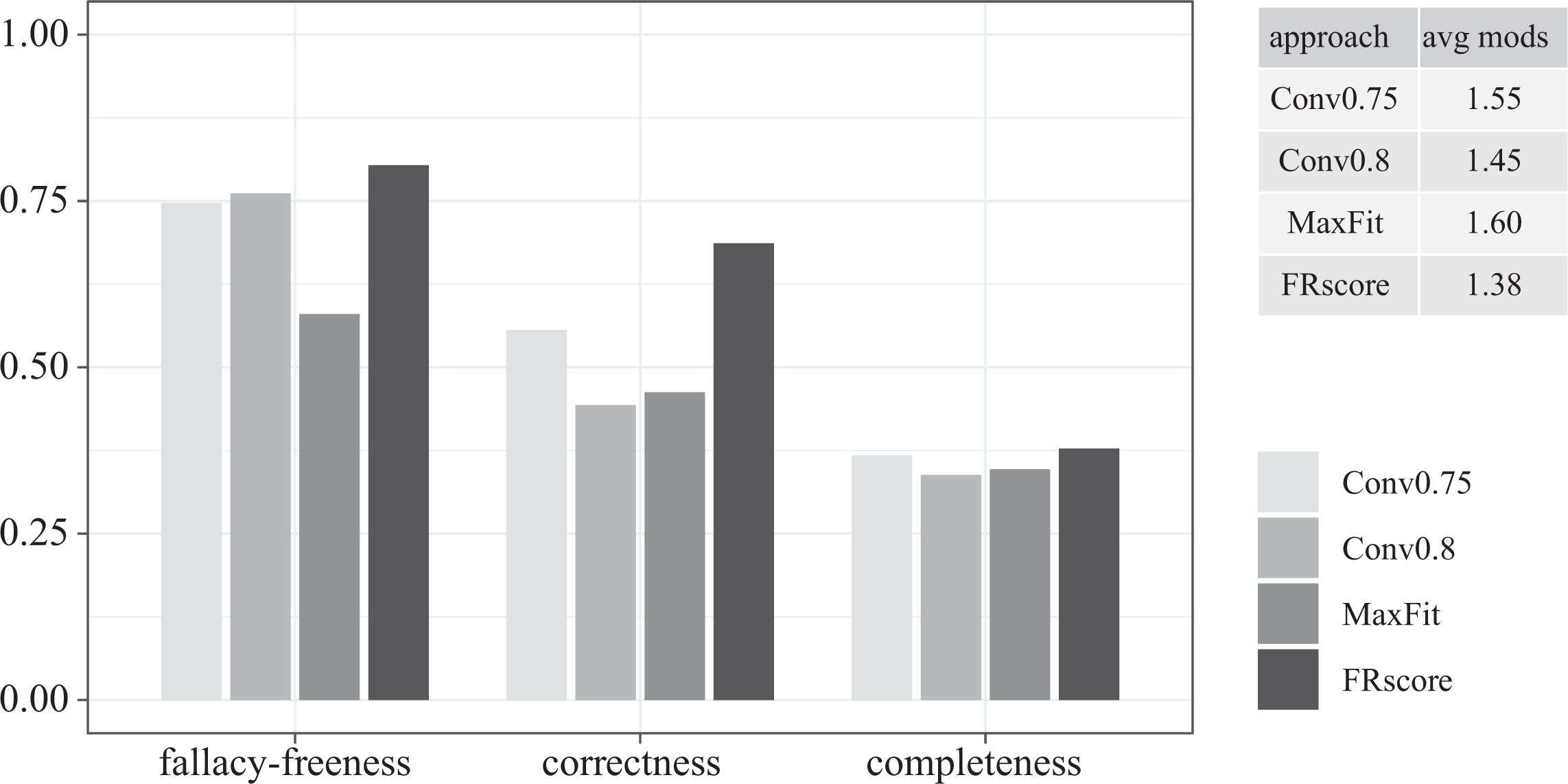To get a statistically reliable performance assessment, we run 1,000 trials of each test type, yielding a total of $12 \times 1, 000 = 12, 000$ trials. The bar chart in Figure 2 plots the corresponding benchmark scores for the four selection approaches averaged over all 12,000 trials.

Figure 2.

Benchmark scores averaged over all 12,000 trials of the random-noise test series. The top-right table provides the average number of models per trial selected by an approach.

These averaged results show that, across all different $Δ$ complexities, sample sizes, and ratios of incompatible cases, FRscore significantly outperforms the other approaches on the correctness benchmark. While only including 1.38 models in $S$ per trial, on average, FRscore finds a correct model in 69 percent of the trials. The other approaches include over 1.45 models in $S$ , which comprises a correct model in only 56 percent (Conv0.75), 44 percent (Conv0.8), and 46 percent (MaxFit) of the trials. FRscore also scores highest on completeness, which demonstrates that the correct models singled out by FRscore are not less informative than the models issued by the other approaches. At the same time, the overall low completeness scores indicate that, in the presence of up to 25 percent of cases incompatible with $Δ$ , CNA can only uncover a little over a third of $Δ$ —which, roughly, corresponds to the completeness restrictions Arel-Bundock (2019) has recently exhibited for QCA. Finally, FRscore likewise has an edge over the other approaches on the fallacy-freeness benchmark, which, to recall, can be passed either by a correct or by an empty output. FRscore avoids a causal fallacy in 80 percent of the trials (with 11 percent empty outputs), as opposed to a score of 75 percent (19 percent empty) by Conv0.75, 76 percent (32 percent empty) by Conv0.8, and 58 percent (12 percent empty) by MaxFit. This shows once again that, while the false positive risk for (non-maximal) conventional threshold settings is manageable, maximizing model fit is an unsuitable approach to model selection.

To set these results into proper perspective, the three bar charts in Figure 3 break them down by the parameters varied in our 12 test types. The first chart shows that FRscore scores highest on correctness at all noise ratios—by a particularly large margin in high noise scenarios. While Conv0.75 and Conv0.8 reach decent scores on fallacy-freeness even in the tests with 25 percent incompatible cases, they only find a correct model in, respectively, 20 percent and 12 percent of the trials, meaning that they mostly issue no model at all, whereas FRscore still recovers a correct model in 40 percent of the trials. At the same time, the most cautious approach, Conv0.8, which typically abstains from drawing any causal inferences when processing the most noisy data, avoids causal fallacies in 73 percent of the trials, while FRscore only reaches 69 percent on fallacy-freeness. That is, in the tests with 25 percent incompatible cases, FRscore comes with a slightly higher false positive risk than Conv0.8, which, however, is counterbalanced by a more than three times higher prospect of actually being rewarded by the recovery of a correct model. While Conv0.8 has an advantage on completeness in the tests with only 5 percent noise, the models selected by FRscore are the most complete ones in all other tests.

Figure 3.

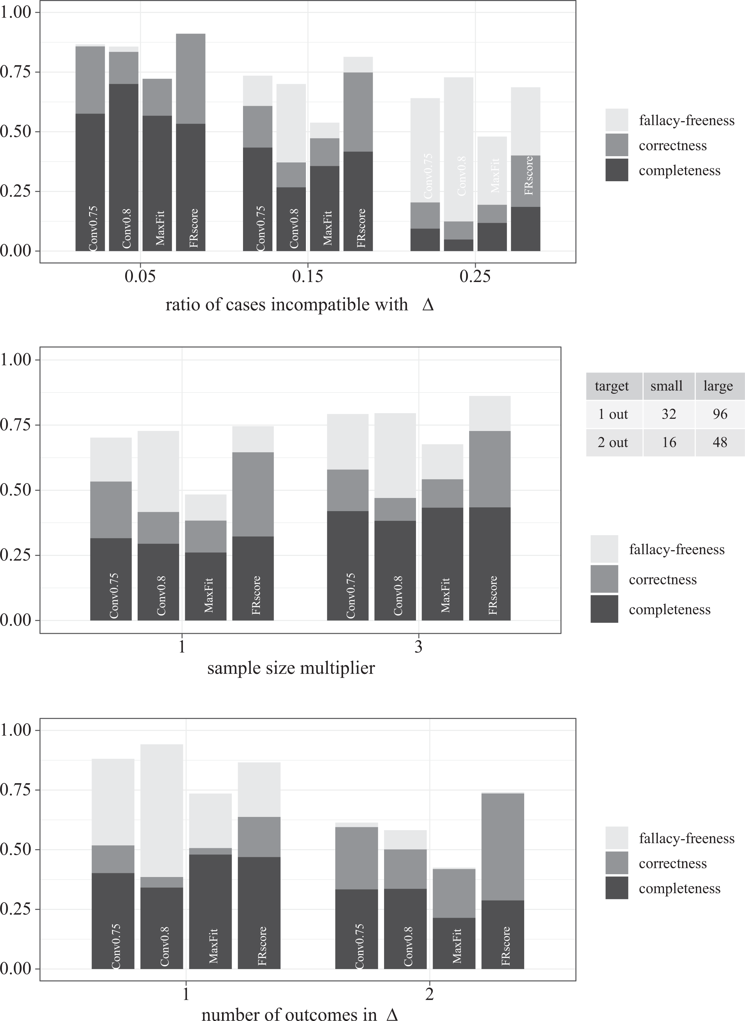
Benchmark scores broken down by the ratio of cases incompatible with $Δ$ (top), the sample size multiplier (middle), and the number of outcomes in $Δ$ (bottom).

The second chart in Figure 3 shows a similar edge of FRscore over the other approaches as regard to correctness in all sample sizes. As is to be expected, all benchmark scores are better in the larger sample sizes. MaxFit is by far the most unreliable approach, in particular, in small-sized data: While Conv0.75, Conv0.8, and FRscore avoid causal fallacies in over 70 percent of the trials, MaxFit misfires in half of the trials. Finally, the third chart in Figure 3 plots the benchmarks against the complexity of $Δ$ . These results give rise to various questions. For instance, if $Δ$ has two outcomes, the scores on fallacy-freeness are significantly lower for all selection approaches. That is, the complexity of the data-generating structure considerably increases the false positive risk. At the same time, both Conv0.75 and FRscore have higher correctness scores if $Δ$ has two outcomes. We do not have explanations for either of these findings. They demonstrate that the interdependence between the complexity of the data-generating structure and the reliability of corresponding CCM outputs is in need of further scrutiny.

Non-random Noise

Of course, cases incompatible with the data-generating structure may not be equally probable. Certain types of measurement error may more frequently occur than others or unmeasured variation of latent causes may confound the data with a bias. In order to also assess the performance of FRscore in non-random noise scenarios, we compare it with MaxFit, Conv0.8, and Conv0.75 in a second series of three additional classes of tests. Tests in class I are set up analogously to our previous tests, that is, ground truths $Δ$ are randomly generated from the set of crisp-set factors $F = {A, B, C, D, E, F}$ , and cases in ideal data are replaced by cases incompatible with $Δ$ . Now however, incompatible cases are not selected with equal probability but such that 70 percent of them are identical. This shall simulate discovery contexts in which certain types of measurement error are systematically repeated. In order for this bias to be manifest in the data, we keep the ratio of incompatible cases constant at 20 percent of the sample size. As before, we vary the number of outcomes in $Δ$ and the sample size multipliers, yielding a total of four test types in class I (see Table 4).

Table 4.

The Seven Test Types of the Non-random Noise Series.

Test Type	No. of Outcomes in $Δ$	Sample Size Multiplier	Noise
Ⅰ1 Ⅰ2 Ⅰ3 Ⅰ4	1 2 1 2	1 1 3 3	20% incompatible cases with 70% identicals
Ⅱ1 Ⅱ2	1 2	1 1	One varying latent cause
Ⅲ1	2	1	One varying latent common cause

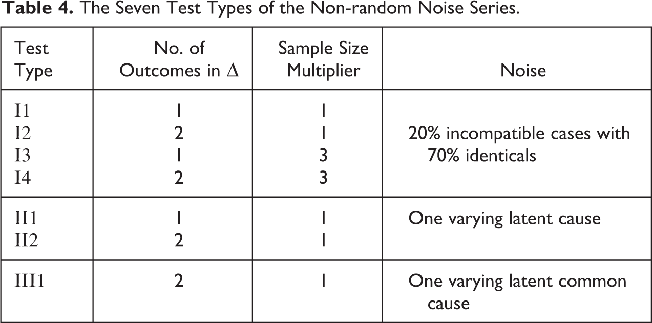
Tests of classes II and III are set up differently. They do not simulate noise due to measurement error but noise induced by an uncontrolled variation in latent causes. Instead of replacing cases in ideal data with incompatible ones, we now draw ground truths and generate ideal data from which we then eliminate columns corresponding to causally relevant factors. Tests in classes II and III differ in the severity of the resulting data confounding. In class II, ground truths are built from the factors in $F$ with both one and two outcomes, and one randomly selected causally relevant factor is eliminated from the data. In class III, we only generate two-outcome structures with at least one common cause of those two outcomes; we then eliminate that common cause from the data, which yields a strong spurious dependence of the two outcomes. To ensure that the data contain causally irrelevant factors on a regular basis, as in all the other test types, we add an additional factor to the set from which ground truths are drawn: $F' = {A, B, C, D, E, F, G}$ . As the tests in classes II and III merely eliminate columns from ideal data without inserting any incompatible cases, varying the sample size multiplier cannot yield data with varying difference-making evidence.¹² Hence, we keep the sample size multiplier constant in these two test classes. Table 4 provides an overview over all seven test types of this test series.

As before, we run 1,000 trials of each test type. The bar charts in Figure 4 plot the benchmark scores averaged over all trials in each test class. The main finding is that FRscore only has a clear edge over the other selection approaches in the tests of class I. While the systematicity of the measurement error drags down the overall performance of CNA significantly (as it would for any method), it still holds that FRscore selects a correct model in 50 percent of the trials, which is about twice as much as the other approaches. Moreover, its models are most complete—although at a low level of 15 percent—and it likewise avoids causal fallacies most frequently (54 percent). But the low scores of all approaches on the fallacy-freeness benchmark exhibit that systematic measurement error is not reliably detected by CNA, which, as a result, misfires where it should abstain from drawing any causal inference.

Figure 4.

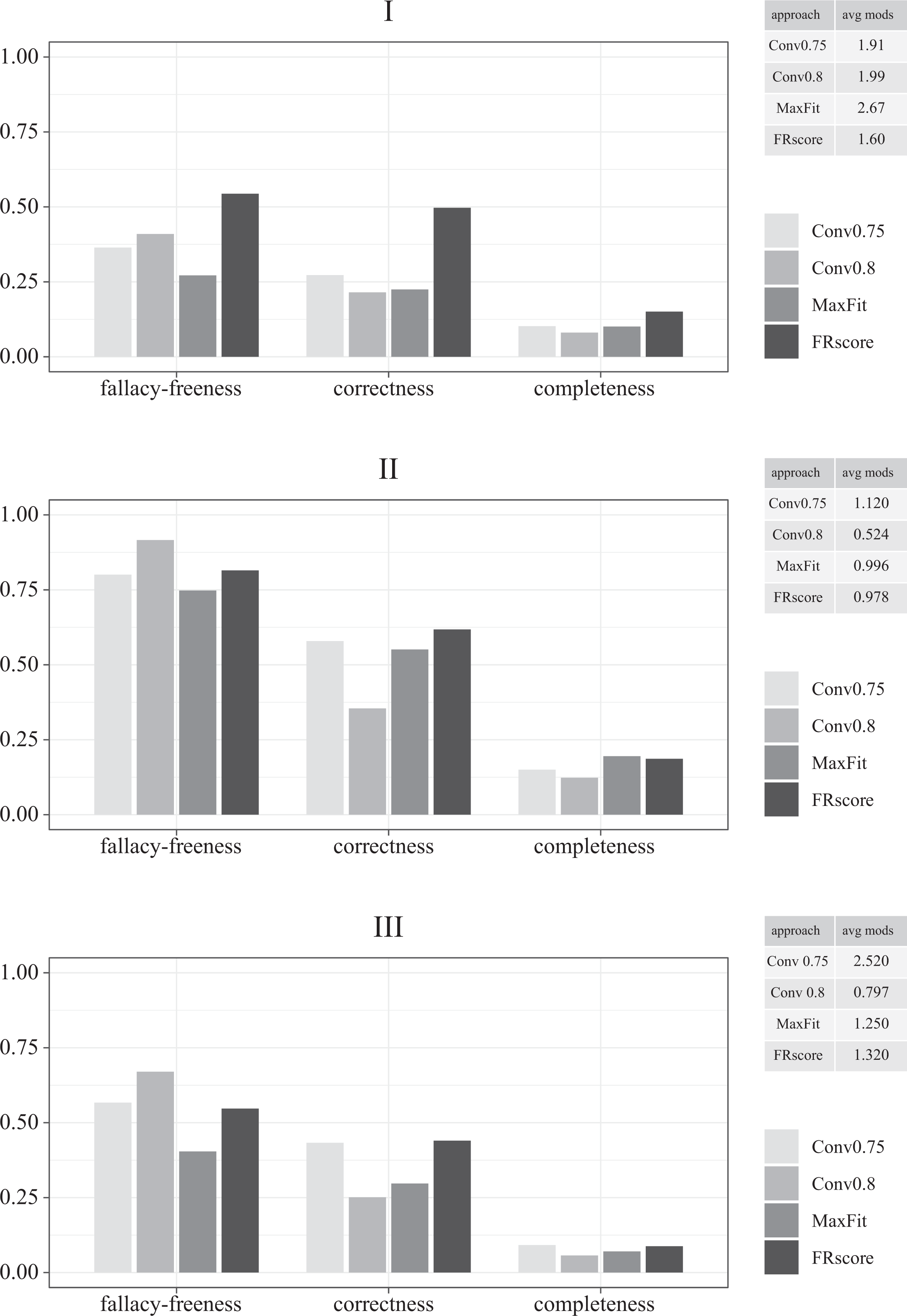
Benchmark scores averaged over all trials in classes I (top), II (middle), and III (bottom) of the non-random-noise series.

This changes in the tests of class II. Conv0.8 reliably detects noise induced by a variation of latent causes and avoids causal fallacies in 92 percent of the trials—mostly by abstaining from drawing an inference. Although beaten by Conv0.8 on fallacy-freeness, FRscore (62 percent) scores better than the other approaches on correctness. When it comes to completeness, MaxFit scores highest (20 percent). The results in the tests of class III are similar, albeit at a significantly lower level. When a common cause of two observed factors is unmeasured, Conv0.8 avoids fallacies in 67 percent of the trials. But also in these tests, FRscore scores highest on correctness (44 percent). While Conv0.75 (43 percent) recovers almost as many correct models as FRscore, it outputs nearly twice as many models per trial. Finally, there is a tie between Conv0.75 and FRscore on the completeness benchmark, both recovering 9 percent of the ground truth, on average. The Online Appendix provides additional plots breaking down those average scores by the varied parameters.

Overall, while FRscore performs best on all benchmarks in the tests of class I, it only scores higher than the other selection approaches on the correctness benchmark in classes II and III. If there are varying latent causes, there is a certain danger that FRscore is not cautious enough and produces false positives that could be avoided by a more cautious selection approach as Conv0.8.

Conclusion

This article has shown that maximizing consistency and coverage thresholds in configurational causal modeling is a highly unreliable practice, even in the presence of only mild degrees of noise. Maximizing model fit induces CCMs to overfit at unacceptably high rates, which various critics of CCMs have justifiably pointed out. The non-maximal threshold settings that have evolved by convention over the years alleviate the overfitting danger considerably—however, at the price of recovering data-generating structures less completely than would be possible based on the available evidence (i.e., underfitting) or of abstaining from drawing causal inferences altogether. Overall, there is a clear need for complementing standard criteria of model fit by further criteria of model selection.

To this end, we developed a criterion of fit-robustness which measures the degree to which a model overlaps in its causal ascriptions with other models inferred from re-analyzing data at systematically varied consistency and coverage thresholds. The more overlap, the higher the (FR) score. We argued that, contrary to robustness measures customary in statistical methods, which reward model invariance, (FR) does justice to the fact that CCMs are expressly built to mirror cross-case variation. (FR) allows for ample variation among output models, as long as they are sub- or supermodels of one another and, hence, do not make idiosyncratic causal ascriptions.

Contrary to recent robustness considerations in the methodological literature on CCMs, (FR) is straightforwardly computable based on the submodel relation, and we implemented it as an explicit R function. We extensively benchmarked model selection based on (FR) in two test series, one with random and one with non-random noise, comparing it to standard approaches of model selection. If noise is randomly distributed, (FR) scoring reduces the false positive risk by 5 to 22 percentage points, depending on the alternative approach it is contrasted with, and it increases the chances that a correct model—which is as complete about the ground truth as possible—is actually returned by 13 to 25 points. To top it off, this maximization of correctness coupled with a minimization of the false positive risk is achieved while only issuing 1.38 models per trial, which amounts to the lowest ambiguity ratio of all selection approaches. Hence, if there is reason to assume that noise is randomly distributed, selecting CCM models based on the measure of fit-robustness developed in this article is unequivocally recommendable.

By contrast, in discovery contexts featuring non-randomly distributed noise, for example, induced by systematic measurement error or confounding, the overall performance of CCMs is so severely hampered that using a standard selection approach, which cautiously abstains from drawing any causal inferences if noise ratios are too high, might be the safer bet. But even in non-random noise scenarios, analysts willing to take a risk are well advised to select models based on the robustness measure developed in this article because, although it does not minimize the false positive risk, it still maximizes the chances of actually finding a correct model.

Supplemental Material

Supplemental Material, sj-zip-1-smr-10.1177_0049124120986200 - Robustness and Model Selection in Configurational Causal Modeling

Supplemental Material, sj-zip-1-smr-10.1177_0049124120986200 for Robustness and Model Selection in Configurational Causal Modeling by Veli-Pekka Parkkinen and Michael Baumgartner in Sociological Methods & Research

Footnotes

Acknowledgments

The authors would like to thank the audience at CLMPTS 2019 in Prague, where an early version of this article was presented, as well as two anonymous referees for their helpful comments and suggestions. They also wish to thank the Toppforsk program of the University of Bergen and the Trond Mohn Foundation for financial support.

Declaration of Conflicting Interests

The author(s) declared no potential conflicts of interest with respect to the research, authorship, and/or publication of this article.

Funding

The author(s) disclosed receipt of the following financial support for the research, authorship, and/or publication of this article: The authors received funding from the Trond Mohn Foundation, grant ID 811866.

ORCID iD

Veli-Pekka Parkkinen

Michael Baumgartner

Supplemental Material

Supplemental material for this article is available online.

Notes

References

Ambühl

Mathias

Baumgartner

Michael

. 2020. cnaOpt: Optimizing Consistency and Coverage in Configurational Causal Modeling. R Package Version 0.2.0. https://cran.r-project.org/package=cnaOpt. Retreived 11 February, 2021.

Arel-Bundock

Vincent

. 2019. “The Double Bind of Qualitative Comparative Analysis.” Sociological Methods & Research. doi:10.1177/0049124119882460.

Baumgartner

Michael

Ambühl

Mathias

. 2020. “Causal Modeling with Multi-value and Fuzzy-set Coincidence Analysis.” Political Science Research and Methods 8(3):526–42. doi:10.1017/psrm.2018.45.

Baumgartner

Michael

Falk

Cristoph

. 2019. “Boolean Difference-making: A Modern Regularity Theory of Causation.” The British Journal for the Philosophy of Science. doi:10.1093/bjps/axz047.

Baumgartner

Michael

Thiem

Alrik

. 2017. “Model Ambiguities in Configurational Comparative Research.” Sociological Methods & Research 46(4):954–87.

Baumgartner

Michael

Thiem

Alrik

. 2020. “Often Trusted But Never (Properly) Tested: Evaluating Qualitative Comparative Analysis.” Sociological Methods & Research 49(2):279–311. doi:10.1177/0049124117701487.

Braumoeller

Bear F.

2015. “Guarding against False Positives in Qualitative Comparative Analysis.” Political Analysis 23(4):471–87.

Cooper

Barry

Glaesser

Judits

. 2016. “Exploring the Robustness of Set Theoretic Findings From a Large N fsQCA: An Illustration from the Sociology of Education.” International Journal of Social Research Methodology 19(4):445–59.

Cronqvist

Lasse

Berg-Schlosser

Dirk

. 2009. “Multi-value QCA (mvQCA).” Pp. 69–86 in Configurational Comparative Methods: Qualitative Comparative Analysis (QCA) and Related Techniques, edited by Rihoux

Ragin

C. C.

. London, England: Sage.

10.

Dusa

Adrian

. 2018. “Consistency Cubes: A Fast, Efficient Method for Exact Boolean Minimization.” The R Journal 10(2):357–70.

11.

Eberhardt

Frederick

. 2013. “Experimental Indistinguishability of Causal Structures.” Philosophy of Science 80(5):684–96.

12.

Gelman

Andrew

Hill

Jennifer

. 2007. Data Analysis Using Regression and Multilevel/Hierarchical Models. Cambridge, England: Cambridge University Press.

13.

Graßhoff

Gerd

May

Michael

. 2001. “Causal Regularities.” Pp. 85–114 in Current Issues in Causation, edited by Spohn

Ledwig

Esfeld

. Paderborn, Germany: Mentis.

14.

Hug

Simon

. 2013. “Qualitative Comparative Analysis: How Inductive Use and Measurement Error Lead to Problematic Inference.” Political Analysis 21(2):252–65.

15.

Krogslund

Chris

Choi

Donghuyn D.

Poertner

Mathias

. 2015. “Fuzzy Sets on Shaky Ground: Parameter Sensitivity and Confirmation Bias in fsQCA.” Political Analysis 23(1):21–41.

16.

Lemmon

E. John

. 1965. Beginning Logic. London, England: Chapman & Hall.

17.

Lewis

David

. 1973. “Causation.” Journal of Philosophy 70:556–67.

18.

Lucas

Samuel R.

Szatrowski

Alisa

. 2014. “Qualitative Comparative Analysis in Critical Perspective.” Sociological Methodology 44(1):1–79.

19.

Mackie

John L.

1974. The Cement of the Universe. A Study of Causation. Oxford, England: Clarendon Press.

20.

Ragin

Charles.C.

2006. “Set Relations in Social Research: Evaluating Their Consistency and Coverage.” Political Analysis 14:291–310.

21.

Ragin

Charles C.

2008. Redesigning Social Inquiry: Fuzzy Sets and Beyond. Chicago: University of Chicago Press.

22.

Rohlfing

Ingo

. 2015. “Mind the Gap: A Review of Simulation Designs for Qualitative Comparative Analysis.” Research & Politics 2(4):1–4.

23.

Schneider

Carsten Q.

Wagemann

Claudius

. 2012. Set-theoretic Methods for the Social Sciences: A Guide to Qualitative Comparative Analysis. Cambridge: Cambridge University Press.

24.

Skaaning

Svend-Erik

. 2011. “Assessing the Robustness of Crisp-set and Fuzzy-set QCA Results.” Sociological Methods & Research 40(2):391–408.

25.

Spirtes

Peter

Glymour

Clarke

Scheines

Richard

. 2000. Causation, Prediction, and Search. Cambridge: MIT Press.

26.

Suppes

Peter

. 1970. A Probabilistic Theory of Causality. Amsterdam: North Holland.

27.

Thiem

Alrik

. 2014a. “Membership Function Sensitivity of Descriptive Statistics in Fuzzy-set Relations.” International Journal of Social Research Methodology 17(6):625–42.

28.

Thiem

Alrik

. 2014b. “Unifying Configurational Comparative Methods: Generalized-set Qualitative Comparative Analysis.” Sociological Methods & Research 43(2):313–37.

29.

Thiem

Alrik

Baumgartner

Michael

. 2016. “Modeling Causal Irrelevance in Evaluations of Configurational Comparative Methods.” Sociological Methodology 46:345–57. doi:10.1177/0081175016654736.

30.

Thiem

Alrik

Spöhel

Reto

Dusa

Adrian

. 2016. “Enhancing Sensitivity Diagnostics for Qualitative Comparative Analysis: A Combinatorial Approach.” Political Analysis 24(1):104–20.

Supplementary Material

Please find the following supplemental material available below.

For Open Access articles published under a Creative Commons License, all supplemental material carries the same license as the article it is associated with.

For non-Open Access articles published, all supplemental material carries a non-exclusive license, and permission requests for re-use of supplemental material or any part of supplemental material shall be sent directly to the copyright owner as specified in the copyright notice associated with the article.

0.05 MB

0.00 MB