Optimizing Consistency and Coverage in Configurational Causal Modeling

Abstract

Consistency and coverage are two core parameters of model fit used by configurational comparative methods (CCMs) of causal inference. Among causal models that perform equally well in other respects (e.g., robustness or compliance with background theories), those with higher consistency and coverage are typically considered preferable. Finding the optimally obtainable consistency and coverage scores for data $\text{δ}$ , so far, is a matter of repeatedly applying CCMs to $\text{δ}$ while varying threshold settings. This article introduces a procedure called ConCovOpt that calculates, prior to actual CCM analyses, the consistency and coverage scores that can optimally be obtained by models inferred from $\text{δ}$ . Moreover, we show how models reaching optimal scores can be methodically built in case of crisp-set and multi-value data. ConCovOpt is a tool, not for blindly maximizing model fit, but for rendering transparent the space of viable models at optimal fit scores in order to facilitate informed model selection—which, as we demonstrate by various data examples, may have substantive modeling implications.

Introduction

Over the past three decades, different variants of configurational comparative methods (CCMs) have gradually been added to the tool kit for causal data analysis in many disciplines, ranging from social and political science to business administration, evaluation science, and on to public health and psychology. CCMs are designed to investigate causal structures featuring conjunctural causation and equifinality, which tend to prevent pairwise (linear) dependencies among analyzed variables and, hence, induce problems for many standard methodological frameworks. While other methods search for causal relations as characterized by counterfactual or probabilistic theories of causation (e.g., Lewis 1973; Suppes 1970), CCMs trace causation as defined in the tradition of Mackie’s (1974) INUS theory. ¹ CCMs do not quantify effect sizes but place a Boolean ordering on sets of causes by grouping their elements conjunctively, disjunctively, and sequentially. And unlike the models produced by many other methods, CCM models do not relate variables to one another but concrete values of variables (cf. Thiem et al. 2016).

The most well-known CCM is Qualitative Comparative Analysis (QCA; Cronqvist and Berg-Schlosser 2009; Ragin 1987, 2008). Coincidence Analysis (CNA) is a more recent addition to the family of CCMs (Baumgartner 2009; Baumgartner and Ambühl 2020). There are various differences between QCA and CNA—in the underlying methodological principles, in the implemented algorithms, or in the search targets—but also important commonalities. Both methods process configurational data featuring crisp-set, fuzzy-set, or multi-value variables (Thiem 2014), which are called factors in CCM jargon. They both exploit relations of sufficiency and necessity for causal inference and output models accounting for the values taken by endogenous factors in terms of redundancy-free Boolean functions of exogenous factor values. And they share two of their core parameters of model fit, which constitute the topic of this article: consistency and coverage (Ragin 2006). Informally, consistency reflects the degree to which the behavior of an outcome obeys a corresponding sufficiency or necessity relationship or a whole model, whereas coverage reflects the degree to which a sufficiency or necessity relationship or a whole model accounts for the behavior of the corresponding outcome. What counts as acceptable scores on these parameters is defined in threshold settings determined by the analyst prior to the application of QCA or CNA.

Among causal models that perform equally well with respect to other criteria, for example, robustness and compliance with case knowledge or background theories, the ones with the higher aggregate of consistency and coverage are considered preferable. This raises the question of how to systematically find the models with optimal consistency and coverage. Currently, neither the procedural protocols of QCA nor of CNA have answers to that question on offer. Rather, optimizing consistency and coverage is a matter of repeatedly running QCA and CNA on the data while varying relevant thresholds and comparing the fit scores of resulting models. Such a trial-and-error approach is neither guaranteed to recover all consistency and coverage optima, of which there may be many, nor is it efficient, as it may require a multitude of data re-analyses. Variations in the thresholds may induce substantive changes in the issued models as well as in their fit scores. These changes may not be proportional to the threshold variations. That is, higher thresholds are not guaranteed to produce models with higher aggregates of consistency and coverage. In consequence, a wide range of threshold settings may have to be searched in fine-grained steps.

This article shows that it is possible to identify optimal consistency and coverage scores of CCM models inferable from data $\text{δ}$ independently of actually applying CCMs to $\text{δ}$ . We introduce an explicit procedure, called ConCovOpt, that calculates all consistency and coverage optima for $\text{δ}$ , within certain computational limitations, prior to CCM analyses. ConCovOpt is complemented by a second procedure, called DNFbuild, that purposefully builds models reaching optimal scores for crisp-set and multi-value data. For these data types, models are hence guaranteed to exist at the consistency and coverage optima. ConCovOpt can also be applied to fuzzy-set data, in which case optimas amount to upper bounds that cannot possibly be outperformed by actual models, but there is no guarantee that models de facto exist at those bounds. The upper bounds, thus, constrain the interval of threshold settings within which optimal actual models must be searched.

ConCovOpt is a tool, not for blindly maximizing model fit, but for systematically exploring the space of viable models with optimal fit. Sometimes, optimally fitting models will turn out to be the best models overall, while sometimes optimizing consistency and coverage is only possible at the price of overfitting or of compromising on robustness or compliance with background theories or case knowledge. Choosing the best model(s) among all viable models, which may be numerous (Baumgartner and Thiem 2017), is a delicate task that requires balancing various criteria. Consistency and coverage are only two of those criteria. But, independently of whether the analyst wants to anchor that choice in the data only or additionally draw on external sources of information, making an informed choice presupposes that the whole model space is brought to the analyst’s attention. The purpose of ConCovOpt is to contribute to that objective.

This article is organized as follows. The second section reviews some conceptual preliminaries. In the third section, ConCovOpt is presented using a simple crisp-set data example. The fourth section applies it to large-N data. DNFbuild is introduced in the fifth section on the basis of multi-value data; and a fuzzy-set application is discussed in the sixth section. Finally, the seventh section puts ConCovOpt into proper methodological perspective. We implemented ConCovOpt and DNFbuild in an R package called cnaOpt (Ambühl and Baumgartner 2020b), which is an add-on to the cna package (Ambühl and Baumgartner 2020a) and is extensively used in the replication script available in the Online Supplementary Material (which can be found at http://smr.sagepub.com/supplemental/).

Conceptual Preliminaries

We begin by introducing some conceptual and notational preliminaries of our ensuing discussion. As indicated above, CCMs study Boolean dependence relations between factors taking on specific values. Factors represent categorical properties that partition sets of units of observation (cases) either into two sets, in case of binary properties, or into more than two (but finitely many) sets, in case of multi-value properties. Factors representing binary properties can be crisp-set ( $cs$ ) or fuzzy-set ( $fs$ ); the former typically take on 0 and 1 as possible values, whereas the latter can take on any (continuous) values from the unit interval. Factors representing multi-value properties are called multi-value ( $mv$ ) factors; they can take on any of an open (but finite) number of non-negative integers as possible values. Values of a $cs$ or $fs$ factor X are often interpreted as membership scores in the set of cases exhibiting the property represented by X, while the values of an $mv$ factor Y designate the particular way in which the property represented by Y is exemplified.

As the explicit “Factor $=$ value” notation yields convoluted syntactic expressions with increasing model complexity, we subsequently use—whenever possible—a shorthand notation that is conventional in Boolean algebra and CCM modeling: Membership in a set is expressed by italicized upper case and non-membership by lower case Roman letters. Hence, in case of $cs$ and $fs$ factors, we normally write “X” for X=1 and “x” for X=0. In case of $mv$ factors and within explicit definitions, value assignments are always written out, using the “Factor $=$ value” notation; that is, we write “Y= $\nu$ ” for factor Y taking the value $\nu$ .

CCM models may feature all the standard Boolean operations: negation $\neg X$ (“not X”), conjunction X $\ast$ Y (“X and Y”), disjunction $X+Y$ (“X or Y”), implication $X\to Y$ (“If X, then Y”), and equivalence $X\leftrightarrow Y$ (“X if, and only if, Y”). In case of $cs$ and $mv$ factors, these operations are given a rendering in classical logic (see, e.g., Lemmon 1965, for a canonical introduction). In case of $fs$ factors, Boolean operations are rendered in fuzzy logic: negation $\neg X$ amounts to $1-X$ , conjunction X $\ast$ Y to $\text{min}(X,Y)$ , disjunction $X+Y$ to $\text{max}(X,Y)$ , an implication $X\to Y$ is taken to express that the membership score in X is smaller or equal to Y (i.e. $X\le Y$ ), and an equivalence $X\leftrightarrow Y$ that the membership scores in X and Y are equal (i.e. $X=Y$ ).

The implication operator is used to define the notions of sufficiency and necessity, which are the two dependence relations exploited by CCMs: X is sufficient for Y if, and only if (iff), $X\to Y$ (“if X is given, then Y is given”), and X is necessary for Y iff $Y\to X$ (“if Y is given, then X is given”). CCM models have the form $\Phi \leftrightarrow Y$ , where Y is an endogenous factor value and $\Phi$ stands for an expression X₁ $\ast \dots \ast$ $X_i+\dots +X_m$ $\ast \dots \ast$ X_n in disjunctive normal form (DNF), such that all factors in that DNF are different (and logically, conceptually, and metaphysically independent) from one another and from Y. All in all, thus, CCM models explain Y in terms of a necessary disjunction of sufficient conditions of Y.

Sufficiency and necessity relations amount to mere association patterns. As such, they carry no causal connotations whatsoever, and, hence, most of these relations do not reflect causation. Still, some of them do. Regularity theories of causation (Baumgartner and Falk 2019; Graßhoff and May 2001; Mackie 1974) are designed to filter out those sufficiency and necessity relations that do track causation. According to regularity theories, an expression of the form $\Phi \leftrightarrow Y$ tracks causation only if $\Phi$ is redundancy-free, meaning that no conjuncts or disjuncts can be removed from $\Phi$ without violating the truth of $\Phi \leftrightarrow Y$ . QCA and CNA differ in regard to how rigorously $\Phi$ needs to be freed of redundancies before it is amenable to a causal interpretation. In QCA, complete redundancy elimination as implemented in the so-called parsimonious models is not mandatory—partial redundancy elimination as in intermediate or conservative models may suffice as well. By contrast, CNA automatically eliminates all redundancies. These differences are bracketed in the following.

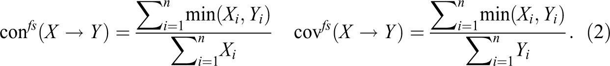
Since CCM-processed data $\text{δ}$ tend to feature various deficiencies (e.g., fragmentation, noise, etc.), expressions of type $\Phi \leftrightarrow Y$ that adhere to the strict standards of the equivalence operation (“ $\leftrightarrow$ ”) often cannot be inferred from $\text{δ}$ . To relax these standards, that is, to approximate strict sufficiency and necessity relations, Ragin (2006) introduced the consistency and coverage measures into the QCA protocol, which have subsequently also been imported into CNA (Baumgartner and Ambühl 2020). As the implication operator is defined differently in classical and in fuzzy logic, the two measures are defined differently for crisp-set and multi-value data, which both have a classical footing, and for fuzzy-set data. Cs-consistency ( ${\text{con}}^{cs}$ ) and cs-coverage ( ${\text{cov}}^{cs}$ ) of $X\to Y$ are defined as follows, where “ $|\dots {|}_{\text{δ}}$ ” represents the cardinality of the set of cases instantiating the enclosed expression in the data $\text{δ}$ :

${\text{con}}^{cs}(X\to Y)=\frac{{\left|X\ast Y\right|}_{\text{δ}}}{{\left|X\right|}_{\text{δ}}}\hspace{1em}\hspace{1em}{\text{cov}}^{cs}(X\to Y)=\frac{{\left|X\ast Y\right|}_{\text{δ}}}{{\left|Y\right|}_{\text{δ}}}.$

1

Fs-consistency ( ${\text{con}}^{fs}$ ) and fs-coverage ( ${\text{cov}}^{fs}$ ) of $X\to Y$ are defined as follows, where n is the number of cases in $\text{δ}$ :

${\text{con}}^{fs}(X\to Y)=\frac{{\displaystyle {\sum }_{i=1}^n}\text{min}(X_i,Y_i)}{{\displaystyle {\sum }_{i=1}^n}{X}_i}\hspace{1em}{\text{cov}}^{fs}(X\to Y)=\frac{{\displaystyle {\sum }_{i=1}^n}\text{min}(X_i,Y_i)}{{\displaystyle {\sum }_{i=1}^n}{Y}_i}.$

2

Whenever the values of X and Y are restricted to 1 and 0 in the crisp-set measures, ${\text{con}}^{cs}$ and ${\text{cov}}^{cs}$ coincide with ${\text{con}}^{fs}$ and ${\text{cov}}^{fs}$ , but for binary factors with values other than 1 and 0 and for multi-value factors that does not hold. Nonetheless, we will not explicitly distinguish between the cs and fs measures in the following because our discussion will make it sufficiently clear which of them is at issue.

What counts as acceptable scores on these measures is defined in threshold settings chosen by the analyst prior to the application of QCA or CNA. While QCA only accepts a consistency threshold, CNA requires both a consistency and a coverage threshold. Moreover, the implementation of these thresholds differs in important ways in the two methods. In QCA, a consistency threshold is imposed only on conjunctions of all exogenous factors (the so-called minterms) in the course of the generation of truth tables, which are intermediate calculative devices for QCA. The final models issued may or may not meet the chosen threshold. In CNA, thresholds for both consistency and coverage are used as authoritative model building constraints. The thresholds define what counts as sufficient and necessary conditions, to the effect that models not meeting them cannot be built.

Despite these differences, in both QCA and CNA, models with higher consistency and coverage are preferred over models with lower scores on these measures, provided they fare equally well in other respects (e.g., robustness). The following section introduces our procedure, ConCovOpt, calculating consistency and coverage optima.

The Optimization Procedure

The goal of ConCovOpt is to identify both optimal and maximal consistency and coverage scores—con-cov optima and con-cov maxima, for short—the distinction being that an optimum optimizes at least one of consistency and coverage, whereas a maximum optimizes their aggregate. The procedure is given configurational data $\text{δ}$ and a set of outcomes $O$ in $\text{δ}$ as an input. By suitably synthesizing $\text{δ}$ for the modeling of every $Y\in O$ , ConCovOpt first identifies output values for Boolean functions, so-called rep-assignments, which reproduce the behavior of Y as closely as possible, and, by calculating consistency and coverage scores for these rep-assignments, it then infers all con-cov optima and maxima that CCM models of Y can possibly reach.

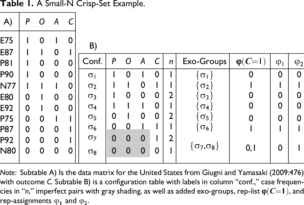
We introduce the procedure using the very simple $cs$ data example in Table 1A drawn from Giugni and Yamasaki (2009:476), who investigate the policy impact of different social movements between 1975 and 1995. The exogenous factors are high protest activity (P), public opinion favorable to the movement (O), and powerful institutional allies (A), with values 0 and 1 representing “no” and “yes” for all factors. The endogenous factor C takes the value 1 whenever a movement manages to significantly change a country’s policy and 0 otherwise. The authors analyze the data for various western countries separately; Table 1A features the data for the United States.

Table 1.

A Small-N Crisp-Set Example.

A)	P	O	A	C
E75	1	0	1	0
E87	1	1	0	1	B)
P81	1	0	0	0	Conf.	P	O	A	C	n	Exo-Groups	$\phi (C$ = $1)$	${\text{φ}}_1$	${\text{φ}}_2$
P90	1	0	0	0	${\text{σ}}_1$	1	0	1	0	1	$\left\{{\text{σ}}_1\right\}$	0	0	0
N77	1	1	1	0	${\text{σ}}_2$	1	1	0	1	1	$\left\{{\text{σ}}_2\right\}$	1	1	1
E80	0	1	0	0	${\text{σ}}_3$	1	0	0	0	2	$\left\{{\text{σ}}_3\right\}$	0	0	0
E92	0	1	0	0	${\text{σ}}_4$	1	1	1	0	1	$\left\{{\text{σ}}_4\right\}$	0	0	0
P75	0	0	1	1	${\text{σ}}_5$	0	1	0	0	2	$\left\{{\text{σ}}_5\right\}$	0	0	0
P87	0	0	0	1	${\text{σ}}_6$	0	0	1	1	1	$\left\{{\text{σ}}_6\right\}$	1	1	1
P92	0	0	0	1	${\text{σ}}_7$	0	0	0	1	2	$\{{\text{σ}}_7$ , ${\text{σ}}_8\}$	0,1	0	1
N80	0	0	0	0	${\text{σ}}_8$	0	0	0	0	1

Note: Subtable A) Is the data matrix for the United States from Giugni and Yamasaki (2009:476) with outcome C. Subtable B) is a configuration table with labels in column “conf.,” case frequencies in “n,” imperfect pairs with gray shading, as well as added exo-groups, rep-list $\phi (C$ = $1)$ , and rep-assignments ${\text{φ}}_1$ and ${\text{φ}}_2$ .

We begin by searching for con-cov optima for outcome C (i.e., C=1) in Table 1A. The notion of a con-cov optimum shall be defined as follows:

Con-Cov Optimum. An ordered pair $〈\text{con,cov}〉$ of consistency and coverage scores is a con-cov optimum for outcome Y= $\nu$ in data $\text{δ}$ iff, prior to applying a CCM, it can be excluded that a model of Y= $\nu$ inferred from $\text{δ}$ scores better on one element of the pair and at least as well on the other, whereas it cannot be excluded that a model of Y= $\nu$ reaches $〈\text{con,cov}〉$ .

If models of Y (i.e., Y=1) inferred from data $\text{δ}$ can be modeled with perfect consistency and coverage, $〈1,1〉$ is the only con-cov optimum for Y in $\text{δ}$ . Outcome C in Table 1A, however, does not have a con-cov optimum of $〈1,1〉$ . The reason is that the cases P87, P92, and N80 feature the same configuration of the exogenous factors—the configuration p $\ast$ o $\ast$ a—while C is given in P87 and P92 and c is given in N80. The configurations p $\ast$ o $\ast$ a $\ast$ C and p $\ast$ o $\ast$ a $\ast$ c constitute imperfect configurations, or what we will call an imperfect pair. ²

Imperfect Pair. An imperfect pair for Y= $\nu$ in data $\text{δ}$ is a pair of configurations $\{{\text{σ}}_i,{\text{σ}}_j\}$ in $\text{δ}$ , such that Y= $\nu$ is instantiated in one element of the pair and $Y\ne v$ in the other, while all other factors in $\text{δ}$ take constant values in both ${\text{σ}}_i$ and ${\text{σ}}_j$ .

In $cs$ (and $mv$ ) data $\text{δ}$ , there is a tight logical connection between imperfect pairs for an outcome Y and $〈1,1〉$ being the con-cov optimum for Y in $\text{δ}$ : Y has a con-cov optimum of $〈1,1〉$ in $\text{δ}$ iff there does not exist an imperfect pair for Y in $\text{δ}$ . The reason is that a model with perfect consistency and coverage expresses Y as a strict Boolean function of the other factors in $\text{δ}$ , and such a function issues exactly one output for every input. If there does not exist an imperfect pair for Y, every input (i.e., every configuration of factors other than Y) can be straightforwardly mapped either onto Y or onto y. But if there exists an imperfect pair, there exists an input to which no determinate output can be assigned, meaning Y cannot be expressed as a strict Boolean function of the other factors in $\text{δ}$ . On average, the more imperfect pairs Y has in $\text{δ}$ , the lower the con-cov optima for Y in $\text{δ}$ . ³

The existence of imperfect pairs indicates that there are varying causes of Y in the uncontrolled causal background. The variation of Y in an imperfect pair must have some cause or other but that cause cannot be among the other factors in $\text{δ}$ because they are constant in the pair. Since varying latent causes are a source of confounding, it is standardly recommended to try to resolve imperfect pairs prior to a CCM analysis; and there are various approaches on offer for how to do this (e.g., Rihoux and De Meur 2009). Of course, as suppressing the variation of latent causes, especially in observational studies, is very difficult, these approaches may be incapable of improving the data quality. For the purposes of this article, we will hence assume that the quality of all our example data has been improved as far as possible, meaning that the remaining imperfect pairs cannot be resolved.

A first step towards determining con-cov optima for an outcome Y is to identify imperfect pairs for Y in $\text{δ}$ . To do this in a methodical manner, we re-organize the data such that the instantiated configurations are rendered more transparent by synthesizing all cases in $\text{δ}$ instantiating the same configuration in a single row of what we call a configuration table. A configuration table $\text{CT}$ of data $\text{δ}$ merges multiple rows of $\text{δ}$ in which all factors have identical values into one row, such that each row of $\text{CT}$ corresponds to one determinate configuration of the factors in $\text{δ}$ . ⁴ The configurations in $\text{CT}$ are labeled and the number of cases instantiating each configuration is stored in a frequency column. The first three (line-separated) columns of Table 1B amount to a configuration table of the data in Table 1A.

A configuration table then allows for splitting the configurations into groups in which all factors other than a scrutinized outcome Y, that is, all factors exogenous with respect to Y, take constant values. We shall speak of exo-groups, for short.

Exo-Group. An exo-group of an outcome Y= $\nu$ in a configuration table $\text{CT}$ is a group of configurations in $\text{CT}$ with constant values in all factors in $\text{CT}$ other than Y.

The imperfect pairs for Y (i.e., Y=1) in data $\text{δ}$ can then be directly read off the list of Y’s exo-groups: Exo-groups with more than one element such that Y is instantiated in one element and not instantiated in another element correspond to imperfect pairs. To illustrate with our example, the exo-groups of C are listed in the fourth (line-separated) column of Table 1B. While ${\text{σ}}_1$ is the only configuration in Table 1B featuring P $\ast$ o $\ast$ A, meaning that $\left\{{\text{σ}}_1\right\}$ is a singleton exo-group of C, there are two configurations featuring p $\ast$ o $\ast$ a, namely, ${\text{σ}}_7$ and ${\text{σ}}_8$ , which constitute an exo-group with two elements $\{{\text{σ}}_7,{\text{σ}}_8\}$ . As C is instantiated in one element of that group and c in the other, $\{{\text{σ}}_7,{\text{σ}}_8\}$ amounts to an imperfect pair for C; and as C has no other exo-groups with more than one element, it is C’s only imperfect pair.

In order for a CCM model, which, to recall, has the form $\Phi \leftrightarrow Y$ , to have highest possible consistency and coverage, its redundancy-free DNF $\Phi$ must reproduce the instantiation behavior of the outcome Y as closely as possible. The notion of reproducing the behavior of an outcome as closely as possible will be of crucial importance for ConCovOpt. It must be understood somewhat differently for $cs$ and $mv$ data, on the one hand, and $fs$ data, on the other. In case of $cs$ and $mv$ data, we say that $\Phi$ reproduces the behavior of an outcome as closely as possible iff $\Phi$ returns the value 1 for every exo-group in which the outcome is constantly instantiated, 0 for every exo-group in which it is constantly non-instantiated, and either 0 or 1 for every exo-group with a varying instantiation of the outcome. Applied to our example, this means that a $\Phi$ —whichever concrete DNF this may be—reproduces the behavior of C as closely as possible iff $\Phi$ returns 1 for exo-groups $\left\{{\text{σ}}_2\right\}$ and $\left\{{\text{σ}}_6\right\}$ ; 0 for $\left\{{\text{σ}}_1\right\}$ , $\left\{{\text{σ}}_3\right\}$ , $\left\{{\text{σ}}_4\right\}$ , and $\left\{{\text{σ}}_5\right\}$ ; and either 0 or 1 for ${\text{{σ}}_{\text{7}}{\text{,σ}}_{\text{8}}\text{}}$ . Taken together, these value assignments yield what we will call the rep-list (reproduction list) $\phi (C$ = $1)$ for outcome C in Table 1B.

Rep-List. A rep-list $\phi (Y$ = $\nu )$ for an outcome Y= $\nu$ assigns all the values reproducing the behavior of Y= $\nu$ as closely as possible to every exo-group of Y= $\nu$ .

Moreover, to an assignment that returns a value from a rep-list for every exo-group, we will refer as a rep-assignment (reproduction assignment).

Rep-Assignment. A rep-assignment $\text{φ}$ for an outcome Y= $\nu$ assigns exactly one value from a rep-list $\phi (Y$ = $\nu )$ to every exo-group of Y= $\nu$ .

Whatever concrete factor values CCMs may ultimately incorporate in DNFs accounting for outcome Y, it is clear—prior to applications of CCMs—that a DNF not returning a rep-assignment does not reach a con-cov optimum for Y. At the same time, as will be shown in the next section, some rep-assignments yield non-optimal consistency or coverage scores. That is, returning a rep-assignment for Y is necessary but not sufficient for a DNF to reach a con-cov optimum for Y. In order to identify those rep-assignments that actually yield con-cov optima, all possible rep-assignments must be built from $\phi (Y$ = $\nu )$ and the consistency and coverage scores they induce tested for optimality.

The number of rep-assignments that can be built from a rep-list $\phi (Y$ = $\nu )$ is equal to the number of combinatorially possible value distributions drawn from $\phi (Y$ = $\nu )$ , that is, to ${\displaystyle {\prod }_{i=1}^n}|\phi (Y$ = $\nu {)}_i|$ , where n is the number of exo-groups and $|\phi (Y$ = $\nu {)}_i|$ the cardinality of the set of possible values assigned to exo-group i. In our example, the complete set of rep-assignments is easily built, as there is only one exo-group with more than one value in the rep-list $\phi (C\mathbf{=}1)$ . Hence, outcome C has a total of two rep-assignments, ${\text{φ}}_1$ and ${\text{φ}}_{\text{2}}$ , which are featured in the last two columns of Table 1B. ${\text{φ}}_{\text{1}}$ and ${\text{φ}}_{\text{2}}$ coincide except for the fact that they contain the values 0 and 1, respectively, for exo-group $\{{\text{σ}}_7,{\text{σ}}_8\}$ . ${\text{φ}}_{\text{1}}$ induces perfect consistency but does not cover the instance of C in ${\text{σ}}_{\text{7}}$ , whereas ${\text{φ}}_{\text{2}}$ covers the instance of C in ${\text{σ}}_{\text{7}}$ but violates perfect consistency in ${\text{σ}}_{\text{8}}$ .

It only remains to be determined which of all rep-assignments actually reach con-cov optima. To this end, consistency and coverage scores are calculated for all rep-assignments. In case of $cs$ and $mv$ data, this can be done by plugging the values of a rep-assignment ${\text{φ}}_i$ and the corresponding instantiation behavior of outcome Y= $\nu$ into the definitions ${\text{con}}^{cs}$ and ${\text{cov}}^{cs}$ in expression (1). In our example, this means that columns “ ${\text{φ}}_{\text{1}}$ ” and “ ${\text{φ}}_{\text{2}}$ ” of Table 1B yield the X-values of ${\text{con}}^{cs}$ and ${\text{cov}}^{cs}$ , column “C” the Y-values, and column “n” the case frequencies. We get the following consistency and coverage scores:

${\text{φ}}_1:\hspace{1em}\text{con}=1;\hspace{1em}\text{cov}=0.5,$

3

${\text{φ}}_2:\hspace{1em}\text{con}=0.8;\hspace{1em}\text{cov}=1.$

4

Due to the imperfect pair in exo-group ${\text{{σ}}_{\text{7}}{\text{,σ}}_{\text{8}}\text{}}$ , it is impossible, in principle, for a CCM model of C inferred from the data in Table 1A to score better on consistency and coverage. ${\text{φ}}_{\text{1}}$ outperforms ${\text{φ}}_{\text{2}}$ in consistency and ${\text{φ}}_{\text{2}}$ outperforms ${\text{φ}}_{\text{1}}$ in coverage. As neither of the two scores better than the other on one measure and at least as well on the other, they are both con-cov optima. ${\text{φ}}_{\text{1}}$ optimizes consistency, and ${\text{φ}}_{\text{2}}$ optimizes coverage. At the same time, ${\text{φ}}_{\text{2}}$ clearly outperforms ${\text{φ}}_{\text{1}}$ in the aggregate of consistency and coverage, which we take to be the product of consistency and coverage (i.e., the con-cov product). That is, ${\text{φ}}_{\text{2}}$ has the better overall model fit; it reaches a con-cov maximum:

Con-Cov Maximum. An ordered pair $〈\text{con, cov}〉$ of consistency and coverage scores is a con-cov maximum for outcome Y= $\nu$ in data $\text{δ}$ iff $〈\text{con, cov}〉$ is a con-cov optimum for Y = $\nu$ in $\text{δ}$ with the highest aggregate, that is, product, of consistency and coverage.

Of course, the product of consistency and coverage is only one option among many to aggregate consistency and coverage. Assessing the overall model fit based on the con-cov product amounts to giving equal weights to consistency and coverage, which, while standard in CNA, may not be endorsed by all QCA methodologists (who tend to have a preference for consistency). We do not want to take a stance on that issue here but, instead, invite a reader who wants to assess the overall model fit by giving unequal weights to consistency and coverage to view the simple con-cov product in the above definition as a placeholder for any preferred function aggregating consistency and coverage. That is, a con-cov maximum might alternatively be defined as a con-cov optimum with maximal score on ${\text{con}}^{0.75}\cdot {\text{cov}}^{0.25}$ , or on $(0.25\cdot \text{con})+(0.75\cdot \text{cov})$ , or on $\text{min(con, cov)}$ , and so on. ⁵ While all of these alternative definitions identify ${\text{φ}}_{\text{2}}$ as con-cov maximum for outcome C, they may select different con-cov maxima in other examples. Still, to avoid unnecessary complications, we shall subsequently only work with the con-cov product as our aggregation function of choice.

In sum, without having applied CCMs to Guigni and Yamasaki’s (2009) data, we have identified optimal and maximal consistency and coverage scores for them. Before we search for actual CCM models for our example, let us assemble the different procedural steps. To this end, one generalization is still needed. For simplicity, all data analyzed in this article comprise a single outcome only, but, of course, configurational data may feature multiple outcomes. If that is the case, exo-groups, rep-lists, and rep-assignments must be formed and consistency and coverage scores calculated for each outcome separately. For generality, we thus let the input of ConCovOpt be data $\text{δ}$ along with a set of outcomes $O$ in $\text{δ}$ . If no prior knowledge is available as to which values of which factors in $\text{δ}$ are possible outcomes, ConCovOpt can simply be run by setting $O$ equal to all values of all factors in $\text{δ}$ . ConCovOpt is presented in Procedure 1.

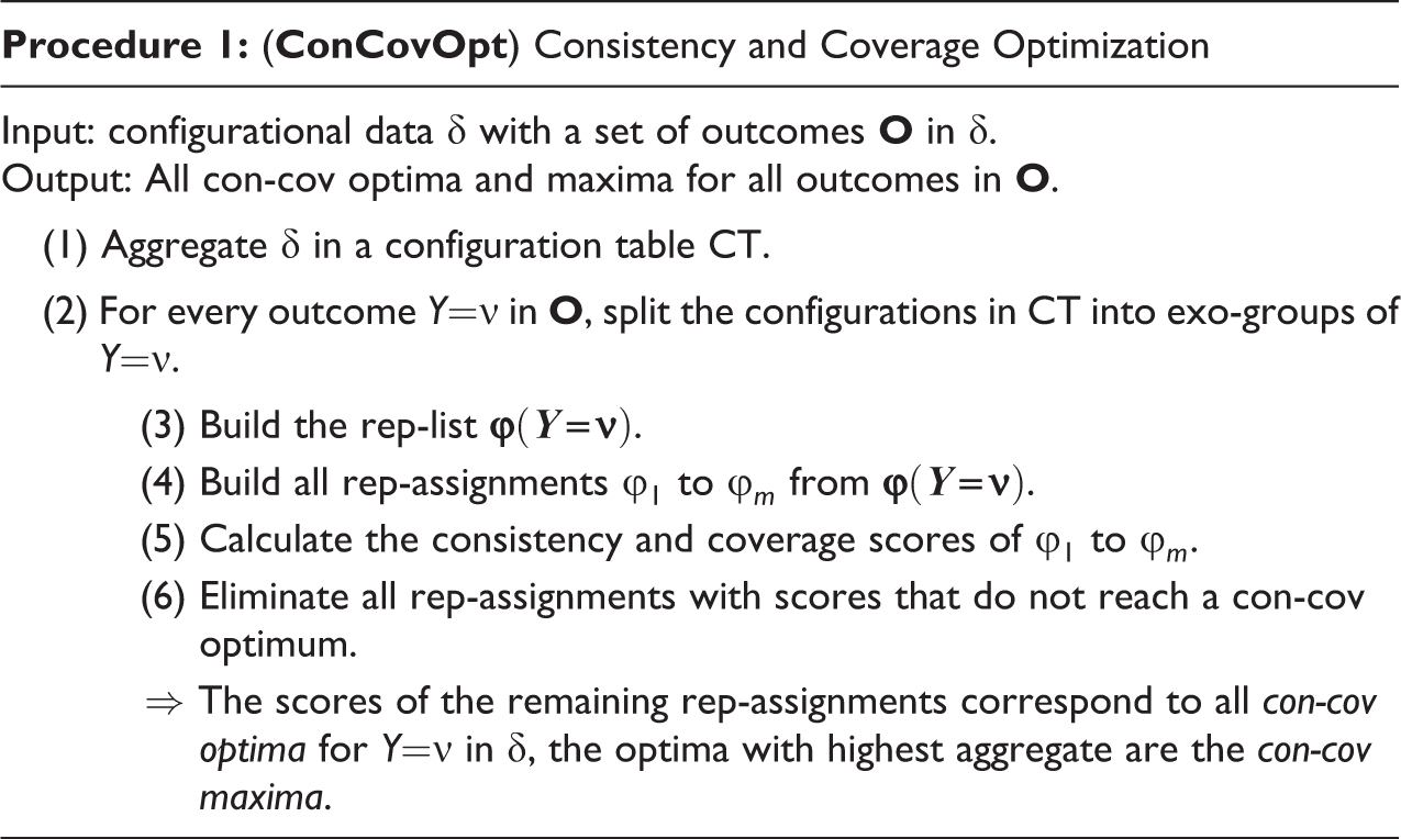
Procedure 1: (ConCovOpt) Consistency and Coverage Optimization

Input: configurational data $\text{δ}$ with a set of outcomes $O$ in $\text{δ}$ .Output: All con-cov optima and maxima for all outcomes in $O$ .(1) Aggregate $\text{δ}$ in a configuration table $\text{CT}$ .(2) For every outcome Y= $\nu$ in $O$ , split the configurations in $\text{CT}$ into exo-groups of Y= $\nu$ . (3) Build the rep-list $\phi (Y$ = $\nu )$ . (4) Build all rep-assignments ${\text{φ}}_{\text{1}}$ to ${\text{φ}}_m$ from $\phi (Y$ = $\nu )$ . (5) Calculate the consistency and coverage scores of ${\text{φ}}_{\text{1}}$ to ${\text{φ}}_m$ . (6) Eliminate all rep-assignments with scores that do not reach a con-cov optimum.⇒ The scores of the remaining rep-assignments correspond to all con-cov optima for Y= $\nu$ in $\text{δ}$ , the optima with highest aggregate are the con-cov maxima.

Let us now apply CCMs to our example data in order to find actual models returning ${\text{φ}}_{\text{1}}$ and ${\text{φ}}_{\text{2}}$ . At a consistency threshold anywhere between 1 and $0.67$ , QCA produces the following parsimonious (QCA-PS) and conservative models (QCA-CS), ⁶ the latter of which is also the model published by Giugni and Yamasaki (2009:479):

$\text{QCA}-\text{PS:}\hspace{1em}p\ast A+P\ast O\ast a\leftrightarrow C\hspace{1em}\hspace{1em}\text{con}=1;\text{cov}=0.5,$

5

$\text{QCA}-\text{CS:}\hspace{1em}p\ast o\ast A+P\ast O\ast a\leftrightarrow C\hspace{1em}\hspace{1em}\text{con}=1;\text{cov}=\mathrm{0.5.}$

6

In both equations (5) and (6), not only the solution consistency but also the consistencies of all sufficient conditions (i.e., disjuncts) are 1. Our previous calculations attest that the QCA models reach a con-cov optimum, as they return rep-assignment ${\text{φ}}_{\text{1}}$ . At the same time, we now see that equations (5) and (6) do not reach a con-cov maximum. Rep-assignment ${\text{φ}}_{\text{2}}$ shows that it is possible to significantly improve on the overall model fit. But at a conventional consistency threshold of 0.75, standard QCA does not find a better scoring model—for two main reasons. On the one hand, QCA builds models from the top down by first searching for complete minterms satisfying a chosen consistency threshold and then eliminating redundancies. The minterm p $\ast$ o $\ast$ a of the exo-group ${\text{{σ}}_{\text{7}}{\text{,σ}}_{\text{8}}\text{}}$ , however, only reaches a consistency of $0.667$ and is therefore not further considered by QCA (in QCA jargon: it is coded “0”)—despite the fact that, as we shall see below, a proper part of that minterm indeed scores $0.75$ on consistency. On the other hand, standard QCA does not accept a coverage threshold and, hence, cannot be “asked” to build models with specific target scores on coverage.

CNA, by contrast, accepts separate thresholds for consistency of sufficient conditions and of whole models as well as for coverage of whole models. It can thus be “asked” to build models at any target scores. Moreover, it builds models from the bottom up by first testing single factor values for compliance with chosen thresholds and by then gradually adding further factor values until threshold compliance is established. ⁷ Dusa (2018) has recently presented a promising new algorithm for QCA called CCubes that also builds models from the bottom up and accepts the same types of thresholds as CNA. ⁸ At a threshold setting of $〈1,0.5〉$ , CNA and CCubes return the same model as QCA-PS, but at $〈0.75,1〉$ , they find the following model realizing ${\text{φ}}_{\text{2}}$ :

$\text{CNA/CCubes:}\hspace{1em}p\ast o+P\ast O\ast a\leftrightarrow C\hspace{1em}\hspace{1em}\text{con}=0.8;\text{\hspace{1em}cov}=1.$

7

This is not the place to select among the different model candidates we have now recovered for Guigni and Yamasaki’s (2009) data, nor to substantively interpret them. What matters for our purposes is that computing con-cov optima and maxima by means of ConCovOpt prior to actually conducting CCM analyses has (at least) three important payoffs. First, it allows us to determine how close actually obtained models come to optimal and maximal fit. Second, it renders transparent whether the obtained models exhaust the space of con-cov optima or whether further models should be searched at different thresholds. Third, without having to try out a whole range of threshold settings, CCMs can be run by directly constraining them towards optimal thresholds.

Large-N Crisp-set Data

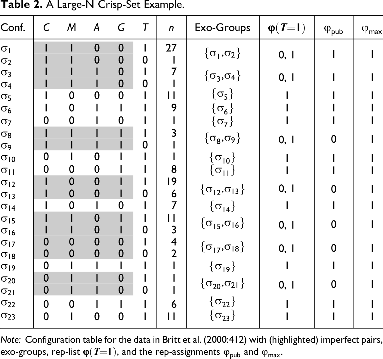
The data in Table 1A are very simple and, although the resulting optimal models differ significantly in overall fit, they have a considerable overlap in causal ascriptions, thus inducing only marginally different causal conclusions. To show that optimizing consistency and coverage can also make a substantive difference in causal conclusions, we now turn to a more intricate, large-N data example. Britt et al. (2000) investigate the determinants leading to the parental decision to terminate a pregnancy after a prenatal diagnosis of trisomy 21. Four exogenous factors are examined: existing children (C; 0 $:=$ “none,” 1 $:=$ “1 or more”), maternal age in years (M; 0 $:=$ “37 and under,” 1 $:=$ “38 and above”), prior voluntary abortions (A; 0 $:=$ “none,” 1 $:=$ “1 or more”), and gestational age in weeks (G; 0 $:=$ “16 and under,” 1 $:=$ “17 and over”). The endogenous factor is termination (T; $0:=$ “continue,” 1 $:=$ “terminate”). The cases are 142 pregnant women receiving a trisomy 21 diagnosis at Wayne State University Clinic from September 1989 through October 1998. The complete data can be consulted in our replication script, and the configuration table resulting from that data is given in Table 2.

Table 2.

A Large-N Crisp-Set Example.

Conf.	C	M	A	G	T	n	Exo-Groups	$\phi (T$ = $1)$	${\phi }_{\text{pub}}$	${\phi }_{\text{max}}$
${\text{σ}}_{\text{1}}$	1	1	0	0	1	27	${\text{{σ}}_{\text{1}}$ , ${\text{σ}}_{\text{2}}\text{}}$	0, 1	1	1
${\text{σ}}_{\text{2}}$	1	1	0	0	0	1
${\text{σ}}_{\text{3}}$	1	1	1	0	1	7	${\text{{σ}}_{\text{3}}$ , ${\text{σ}}_{\text{4}}\text{}}$	0, 1	1	1
${\text{σ}}_{\text{4}}$	1	1	1	0	0	1
${\text{σ}}_{\text{5}}$	1	0	0	0	1	11	${\text{{σ}}_{\text{5}}\text{}}$	1	1	1
${\text{σ}}_{\text{6}}$	1	0	1	1	1	9	${\text{{σ}}_{\text{6}}\text{}}$	1	1	1
${\text{σ}}_{\text{7}}$	0	0	1	0	1	1	${\text{{σ}}_{\text{7}}\text{}}$	1	1	1
${\text{σ}}_{\text{8}}$	1	1	1	1	1	3	${\text{{σ}}_{\text{8}}$ , ${\text{σ}}_{\text{9}}\text{}}$	0, 1	0	1
${\text{σ}}_{\text{9}}$	1	1	1	1	0	1
${\text{σ}}_{\text{10}}$	0	1	0	1	1	1	${\text{{σ}}_{\text{10}}\text{}}$	1	1	1
${\text{σ}}_{\text{11}}$	0	0	0	1	1	8	${\text{{σ}}_{\text{11}}\text{}}$	1	1	1
${\text{σ}}_{\text{12}}$	1	0	0	1	1	19	${\text{{σ}}_{\text{12}}$ , ${\text{σ}}_{\text{13}}\text{}}$	0, 1	0	1
${\text{σ}}_{\text{13}}$	1	0	0	1	0	6
${\text{σ}}_{\text{14}}$	1	0	1	0	1	7	${\text{{σ}}_{\text{14}}\text{}}$	1	1	1
${\text{σ}}_{\text{15}}$	1	1	0	1	1	11	${\text{{σ}}_{\text{15}}$ , ${\text{σ}}_{\text{16}}\text{}}$	0, 1	0	1
${\text{σ}}_{\text{16}}$	1	1	0	1	0	3
${\text{σ}}_{\text{17}}$	0	0	0	0	1	4	${\text{{σ}}_{\text{17}}$ , ${\text{σ}}_{\text{18}}\text{}}$	0, 1	0	1
${\text{σ}}_{\text{18}}$	0	0	0	0	0	2
${\text{σ}}_{\text{19}}$	0	1	1	1	1	1	${\text{{σ}}_{\text{19}}\text{}}$	1	1	1
${\text{σ}}_{\text{20}}$	0	1	1	0	1	1	${\text{{σ}}_{\text{20}}$ , ${\text{σ}}_{\text{21}}\text{}}$	0, 1	0	1
${\text{σ}}_{\text{21}}$	0	1	1	0	0	1
${\text{σ}}_{\text{22}}$	0	0	1	1	1	6	${\text{{σ}}_{\text{22}}\text{}}$	1	1	1
${\text{σ}}_{\text{23}}$	0	1	0	0	1	11	${\text{{σ}}_{\text{23}}\text{}}$	1	1	1

Note: Configuration table for the data in Britt et al. (2000:412) with (highlighted) imperfect pairs, exo-groups, rep-list $\phi (T$ = $1)$ , and the rep-assignments ${\text{φ}}_{\text{pub}}$ and ${\text{φ}}_{\text{max}}$ .

As is frequently the case in large-N data, there are numerous imperfect pairs, highlighted with gray shading. Instead of first calculating con-cov optima and maxima and only afterwards looking at concrete models, we proceed in reverse order for this example. We begin by presenting the model offered by Britt et al. (2000:412). They choose a consistency threshold of $0.875$ . At this threshold, QCA builds two models (only the second of which is mentioned by the authors): ⁹

$\text{QCA:}\hspace{1em}c\ast G+C\ast g+m\ast A+c\ast M\ast a\leftrightarrow T\hspace{1em}\hspace{1em}\text{con}=0.98;\text{cov}=0.70,$

8

$c\ast G+C\ast g+m\ast A+M\ast a\ast g\leftrightarrow T\hspace{1em}\hspace{1em}\text{con}=0.98;\text{cov}=\mathrm{0.70.}$

9

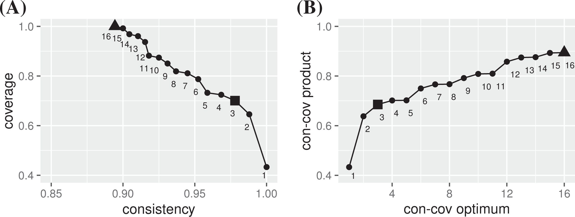
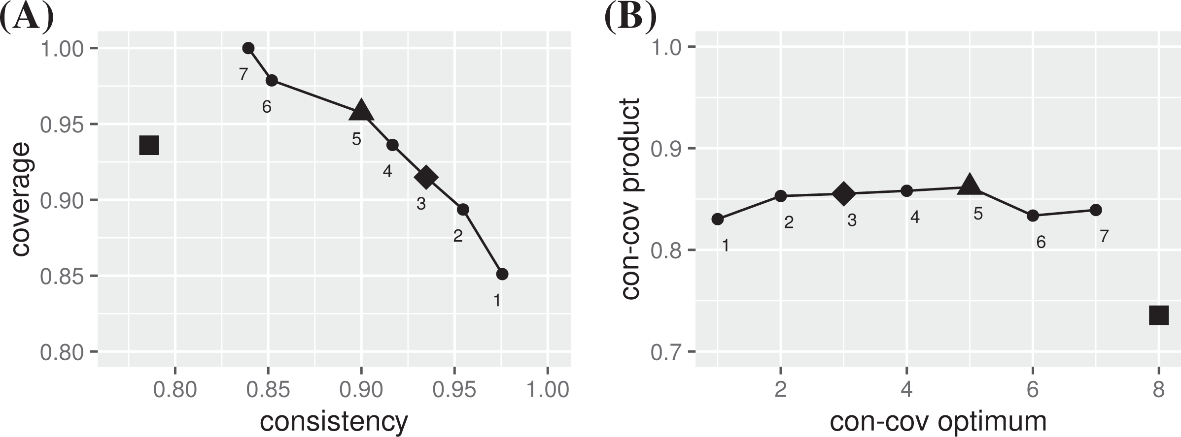
A handful of QCA re-runs with only slightly varied consistency thresholds show that the results are highly volatile, yielding many different models with different overall fit. Identifying a con-cov maximum for these data calls for a systematic approach. We thus apply ConCovOpt with $O=\{T=1\}$ . The result of step (1) is the configuration table in Table 2. Step (2) yields nine singleton exo-groups entailing determinate values for the rep-list in step (3). In all seven non-singleton exo-groups, the outcome T varies, meaning that DNFs reproducing the behavior of T as closely as possible can return either 0 or 1 for those groups. In total, the resulting rep-list $\phi (T\mathrm{=}1)$ induces $2^7=128$ rep-assignments in step (4). In step (5), consistency and coverage scores are calculated for all of them and those with non-optimal scores eliminated in step (6). Sixteen con-cov optima remain. They are plotted in Figure 1A.

Figure 1.

Plot A shows the 16 con-cov optima for outcome T in the data of Britt et al. (2000) and Plot B shows the con-cov products of each optimum. $▴$ is the con-cov maximum and $\blacksquare$ is the published model.

In light of these results, we can now say that the published model (9), which scores $〈0.98,0.70〉$ , indeed reaches a con-cov optimum ( ${\text{φ}}_{\text{3}}$ ; $\blacksquare$ in Figure 1). However, with its con-cov product of $0.69$ , it is quite far away from a con-cov maximum. The con-cov products of all 16 optima are plotted in Figure 1B. The con-cov maximum for outcome T is ${\text{φ}}_{\text{16}}$ $〈0.89,1〉$ ( $▴$ ). For transparency, we add the rep-assignment ${\text{φ}}_{pub}$ (i.e., ${\text{φ}}_3$ ) realized by the published model and the assignment ${\text{φ}}_{\text{max}}$ (i.e., ${\text{φ}}_{16}$ ) yielding the con-cov maximum to Table 2.

The value distribution of ${\text{φ}}_{\text{max}}$ is striking: It assigns 1 to every exo-group, resulting in a (vacuous) tautology. In other words, a best fitting model for the data of Britt et al. (2000) entails that pregnancy is terminated in case of a trisomy 21 diagnosis whatever the values of the exogenous factors, that is, independently of the pregnant woman’s existing children, prior abortions, age, and gestational age. To render this more concrete, let us now search for actual models at $〈0.89,1〉$ . While standard QCA algorithms do not find a model reaching the con-cov maximum, CNA and CCubes have no problem finding such a model. At a threshold setting of $〈0.89,1〉$ , the following tautologous model is returned: ¹⁰

$\text{CNA/CCubes:}\hspace{1em}M+m\leftrightarrow T\hspace{1em}\hspace{1em}\text{con}=0.89;\text{cov}=1.$

10

Of course, any other tautologous model, as $C+c\leftrightarrow T$ or $A+a\leftrightarrow T$ , reaches the same fit scores, but equation (10) is the only model such that the two disjuncts M and m individually reach the consistency threshold of $0.89$ as well—which is why it is the only model issued by CNA and CCubes. The overall fit of equation (10) is good by all CCM standards, and equation (10) also meets the consistency threshold used by Britt et al. (2000). It is the best fitting model for their data, and, for principled reasons, its fit scores cannot be outperformed. But of course, it is not a causally interpretable model. Causes are difference makers of their effects, yet a tautology does not make a difference to anything.

This finding casts doubts on all causal conclusions Britt et al. (2000) have drawn from their data; 127 of all 141 women receiving a trisomy 21 diagnosis in their sample choose to terminate, making termination the canonical response to the diagnosis. No non-tautologous function of the exogenous factors can account for the outcome better than the tautologous model that entails termination no matter what. The data contain too little variation on the outcome T to conclude anything about its causes; in particular, there is no evidence that T is caused by any of the factors C, M, A, or G. A causal interpretation of the published model (9) is unwarranted by the data. This shows that a systematic search for con-cov maxima (prior to a CCM analysis) may have implications that go way beyond minor model adjustments or improvements. The optimization of consistency and coverage scores rendered possible by ConCovOpt may thoroughly change the conclusions drawn from a study.

Multi-value Data

ConCovOpt is straightforwardly applicable to multi-value data. Although the factors in $mv$ data can take more than two values, models for an $mv$ outcome Y= $\nu$ have the same logical form as $cs$ models: They account for Y= $\nu$ in terms of redundancy-free DNFs, which, irrespective of whether they feature $cs$ or $mv$ factors, are true or false, that is, only return 1 or 0. Hence, for an optimal $mv$ DNF to reproduce the instantiation behavior of an outcome Y= $\nu$ as closely as possible, the exact same conditions must be satisfied as in the $cs$ case. It follows that rep-lists and rep-assignments can be built and evaluated for consistency and coverage in exactly the same way for $mv$ data as for $cs$ data.

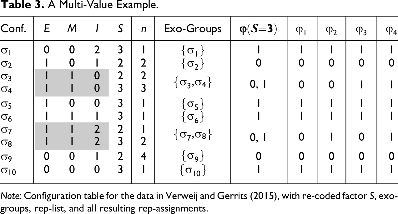
To illustrate, we apply ConCovOpt to the $mv$ data of Verweij and Gerrits (2015), who investigate the impact of different management strategies in response to unplanned events occurring during the implementation of a large infrastructure project in Maastricht. Their data comprise 18 unplanned events (between 2009 and 2011) measuring the following exogenous factors: nature of the event (E; 0 $:=$ “physical/remote,” 1 $:=$ “social/project/public”), nature of the management response (M; 0 $:=$ “internal,” 1 $:=$ “external”), and nature of the interaction between public and private managers (I; 0 $:=$ “autonomous public,” 1 $:=$ “autonomous private,” 2 $:=$ “cooperation”). The endogenous factor is the satisfactoriness of the management response (S). To emphasize the data’s $mv$ nature, we replace the original values of S (i.e., 0 and 1) by two (arbitrarily chosen) different ones; that is, we will say that S takes the value 3 if satisfactoriness is high and the value 2 if it is not high.

The input to ConCovOpt, hence, is Verweij and Gerrits’s complete data with $O=\{S=3\}$ (see the replication script). In step (1), ConCovOpt synthesizes that data in the configuration table contained in Table 3. As there is only one outcome, step (2) forms one set of exo-groups, which are listed in column 4. There are two non-singleton exo-groups, ${\text{{σ}}_{\text{3}}$ , ${\text{σ}}_{\text{4}}\text{}}$ and ${\text{{σ}}_{\text{7}}$ , ${\text{σ}}_{\text{8}}\text{}}$ , each inducing two possible values in the rep-list in step (3). Step (4) generates $2^2=4$ rep-assignments ${\text{φ}}_{\text{1}}$ to ${\text{φ}}_{\text{4}}$ . For transparency, we list them all in Table 3. In step (5), the value distributions of ${\text{φ}}_{\text{1}}$ to ${\text{φ}}_{\text{4}}$ and the instantiation behavior of outcome S=3 are plugged into ${\text{con}}^{cs}$ and ${\text{cov}}^{cs}$ . Step (6) checks the consistency and coverage scores for optimality, which check is positive for all scores. Overall, ConCovOpt identifies the following four con-cov optima for outcome S=3, the last of which, ${\text{φ}}_{\text{4}}$ , is a con-cov maximum:

${\text{φ}}_{\text{1}}:\hspace{1em}\text{con}=1;\hspace{1em}\text{cov}=0.44,$

11

${\text{φ}}_{\text{2}}:\hspace{1em}\text{con}=0.86;\hspace{1em}\text{cov}=0.67,$

12

${\text{φ}}_3:\hspace{1em}\text{con}=0.78;\hspace{1em}\text{cov}=0.78,$

13

${\text{φ}}_4:\hspace{1em}\text{con}=0.75;\hspace{1em}\text{cov}=1.$

14

Table 3.

A Multi-Value Example.

Conf.	E	M	I	S	n	Exo-Groups	$\phi (S$ = $3)$	${\text{φ}}_{\text{1}}$	${\text{φ}}_{\text{2}}$	${\text{φ}}_{\text{3}}$	${\text{φ}}_{\text{4}}$
${\text{σ}}_{\text{1}}$	0	0	2	3	1	${\text{{σ}}_{\text{1}}\text{}}$	1	1	1	1	1
${\text{σ}}_{\text{2}}$	1	0	1	2	2	${\text{{σ}}_{\text{2}}\text{}}$	0	0	0	0	0
${\text{σ}}_{\text{3}}$	1	1	0	2	2	${\text{{σ}}_{\text{3}}$ , ${\text{σ}}_{\text{4}}\text{}}$	0, 1	0	0	1	1
${\text{σ}}_{\text{4}}$	1	1	0	3	3
${\text{σ}}_{\text{5}}$	1	0	0	3	1	${\text{{σ}}_{\text{5}}\text{}}$	1	1	1	1	1
${\text{σ}}_{\text{6}}$	1	1	1	3	1	${\text{{σ}}_{\text{6}}\text{}}$	1	1	1	1	1
${\text{σ}}_{\text{7}}$	1	1	2	2	1	${\text{{σ}}_{\text{7}}$ , ${\text{σ}}_{\text{8}}\text{}}$	0, 1	0	1	0	1
${\text{σ}}_{\text{8}}$	1	1	2	3	2
${\text{σ}}_{\text{9}}$	0	0	1	2	4	${\text{{σ}}_{\text{9}}\text{}}$	0	0	0	0	0
${\text{σ}}_{\text{10}}$	0	0	0	3	1	${\text{{σ}}_{\text{10}}\text{}}$	1	1	1	1	1

Note: Configuration table for the data in Verweij and Gerrits (2015), with re-coded factor S, exo-groups, rep-list, and all resulting rep-assignments.

Verweij and Gerrits (2015:21) present a conservative solution, equation (15), that scores $〈1,0.44〉$ and, hence, realizes the optimum ${\text{φ}}_{\text{1}}$ . Independently of where in the interval $[1,0.67]$ the consistency threshold is placed, QCA finds two parsimonious solutions, equations (16) and (17), which likewise realize ${\text{φ}}_{\text{1}}$ .

$\text{QCA}-\text{CS:}\hspace{1em}M\text{=}0\ast I\text{=}0+E\text{=}0\ast M\text{=}0\ast I\text{=}2+E\text{=}1\ast M\text{=}1\ast I\text{=}1\leftrightarrow S\text{=}3,$

15

$\text{QCA}-\text{PS:}\hspace{1em}M\text{=}0\ast I\text{=}0+E\text{=}0\ast I\text{=}2+M\text{=}1\ast I\text{=}1\leftrightarrow S\text{=}3,$

16

$M\text{=}0\ast I\text{=}0+M\text{=}0\ast I\text{=}2+M\text{=}1\ast I\text{=}1\leftrightarrow S\text{=}3.$

17

That is, in the range of conventional threshold settings, QCA only finds models realizing one of the four con-cov optima. Instead of now applying CNA and CCubes, we next introduce a procedure for building CCM models realizing any con-cov optimum for $cs$ and $mv$ data.

A con-cov optimum is realized by a DNF that outputs either 1 or 0 for every exo-group. Any two DNFs that return the same output for all exo-groups have the same consistency and coverage. For convenience, let us call the set of exo-groups to which a rep-assignment ${\text{φ}}_i$ assigns the value 1 the positive group of ${\text{φ}}_i$ . One particularly interesting DNF returning ${\text{φ}}_i$ then is what we label ${\text{φ}}_i$ ’s canonical DNF—in reference to canonical normal forms of logical expressions (Lemmon 1965:198).

Canonical DNF. The canonical DNF returning a rep-assignment ${\text{φ}}_i$ for outcome Y= $\nu$ is the disjunction of the configurations of all factors exogenous to Y in ${\text{φ}}_i$ ’s positive group.

Just as any logical expression is guaranteed to have a unique canonical normal form, so is every rep-assignment guaranteed to have exactly one canonical DNF, which moreover is easily built. For example, disjunctively concatenating the configurations of factors E, M, and I in ${\text{φ}}_4$ ’s positive group in Table 3 yields the canonical DNF returning ${\text{φ}}_4$ ; it is a DNF that scores $〈0.75,1〉$ in accounting for S=3:

$E\text{=}0\ast M\text{=}0\ast I\text{=}2+E\text{=}1*M\text{=}1\ast I\text{=}0+E\text{=}1\ast M\text{=}0\ast I\text{=}0+E\text{=}1\ast M\text{=}1\ast I\text{=}1+E\text{=}1\ast M\text{=}1\ast I\text{=}2+E\text{=}0\ast M\text{=}0\ast I\text{=}0.$

18In the same way, the canonical DNFs of the other con-cov optima for outcome S=3 can be construed. For example, as the exo-group ${\text{{σ}}_{\text{7}}{\text{,σ}}_{\text{8}}\text{}}$ is not in ${\text{φ}}_{\text{3}}$ ’s positive group, removing the configuration of the exogenous factors in ${\text{{σ}}_{\text{7}}{\text{,σ}}_{\text{8}}\text{}}$ , namely, E= $1\ast$ $M$ = $1\ast$ $I$ =2, from equation (18) is all it takes to build the canonical DNF returning ${\text{φ}}_{\text{3}}$ .

Of course, as canonical DNFs comprise all configurations of all exogenous factors in an optimum’s positive group, they tend not to be redundancy-free, and consequently, not to be causally interpretable. For instance, if we remove E=0 from the first and the last disjuncts in equation (18), we are still left with a DNF with the same output for all exo-groups in Table 3, that is, a DNF returning ${\text{φ}}_{\text{4}}$ . The same holds if we continue to eliminate E=1 from all disjuncts. By contrast, if I=2 is eliminated from the first disjunct of equation (18), we are left with a DNF that scores $〈0.56,1〉$ in accounting for S=3 and, thus, no longer returns ${\text{φ}}_{\text{4}}$ . The reason is that a DNF featuring E= $0\ast$ $M$ =0 as a separate disjunct (instead of E= $0$ $\ast M$ = $0\ast$ $I$ =2) outputs 1 for exo-group ${\text{{σ}}_{\text{9}}\text{}}$ , whereas ${\text{φ}}_{\text{4}}$ assigns 0 to that group. In sum, while some factor values can be removed from equation (18) such that the remaining DNF still returns ${\text{φ}}_{\text{4}}$ , others are indispensable for returning ${\text{φ}}_{\text{4}}$ .

These considerations suggest that equation (18) can be turned into a redundancy-free DNF returning ${\text{φ}}_{\text{4}}$ by systematically removing factor values and checking whether the remainder still outputs the same as equation (18) for all exo-groups. All factor values for which this check is positive are redundant; all factor values for which the check is negative are indispensable (non-redundant). If all redundancies are removed from equation (18), we are left with this redundancy-free DNF: I= $2+I$ = $0+M$ =1. Accounting for S=3 on its basis yields the following model, which reaches the con-cov maximum for Verweij and Gerrits’s data:

$I\text{=}2+I\text{=}0+M\text{=}1\leftrightarrow S\text{=}3\hspace{1em}\hspace{1em}\text{con}=0.75;\hspace{1em}\text{cov}=1.$

19

Model (19) has a peculiarity. Although the model as a whole reaches a consistency of $0.75$ , two of its component disjuncts do not. M=1 and I=0 are sufficient for S=3 with consistencies of $0.67$ and $0.71$ only. It follows that in order to find model (19) with CNA and CCubes, the consistency threshold must be lowered to $0.66$ . Whether models some of whose components only reach a consistency of $0.67$ should be considered acceptable is a question that requires further discussion, which, however, goes beyond the purposes of this article. If model (19) is considered unacceptable, our previous analysis has shown that there are other con-cov optima on offer for Verweij and Gerrits’s data that score better than the published model. For example, by systematically eliminating redundancies from the canonical DNF returning ${\text{φ}}_{\text{2}}$ , we find the redundancy-free DNF in equation (20), all of whose disjuncts have consistencies of $0.75$ or higher, such that model (20) is returned by both CNA and CCubes at that consistency threshold:

$I=2+M=0\ast I=0+M=1\ast I=1\leftrightarrow S=3\hspace{1em}\hspace{1em}\text{con}=0.86;\hspace{1em}\text{cov}=\mathrm{0.67.}$

20

Model (20) comes close to the two parsimonious QCA solutions (16) and (17). The only difference is that I=2 is conjunctively combined with E=0 in solution (16) and with M=0 in solution (17), creating a model ambiguity, whereas I=2 is a stand-alone disjunct in model (20), which is non-ambiguous. Hence, replacing QCA’s parsimonious solutions by redundancy-free DNFs returning ${\text{φ}}_{\text{2}}$ or ${\text{φ}}_{\text{4}}$ —systematically built via their canonical DNFs—not only increases the con-cov product from $0.44$ to $0.58$ and $0.75$ , respectively, but also resolves a model ambiguity—two clear advantages of models (20) and (19) over models (16) and (17). ¹¹

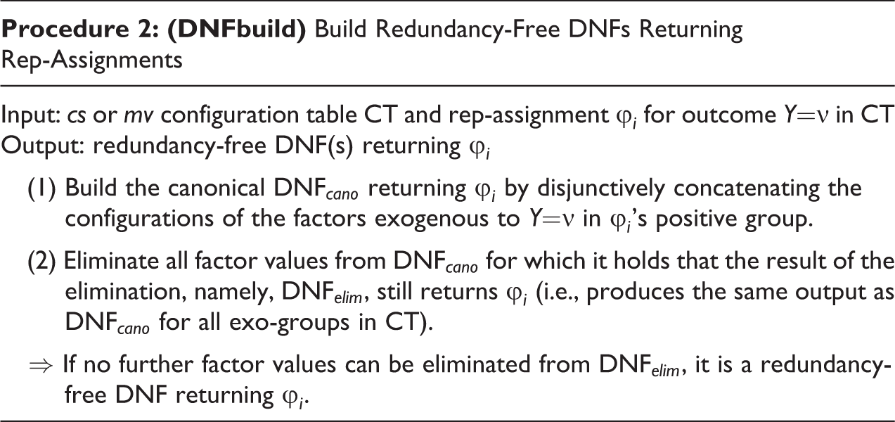
We end this section by assembling the steps building DNFs returning rep-assignments in procedural form, which we label DNFbuild, for short:

Procedure 2: (DNFbuild) Build Redundancy-Free DNFs Returning Rep-Assignments

Input: $cs$ or $mv$ configuration table $\text{CT}$ and rep-assignment ${\text{φ}}_i$ for outcome Y= $\nu$ in $\text{CT}$ Output: redundancy-free DNF(s) returning ${\text{φ}}_i$ (1) Build the canonical ${\text{DNF}}_{\mathrm{cano}}$ returning ${\text{φ}}_i$ by disjunctively concatenating the configurations of the factors exogenous to Y= $\nu$ in ${\text{φ}}_i$ ’s positive group.(2) Eliminate all factor values from ${\text{DNF}}_{\mathrm{cano}}$ for which it holds that the result of the elimination, namely, ${\text{DNF}}_{\mathrm{elim}}$ , still returns ${\text{φ}}_i$ (i.e., produces the same output as ${\text{DNF}}_{\mathrm{cano}}$ for all exo-groups in $\text{CT}$ ).⇒ If no further factor values can be eliminated from ${\text{DNF}}_{\mathrm{elim}}$ , it is a redundancy-free DNF returning ${\text{φ}}_i$ .

In case of $cs$ and $mv$ configuration tables, all ${\text{φ}}_i$ ’s have a canonical DNF, which is efficiently built by step (1) of DNFbuild. Step (2), by contrast, involves some intricacies. The reason is that different orders in which factor values are eliminated from DNF_cano may result in different redundancy-free DNFs. Generating all of these DNFs can be done more or less efficiently, but the running time of all algorithms that solve this problem grows exponentially with the number of factors and the number of values these factors can take. The cnaOpt package, which we use in the replication script, provides an algorithm called ereduce to generate all redundancy-free forms of DNF_cano. ¹² In the end, what matters for our current purposes is not the concrete implementation of step (2) but the fact that DNFbuild is guaranteed to find a redundancy-free DNF ${\Phi }_{rf}$ of every con-cov optimum $〈h,k〉$ . The equivalence ${\Phi }_{rf}\leftrightarrow Y$ = $\nu$ then amounts to a CCM model accounting for Y= $\nu$ with consistency h and coverage k. That is, in case of $cs$ and $mv$ data, there exists a CCM model for every con-cov optimum.

Fuzzy-set Data

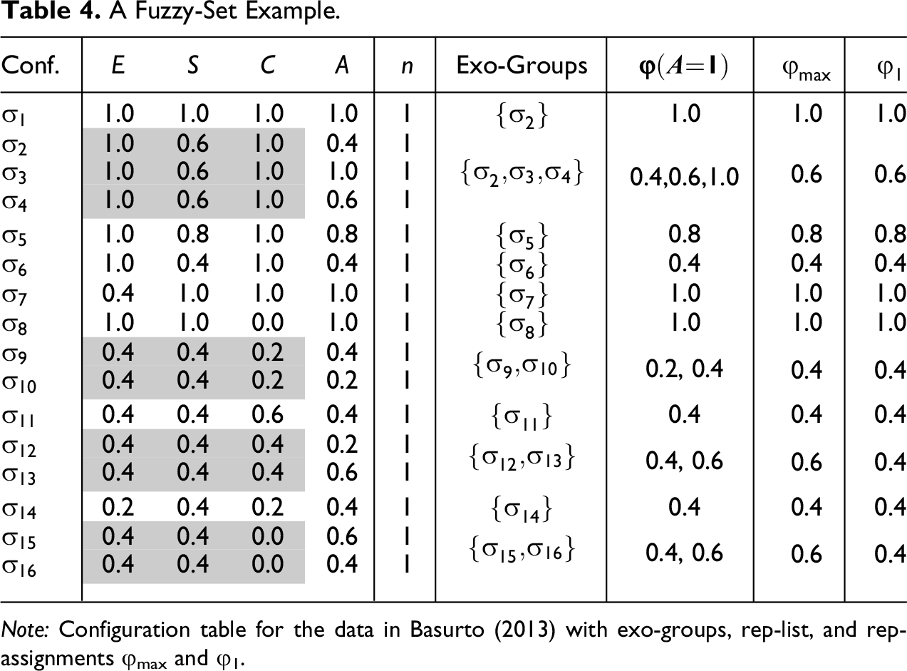
This section, first, applies ConCovOpt to $fs$ data and, second, shows that there is no guarantee that actual CCM models exist for every con-cov optimum in $fs$ data and that calculating con-cov optima for $fs$ data is more computationally demanding than for $cs$ and $mv$ data. As background for this discussion, we choose the study by Basurto (2013) who analyzes the autonomy among local institutions for biodiversity conservation in Costa Rica. The study aims to identify causes of, on the one hand, the emergence of autonomy between 1986 and 1998 and, on the other, the endurance of that autonomy between 1998 and 2006. Basurto investigates three groups of potentially causally relevant factors: local, national, and international ones. In what follows, we focus on the local influence factors of high local communal involvement through direct employment (E), high local direct spending (S), and co-management with local or regional stakeholders (C), and we concentrate on the outcome of endurance of high local autonomy (A), with 0 representing “no” and 1 “yes” for all factors (Basurto 2013:577). The data cover 16 Costa Rican biodiversity conservation programs; the factors are calibrated on a membership scale with increments of 0.2.

As input to ConCovOpt we, thus, use Basurto’s data (see the replication script) with $O=\{A$ = $1\}$ . In step (1), ConCovOpt builds the configuration table in Table 4. In this example, each case corresponds to exactly one configuration—which is not uncommon for $fs$ data. Since there, again, is only one outcome in $O$ , step (2) then builds one set of exo-groups, which are listed in column 4 of Table 4.

Table 4.

A Fuzzy-Set Example.

Conf.	E	S	C	A	n	Exo-Groups	$\phi (A$ = $1)$	${\text{φ}}_{\text{max}}$	${\text{φ}}_{\text{1}}$
${\text{σ}}_{\text{1}}$	1.0	1.0	1.0	1.0	1	${\text{{σ}}_{\text{2}}\text{}}$	1.0	1.0	1.0
${\text{σ}}_{\text{2}}$	1.0	0.6	1.0	0.4	1	${\text{{σ}}_{\text{2}}\text{,} {\text{σ}}_{\text{3}}\text{,} {\text{σ}}_{\text{4}}\text{}}$	0.4,0.6,1.0	0.6	0.6
${\text{σ}}_{\text{3}}$	1.0	0.6	1.0	1.0	1
${\text{σ}}_{\text{4}}$	1.0	0.6	1.0	0.6	1
${\text{σ}}_{\text{5}}$	1.0	0.8	1.0	0.8	1	${\text{{σ}}_{\text{5}}\text{}}$	0.8	0.8	0.8
${\text{σ}}_{\text{6}}$	1.0	0.4	1.0	0.4	1	${\text{{σ}}_{\text{6}}\text{}}$	0.4	0.4	0.4
${\text{σ}}_{\text{7}}$	0.4	1.0	1.0	1.0	1	${\text{{σ}}_{\text{7}}\text{}}$	1.0	1.0	1.0
${\text{σ}}_{\text{8}}$	1.0	1.0	0.0	1.0	1	${\text{{σ}}_{\text{8}}\text{}}$	1.0	1.0	1.0
${\text{σ}}_{\text{9}}$	0.4	0.4	0.2	0.4	1	${\text{{σ}}_{\text{9}}\text{,} {\text{σ}}_{\text{10}}\text{}}$	0.2, 0.4	0.4	0.4
${\text{σ}}_{\text{10}}$	0.4	0.4	0.2	0.2	1
${\text{σ}}_{\text{11}}$	0.4	0.4	0.6	0.4	1	${\text{{σ}}_{\text{11}}\text{}}$	0.4	0.4	0.4
${\text{σ}}_{\text{12}}$	0.4	0.4	0.4	0.2	1	${\text{{σ}}_{\text{12}}\text{,} {\text{σ}}_{\text{13}}\text{}}$	0.4, 0.6	0.6	0.4
${\text{σ}}_{\text{13}}$	0.4	0.4	0.4	0.6	1
${\text{σ}}_{\text{14}}$	0.2	0.4	0.2	0.4	1	${\text{{σ}}_{\text{14}}\text{}}$	0.4	0.4	0.4
${\text{σ}}_{\text{15}}$	0.4	0.4	0.0	0.6	1	${\text{{σ}}_{\text{15}}\text{,} {\text{σ}}_{\text{16}}\text{}}$	0.4, 0.6	0.6	0.4
${\text{σ}}_{\text{16}}$	0.4	0.4	0.0	0.4	1

Note: Configuration table for the data in Basurto (2013) with exo-groups, rep-list, and rep-assignments φ_max and φ₁.

The main peculiarity of $fs$ data is that configurations and outcomes are not merely instantiated or not instantiated in each case but instantiated with different set membership scores (i.e. to different degrees) in many different cases. One consequence is that there are often not only imperfect pairs but imperfect n-tuples, where n is the number of different membership scores an outcome has in an exo-group. An example is exo-group ${\text{{σ}}_{\text{2}}{\text{,σ}}_{\text{3}}{\text{,σ}}_{\text{4}}\text{}}$ in Table 4. Since A has three different membership scores in that group, namely, A= $0.4$ , A= $1.0$ , and A= $0.6$ , it corresponds to an imperfect triple. That the other three non-singleton exo-groups in Table 4 have only two elements is mere happenstance; $fs$ exo-groups can have as many members as there are values the outcome can take. Still, just as CCM models for other data types, models for $fs$ data have highest consistency and coverage if they reproduce the behavior of the outcome as closely as possible. That is, a DNF $\Phi$ of an $fs$ model $\Phi \leftrightarrow Y$ scores the higher on consistency and coverage, the closer the value of $\Phi$ comes to the value of Y for every exo-group.

Due to the instantiation by degrees in $fs$ data, however, the notion of reproducing the behavior of an outcome as closely as possible cannot be spelled out exactly as for $cs$ and $mv$ data. While a rep-assignment for the latter data types must reproduce the behavior of the outcome by only assigning one of two values, 0 or 1, a rep-assignment $\text{φ}$ for $fs$ data may assign many more values, namely, the minimum of the conjuncts’ scores in a conjunction and the maximum of the disjuncts’ scores in a disjunction. The values $\text{φ}$ can assign to a particular exo-group are constrained by the membership scores of the exogenous factors in that group. More specifically, as $\text{φ}$ is the output of a disjunction of conjunctions of factor values or their negations, it can only assign the membership scores of the positive or of the negated factors in that group, but no other values. To illustrate, take again the exo-group ${\text{{σ}}_{\text{2}}{\text{,σ}}_{\text{3}}{\text{,σ}}_{\text{4}}\text{}}$ , in which E= $1.0$ , S= $0.6$ , and C= $1.0$ . The conjunction E $\ast$ S $\ast$ C issues 0.6 for that group, namely, $\text{min}(1.0,0.6,1.0)$ ; correspondingly, e $\ast$ c and E $\ast$ C return 0.0 and 1.0, respectively, or s $\ast$ C outputs 0.4. But any value other than 0.0 (negation of E and C), 0.4 (negation of S), 1.0 (value of E and C), or 0.6 (value of S) cannot be assigned to that exo-group by $\text{φ}$ , meaning that those are $\text{φ}$ ’s possible values for that group. Hence, a rep-assignment $\text{φ}$ reproduces the behavior of an outcome as closely as possible if, and only if, it holds for every exo-group x that $\text{φ}$ assigns one of its possible values to x that comes as close as possible to the outcome’s membership scores in x. In the case of exo-group ${\text{{σ}}_{\text{2}}{\text{,σ}}_{\text{3}}{\text{,σ}}_{\text{4}}\text{}}$ that means that $\text{φ}$ reproduces the behavior of A as closely as possible iff it assigns one of 0.4, 0.6, or 1.0 to that exo-group (but not 0.0); or for exo-group ${\text{{σ}}_{\text{12}}{\text{,σ}}_{\text{13}}\text{}}$ $\text{φ}$ must assign either 0.4, which is equally close to A= $0.2$ and A= $0.6$ in that group, or 0.6, which is closest to A= $0.6$ . Sometimes the closest possible value of $\text{φ}$ exactly matches an outcome, sometimes it is far away from it. Sometimes only one of the possible values is closest to the outcome, sometimes multiple values are closest.

Based on this notion of reproducing the behavior of an outcome, step (3) builds the rep-list $\phi (A$ = $1)$ in Table 4 for Basurto’s data. From this list, 24 rep-assignments for outcome A are built in step (4). Just as in $cs$ and $mv$ data, the values of the rep-assignments and of the outcome are then plugged into the definitions for consistency and coverage in step (5)—this time, of course, using the fuzzy-set definitions ${\text{con}}^{fs}$ and ${\text{cov}}^{fs}$ in expression (2). After eliminating all rep-assignments inducing non-optimal scores, seven con-cov optima remain, which are plotted in Figure 2A with their con-cov products in Figure 2B.

Figure 2.

Plot A shows the seven con-cov optima for outcome A in the data of Basurto (2013) and the con-cov score of the published model ( $\blacksquare$ ) and Plot B shows the con-cov products of each optimum and of the published model. $▴$ is the con-cov maximum and ♦ the best optimum realizable by a CCM model.

Basurto (2013) chooses a consistency threshold of $0.79$ and produces an intermediate solution, equation (21), which coincides with QCA’s conservative solution. At that consistency threshold, QCA issues the two parsimonious solutions (22) and (23).

$\text{QCA}-\text{IS/CS:}\hspace{1em}C+E\ast S\leftrightarrow A\hspace{1em}\hspace{1em}\text{con}=0.79;\hspace{1em}\text{cov}=0.94,$

21

$\text{QCA}-\text{PS:}\hspace{1em}C + E\leftrightarrow A\hspace{1em} \text{con}=0.79;\hspace{1em}\text{cov}=0.94,$

22

$C + S\leftrightarrow A\hspace{1em} \text{con}=0.79;\hspace{1em}\text{cov}=\mathrm{0.96.}$

23

Contrary to our previous examples, these QCA models fall significantly short of a con-cov optimum, let alone a con-cov maximum. Moreover, the models are not robust under variations of the consistency threshold. But thanks to ConCovOpt, we now have concrete threshold settings at which to search for models with optimal fit. The con-cov maximum of $〈0.9,0.957〉$ ( $▴$ in Figure 2) is reached by the rep-assignment ${\text{φ}}_{\text{max}}$ in Table 4. It turns out, however, that neither QCA nor CNA nor CCubes find a model at the threshold setting $〈0.9,0.957〉$ , not even—as is possible in CNA and CCubes—if the consistency of individual disjuncts is allowed to fall short of 0.9. There simply does not exist a CCM model for outcome A at the con-cov maximum. This is not some idiosyncrasy of Basurto’s data. Con-cov optima for $fs$ data frequently do not have actual CCM models realizing them.

In a $cs$ and $mv$ configuration table, the configuration ${\Gamma }_i$ of exogenous factors in an exo-group $\left\{{\text{σ}}_i\right\}$ of an outcome Y is guaranteed not to be instantiated in any other exo-groups of Y. Hence, if Y is given in $\left\{{\text{σ}}_i\right\}$ , ${\Gamma }_i$ —properly freed of redundancies—can safely be included as a disjunct in a model of Y without affecting the model’s consistency in any exo-groups other than $\left\{{\text{σ}}_i\right\}$ . It is therefore possible to modularly build CCM models for every rep-assignment ${\text{φ}}_i$ along the lines of DNFbuild. The DNFbuild approach, however, does not work for $fs$ data, because if Y is an $fs$ outcome, the configuration ${\Gamma }_i$ in exo-group $\left\{{\text{σ}}_i\right\}$ may be instantiated with some non-zero membership in many other exo-groups. In consequence, including ${\Gamma }_i$ as a disjunct in a CCM model of Y is likely to affect the model’s consistency in exo-groups other than $\left\{{\text{σ}}_i\right\}$ . It may hence happen that a DNF only returns an optimal value for exo-group $\left\{{\text{σ}}_i\right\}$ provided it contains factor values that, at the same time, return a non-optimal value for another exo-group ${\text{{σ}}_j\}$ , meaning that no DNF returns optimal values for both $\left\{{\text{σ}}_i\right\}$ and $\left\{{\text{σ}}_j\right\}$ .

To make this (abstract problem) concrete, compare the exo-groups ${\text{{σ}}_{\text{9}}{\text{,σ}}_{\text{10}}\text{}}$ and ${\text{{σ}}_{\text{15}}{\text{,σ}}_{\text{16}}\text{}}$ in Table 4. The rep-assignment ${\text{φ}}_{\text{max}}$ assigns 0.4 to ${\text{{σ}}_{\text{9}}{\text{,σ}}_{\text{10}}\text{}}$ and 0.6 to ${\text{{σ}}_{\text{15}}{\text{,σ}}_{\text{16}}\text{}}$ . Given the membership scores E= $0.4$ , S= $0.4$ , and C= $0.2$ in ${\text{{σ}}_{\text{9}}{\text{,σ}}_{\text{10}}\text{}}$ , a DNF only returns 0.4 for ${\text{{σ}}_{\text{9}}{\text{,σ}}_{\text{10}}\text{}}$ if it includes E or S or E $\ast$ S as a disjunct. But E, S, and E $\ast$ S also return 0.4 for group ${\text{{σ}}_{\text{15}}{\text{,σ}}_{\text{16}}\text{}}$ , while ${\text{φ}}_{\text{max}}$ assigns 0.6 to that group. Given the membership scores E= $0.4$ , S= $0.4$ , and C= $0.0$ in ${\text{{σ}}_{\text{15}}{\text{,σ}}_{\text{16}}\text{}}$ , a DNF would have to include e or s or e $\ast$ s in order to return 0.6 for ${\text{{σ}}_{\text{15}}{\text{,σ}}_{\text{16}}\text{}}$ . But if those factor values are included, 0.6 is issued for ${\text{{σ}}_{\text{9}}{\text{,σ}}_{\text{10}}\text{}}$ , which again is not the value assigned by ${\text{φ}}_{\text{max}}$ . In sum, no DNF outputs 0.4 for ${\text{{σ}}_{\text{9}}{\text{,σ}}_{\text{10}}\text{}}$ and 0.6 for ${\text{{σ}}_{\text{15}}{\text{,σ}}_{\text{16}}\text{}}$ , meaning that no actual CCM model will realize ${\text{φ}}_{\text{max}}$ .

This problem is avoided if we do not require 0.6 to be issued for ${\text{{σ}}_{\text{15}}{\text{,σ}}_{\text{16}}\text{}}$ but 0.4, which indeed happens to be assigned by another rep-assignment, ${\text{φ}}_1$ (cf. Table 4), yielding the con-cov optimum $〈0.935,0.915〉$ . Moreover, it turns out that there exists an actual DNF also reproducing all other values of ${\text{φ}}_1$ . At a threshold setting of $〈0.93,0.91〉$ , both CNA and CCubes find the following model: ¹³

$\text{CNA/CCubes:}\hspace{1em}S\leftrightarrow A\hspace{1em}\hspace{1em}\text{con}=0.935;\hspace{1em}\text{cov}=\mathrm{0.915.}$

24

Apart from there being no guarantee that $fs$ con-cov optima are realizable by actual models, the $fs$ case also differs from ConCovOpt analyses of $cs$ and $mv$ data in its computational complexity. The most computationally costly step of ConCovOpt is step (5), which calculates fit scores of rep-assignments. The more rep-assignments are entailed by a configuration table, the more time-consuming that calculation. In case of $cs$ and $mv$ data, the amount of rep-assignments is only a function of the number of non-singleton exo-groups, which, in turn, is a function of the number of imperfect pairs in the data. ¹⁴ A $cs$ or $mv$ DNF optimally reproduces the behavior of an outcome Y= $\nu$ in every singleton exo-group by returning 1 if Y takes the value $\nu$ in that exo-group or 0 otherwise. In consequence, no rep-assignment needs more than one value assignment to optimally capture the outcome’s behavior in singleton exo-groups. By contrast, it might be that multiple output values of an $fs$ DNF reproduce the outcome’s value in a singleton exo-group ${\text{{σ}}_i\}$ equally optimally. This happens if the outcome’s value is not itself among the possible values of the exogenous factors in ${\text{{σ}}_i\}$ and multiple of those possible values are equally close to the outcome’s value. In that case, multiple rep-assignments result from the singleton exo-group ${\text{{σ}}_i\}$ . It follows that the number of rep-assignments does not only grow with the number of imperfect configurations but also with the number of cases. This, in combination with the fact that rep-assignments may assign more than two values to exo-groups, yields that exhaustively searching for con-cov optima is much more computationally demanding for $fs$ data.

Our R implementation of ConCovOpt can calculate the fit scores of about 10 million rep-assignments in reasonable time. For $cs$ and $mv$ data that means that ConCovOpt can process data of any sample size with up to 23 imperfect pairs. In case of $fs$ data, however, the computational limit tends to be reached at intermediate-N sample sizes of 70–80 cases with 10–15 imperfect n-tuples (see the replication script for a corresponding benchmark test). To calculate con-cov optima also for large-N $fs$ data, heuristics are called for. In our R implementation, we use an approximation method that induces ConCovOpt to calculate fit scores only for rep-assignments with values closest to the outcome’s median. This is an efficient approach for finding many, but possibly not all, con-cov optima. Based on this approximation method, large-N $fs$ data of up to 2,000 cases become processable.

Overall, even though heuristics are needed to calculate con-cov optima for large-N data and there may be no models realizing certain optima, processing $fs$ data by ConCovOpt prior to actual CCM analyses has a considerable payoff. It identifies a set of consistency and coverage settings at which concrete models can be searched in a goal-oriented manner. Without applying ConCovOpt to Basurto’s data, we would have been in the dark as to where to search for optimal models and would have had to proceed in an inefficient trial-and-error manner. With ConCovOpt, we straightforwardly found model (24), which has significantly better fit than Basurto’s published model (21). Moreover, that fit improvement substantively alters the causal conclusions to be drawn from Basurto’s (2013) study. A causal interpretation of equation (24) suggests that the endurance of autonomy only depends on local direct spending. Contrary to Basurto’s findings, there is no evidence in his data that the other exogenous factors might be difference-makers of autonomy endurance as well.

Discussion

We end this article by putting ConCovOpt into proper methodological perspective. Most importantly, ConCovOpt is not intended as a tool for a “simple hunt for high values of consistency and coverage” (Schneider and Wagemann 2012:148). As emphasized in the Introduction section, there are other criteria of model selection. That is, high consistency and coverage are one asset of a model among others, and models with higher consistency and coverage should not be unequivocally preferred if they are outperformed by rival models in other respects.

What is more, the problem of model overfitting is still underinvestigated in configurational causal modeling, and there is ample evidence that CCMs have a strong tendency to overfit if they are induced to do so by overly high consistency and coverage thresholds (see, e.g., Arel-Bundock 2019; Braumoeller 2015). One (heuristic) indication that overfitting might be taking place is that the complexity of resulting models increases disproportionally to their increase in model fit. This phenomenon regularly occurs if CCMs are “forced” to build models reaching con-cov maxima—an example is provided in the replication script. What would hence be needed is a tool analogous to, say, the Akaike Information Criterion in statistical modeling that strikes a balance between model fit and simplicity. A general preference of models reaching con-cov maxima is blind and hazardous.

Still, we have discussed various examples in this article for which ConCovOpt has helped to significantly increase the model fit without an increase in model complexity, thus steering clear of overfitting dangers. Moreover, systematically scanning the model space at optimal consistency and coverage scores has led to the resolution of model ambiguities in case of Verweij and Gerrits’s (2015) as well as Basurto’s (2013) data; and it has even called into question the causal interpretability of a whole data set, namely, in case of the study by Britt et al. (2000). All of this shows that rendering con-cov optima and maxima transparent may importantly affect the causal conclusions drawn from configurational data.

Hence, ConCovOpt is intended as a tool for systematically exploring the space of CCM models at optimal consistency and coverage scores. In recent years, the awareness in the CCM literature has grown that the space of viable models for analyzed data may be larger than anticipated (cf., e.g., Baumgartner and Thiem 2017). When the data quality is very high, meaning when there are no imperfect pairs (or n-tuples), uncovering the whole model space is a matter of applying the relevant CCM once, at one determinate threshold setting. But in the presence of imperfect pairs, multiple CCM-runs at various threshold settings are needed. Slight changes in thresholds may greatly change the models and there may be no systematicity in how threshold changes affect model changes. ConCovOpt efficiently uncovers con-cov optima and maxima prior to the application of CCMs. This information makes it possible to apply CCMs by directly constraining them towards optimal thresholds, without having to go through a whole array of threshold settings. Also, it can be determined how close actually obtained models come to con-cov optima and whether the obtained models exhaust the space of con-cov optima or whether further models should be searched at different settings.

All of this is of importance not only to analysts primarily interested in data-driven causal inference but also to analysts (of which there are many) viewing CCMs as tools for inferences primarily rooted in available case knowledge. When it comes to model selection, all types of CCM analysts have to take model fit into account. Even the analyst who wants to choose models based on case knowledge does not draw causal inferences from case knowledge alone. Rather, she analyzes data by means of a CCM in order to be presented with a set of models to choose from. The ultimate purpose of ConCovOpt and DNFbuild is to contribute to the completeness of that set.

In sum, models reaching con-cov optima will sometimes turn out to be the best models overall, sometimes not, and sometimes they will be of methodological interest even without being causally interpreted. But in one way or another, transparency on the model space at consistency and coverage optima is univocally valuable for configurational causal modeling.

Supplemental Material

Supplemental Material, sj-r-1-smr-10.1177_0049124121995554 - Optimizing Consistency and Coverage in Configurational Causal Modeling

Supplemental Material, sj-r-1-smr-10.1177_0049124121995554 for Optimizing Consistency and Coverage in Configurational Causal Modeling by Michael Baumgartner and Mathias Ambühl in Sociological Methods & Research

References

1.
AmbühlMathiasBaumgartnerMichael. 2020a. cna: Causal modeling with Coincidence Analysis. R Package Version 3.0.1. Retrieved March 3, 2021, https://cran.r-project.org/package=cna.
2.
AmbühlMathiasBaumgartnerMichael. 2020b. cnaOpt: Optimizing Consistency and Coverage in Configurational Causal Modeling. R Package Version 0.2.0. Retrieved March 3, 2021, https://cran.r-project.org/package=cnaOpt.
3.
Arel-BundockVincent. 2019. “The Double Bind of Qualitative Comparative Analysis.” Sociological Methods & Research. 1–20. doi: 10.1177/0049124119882460.
4.
BasurtoXavier. 2013. “Linking Multi-level Governance to Local Common-Pool Resource Theory Using Fuzzy-set Qualitative Comparative Analysis: Insights from Twenty Years of Biodiversity Conservation in Costa Rica.” Global Environmental Change23(3):573–87.
BaumgartnerMichaelAmbühlMathias. 2020. “Causal Modeling with Multi-value and Fuzzy-set Coincidence Analysis.” Political Science Research and Methods8(3):526–42.
7.
BaumgartnerMichaelFalkChristoph. 2019. “Boolean Difference-making: A Modern Regularity Theory of Causation.” The British Journal for the Philosophy of Science. doi: 10.1093/bjps/axz047.
BraumoellerBaer F.2015. “Guarding against False Positives in Qualitative Comparative Analysis.” Political Analysis23(4):471–87.
10.
BrittDavid W.RisingerSamantha T.MillerVirginiaMansMary K.KrivcheniaEric L.EvansMark I.. 2000. “Determinants of Parental Decisions after the Prenatal Diagnosis of Down Syndrome: Bringing in Context.” American Journal of Medical Genetics93(5):410–16.
11.
CronqvistLasseBerg-SchlosserDirk. 2009. “Multi-value QCA (mvQCA).” Pp. 69–86in Configurational Comparative Methods: Qualitative Comparative Analysis (QCA) and Related Techniques, edited by RihouxB.RaginC. C.. Thousand Oaks, CA: Sage.
12.
DusaAdrian. 2018. “Consistency Cubes: A Fast, Efficient Method for Exact Boolean Minimization.” The R Journal10(2):357–70.
13.
GiugniMarcoYamasakiSakura. 2009. “The Policy Impact of Social Movements: A Replication through Qualitative Comparative Analysis.” Mobilization: An International Quarterly14(4):467–84.
14.
GraßhoffGerdMayMichael. 2001. “Causal Regularities.” Pp. 85–114in Current Issues in Causation, edited by SpohnW.LedwigM.EsfeldM.. Paderborn, Germany: Mentis.
LewisDavid. 1973. “Causation.” Journal of Philosophy70:556–67.
17.
MackieJohn Leslie. 1974. The Cement of the Universe. A Study of Causation. Oxford, England: Clarendon Press.
18.
RaginCharles. 1987. The Comparative Method. Berkeley: University of California Press.
19.
RaginCharles. 2006. “Set Relations in Social Research: Evaluating Their Consistency and Coverage.” Political Analysis14:291–310.
20.
RaginCharles. 2008. Redesigning Social Inquiry: Fuzzy Sets and Beyond. Chicago: University of Chicago Press.
21.
RihouxBenoîtMeurGisèle De. 2009. “Crisp-set Qualitative Comparative Analysis (csQCA).” Pp. 33–68in Configurational Comparative Methods: Qualitative Comparative Analysis (QCA) and Related Techniques, edited by RihouxB.RaginC.. Thousand Oaks, CA: Sage.
22.
SchneiderCarsten Q.WagemannClaudius. 2012. Set-theoretic Methods: A User’s Guide for Qualitative Comparative Analysis (QCA) and Fuzzy-sets in the Social Sciences. Cambridge, England: Cambridge University Press.
23.
SuppesPatrick. 1970. A Probabilistic Theory of Causality. Amsterdam, the Netherlands: North Holland.
ThiemAlrikBaumgartnerMichaelBolDamien. 2016. “Still Lost in Translation! A Correction of Three Misunderstandings between Configurational Comparativists and Regressional Analysts.” Comparative Political Studies49:742–74.
26.
VerweijStefanGerritsLasse M.. 2015. “How Satisfaction Is Achieved in the Implementation Phase of Large Transportation Infrastructure Projects: A Qualitative Comparative Analysis into the A2 Tunnel Project.” Public Works Management & Policy20(1):5–28.
Supplementary Material
Please find the following supplemental material available below.
For Open Access articles published under a Creative Commons License, all supplemental material carries the same license as the article it is associated with.
For non-Open Access articles published, all supplemental material carries a non-exclusive license, and permission requests for re-use of supplemental material or any part of supplemental material shall be sent directly to the copyright owner as specified in the copyright notice associated with the article.