Life-Course-Sensitive Analysis of Group Inequalities: Combining Sequence Analysis With the Kitagawa–Oaxaca–Blinder Decomposition

Abstract

Processes that unfold over individuals’ life courses are often associated with inequalities later in life. The literature lacks methodological approaches to analyze inequalities in outcomes between groups, for example, between women and men, in a life-course-sensitive manner. We propose a combination of methods—of sequence analysis, which enables us to study the multidimensional complexity of life courses with Kitagawa–Oaxaca–Blinder decomposition. This approach allows us to distinguish the share of inequalities between groups that is due to group-specific life courses from the share that is due to group-specific returns to similar life courses. We illustrate the combination of the two methods by analyzing work–family life courses and gender pension gaps in Italy and Germany. Our contribution is to systematically compare possible core analytical choices when combining typologies derived using sequence analysis with the Kitagawa–Oaxaca–Blinder decomposition. For future applications, we propose a set of practical guidelines for sequence analysis–Kitagawa–Oaxaca–Blinder decomposition.

Introduction

What processes link earlier life courses to group-specific inequalities later in life? Are there differences across welfare states? To address these and related questions, we propose a stepwise combination of sequence analysis (SA) and Kitagawa–Oaxaca–Blinder (KOB) decomposition, and systematically compare different possibilities for core analytical choices. In the process, we highlight advantages and limitations and derive a set of practical guidelines for combining the two methods.

Sequence analysis has become the standard method in the social sciences for analyzing trajectories of several categorical states —that is, how these states develop over a certain time (Liao et al. 2022). The most prominent of these states are work and family life courses. SA is used to identify, categorize and visualize similar life-course patterns in cluster-based typologies. Multichannel sequence analysis (MSA) is a special form of SA that is used to describe how events in multiple domains (e.g., employment and family life) unfold jointly (Gauthier et al. 2010; Pollock 2007). MSA's advantages include its capacity to simultaneously consider the occurrence and duration of certain life-course states, their timing, and their sequencing in more than one life domain. A typical example is the association between parenthood (family domain) and employment (work domain): parents often leave the labor force to care for their children. To date, life-course typologies emerging from SA and cluster analysis have been used as dependent or independent variables in regression models (e.g., Madero-Cabib and Fasang 2016; Möhring and Weiland 2021; Riekhoff and Järnefelt 2017). Yet, these existing SA designs have not assessed whether group inequalities in outcomes, such as the gender pension gap (GPG), arise from group-specific compositional differences in life courses or from group-specific returns to similar life courses. For example, does the GPG mainly result from men and women experiencing entirely different life courses or from men and women receiving differential pension returns to similar life courses?

KOB decomposition is the method of choice to estimate group-specific inequalities in outcomes, for example, gender wage gaps (Kunze 2018). Going beyond regression analyses, KOB decomposition reveals what part of the gap is due to differences in mean characteristics between groups and what part is due to group differences in returns to the same characteristics. However, previous studies have heavily relied on summary indicators (e.g., years of full-time work) or “point-in-time” indicators to account for individual experiences over the life course. Such measures simplify life-course complexities, such as the timing, ordering, or co-occurrence of events over the life course (Halpern-Manners et al. 2015). We propose combining the strengths of SA and KOB to provide a life-course-sensitive analysis of group inequalities. Specifically, a combination of SA and KOB captures the extent to which gender gaps are related to (a) gender-specific life-course clusters (i.e., compositional differences), or (b) unequal rewards for men and women with similar life courses who are classified in the same life-course cluster (i.e., differential returns).

We illustrate the SA–KOB decomposition by analyzing the GPG in Italy and West Germany for the years 2006–2015 and the birth cohorts 1911–1950 using data from the Survey of Health, Ageing and Retirement in Europe (SHARE). By comparing Italy and (West) Germany, we highlight the added value of the proposed procedure for comparative welfare state studies. Germany and Italy share characteristics typical of conservative welfare states but have different pension systems. So far, empirical studies have typically decomposed the GPG based on one-dimensional summary measures and focused on the employment sphere (e.g., Even and Macpherson 2004; Zhao and Zhao 2018). However, life-course research shows that work and family life courses and their combinations are highly gender specific and vary across welfare states (e.g., Fasang and Aisenbrey 2022; Komp-Leukkunen 2019; Madero-Cabib and Fasang 2016; Tosi and Grundy 2019). The literature currently lacks an account of work–family life course relations that uncovers gender-specific inequalities in later life outcomes, such as the GPG (Allmendinger, Brückner and Brückner 1992; Ginn, Daly and Street 2001). To address this in the context of the SA–KOB application, we make use of MSA in our illustration and provide guidelines that can be used to decide whether to cluster different life-course domains separately based on single-channel SA or account for their relationship by clustering them jointly using MSA. Only a few studies have used SA and regression analysis to identify typologies of life courses and relate them to women's pension incomes (Madero-Cabib and Fasang 2016; Möhring and Weiland 2021; Tophoven and Tisch 2016). To date, no study has combined SA with decomposition methods to identify the share of GPGs due to compositional differences in life courses between men and women or differential returns to similar life courses. ¹ Combining SA and decomposition can provide new insights on a broad range of related questions regarding how trajectories of categorical states are associated with subsequent group inequalities. To combine the two methods, we first run sequence and cluster analyses to identify a typology of prevalent life courses. We then use this typology as a covariate in a KOB decomposition of group differences in an outcome, here gender gaps in pensions.

Our contribution is therefore twofold. First, we introduce and systematically compare different possibilities in core analytical choices when combining SA and KOB to derive a set of general guidelines for applying SA–KOB decomposition. Second, our empirical example generates new insights into the association between gendered life courses and the GPG, with implications for other fields of application. Specifically, we show that a substantial proportion of the GPG is due to the temporal interdependence between the occurrence of certain family transitions (to partnership and parenthood) and transitions from different types of labor-market participation to unpaid care work. However, these transitions only arise in life course clusters typical for women. MSA captures this link over time between life-course spheres overlooked by previous research, which has focused on the characteristics of labor-market participation. SA–KOB decomposition also overcomes limitations of previous GPG studies, which had to restrict the number of measures of working lives used to avoid multicollinearity.

Both SA and KOB are descriptive methods, and their combination does not allow any causal inference. Yet, the distinction between compositional and return effects of life courses on later life outcomes has implications for life-course theory and social policy. The SA–KOB combination offers more detailed descriptive findings that can support or refute theoretical propositions on processes of accumulation over the life course. For instance, different mechanisms are likely to drive compositional or return effects to life courses, as we elaborate below, and this has immediate policy implications. Specifically, reducing compositional differences in life courses would likely require policy measures directed at early and middle adulthood, whereas adjusting pension regulations might alleviate group differences in pension returns to similar life courses. The combination of SA and KOB can easily be applied to any outcome linked to processes of accumulation over the life-course that are group-specific, for example, wealth or health gaps by gender or race.

We first introduce our application and then discuss necessary steps in SA and KOB in detail. As we move through the discussion of the various steps, we outline practical guidelines for applications. Before we discuss the SA–KOB results, we first replicate the most popular way of analyzing GPGs so far, that is decomposing them based on life course summary measures. Last, we compare the results of KOB based on life course summary measures and SA–KOB and conclude with a discussion of the main contributions of SA–KOB.

Illustrative Application: Life Courses and Gender Pension Gaps in Germany and Italy

Gendered Life Courses and Retirement Systems

Family life courses are more strongly associated with women's pension income than with men's (e.g., Fasang 2010; Fasang, Aisenbrey, and Schomann 2013; Hofmeister, Blossfeld, and Mills 2006; Krüger and Levy 2001; Meyer and Pfau-Effinger 2006; Muller, Hiekel, and Liefbroer 2020). Family and care responsibilities are “key individual determinant[s] of women's employment” (Zagel and Van Winkle 2020: 3), and the literature documents employment and earnings penalties of marriage and motherhood that vary across welfare states (e.g., Aisenbrey, Evertsson, and Grunow 2009; Arntz, Dlugosz, and Wilke 2017; Boeckmann, Misra, and Budig 2015; Gangl and Ziefle 2009). Cumulative advantage or disadvantage (CAD) in life-course theory (Dannefer 2003) expresses “that the advantage of one individual or group over another grows (i.e., accumulates) over time” (DiPrete and Eirich 2006: 272), leading to increasing within-cohort inequality that culminates in old age (Dannefer 1987). In the tradition of CAD “[t]he gender gap in pensions can be understood as the sum of gender inequalities over a lifetime, including differences in the life-course (motherhood penalty), segregated labour market and gendered social norms and stereotypes more generally” (European Institute for Gender Equality 2015: 4). Therefore, both employment and family life courses have to be considered when analyzing gender gaps in pension income. Institutional and cultural contexts foster or discourage certain gender arrangements and thus shape gendered life courses and outcomes (Elder, Johnson, and Crosnoe 2003; Krüger and Levy 2001; Pfau-Effinger 1998; Rosenfeld, Trappe, and Gornick 2004). Moreover, pension systems reward certain life courses more than others (Ginn et al. 2001). Most pension systems assume continuous full-time employment as the norm (Leitner 2001) and disregard the gendered division of labor.

A gender-sensitive analysis of pension inequalities requires researchers to consider all factors shaping access to and amounts of pension income (Ginn et al. 2001; Jefferson 2009). Regarding access to pension claims, eligibility rules, age thresholds, and mechanisms for considering time spent doing unpaid care work are particularly relevant for women (Ginn et al. 2001). A usual qualifying condition is the minimum length of contribution, which systematically excludes individuals with discontinuous employment records and thus disproportionately affects women (Leitner 2001). Regarding the amount, overall redistributive elements tend to augment women's pension incomes (Ginn 2004; Vlachantoni 2012). Conversely, earnings-related contributions and less progressive pension systems are disadvantageous for women (Grech 2013; Horstmann et al. 2009; Samek Lodovici et al. 2011). Care benefits and the upgrading of part-time work in pension entitlement further elevate women's pension income (Möhring 2018). Because women have more interrupted work lives, lower earnings, and limited access to occupations that guarantee generous occupational pension schemes, they often find that personal pensions ² —which are gaining importance in most European countries—yield lower returns or are not viable in the first place (Ginn 2003, 2004; Ginn and Arber 1996; Jefferson 2009; Möhring 2018).

Empirical Evidence on Gender Pension Gaps

Most studies have decomposed the GPG based on a set of individual-level characteristics, including retrospective information on labor-market attachment, operationalized as the sum of years individuals spent in a certain employment status over their life course (Bardasi and Jenkins 2010; Bettio, Tinios, and Betti 2013; Bonnet, Meurs, and Rapoport 2020; Cordova, Grabka, and Sierminska 2022; Even and Macpherson 2004; Ezeyi and Vujic 2017; Hänisch and Klos 2014; König, Johansson, and Bolin 2019; Levine, Mitchell, and Phillips 1999; Nolan et al. 2019; Veremchuk 2020; Zhao and Zhao 2018). Table A1 in the supplemental material provides an overview of decomposition analyses of GPGs. Most of the studies on public pensions or total pension income have stressed that gender differences in labor-market attachment are among the main explanatory factors for GPGs (Bonnet et al. 2020; Even and Macpherson 2004; Frommert and Strauß 2013; Hänisch and Klos 2014; Levine et al. 1999; Nolan et al. 2019). The few studies that have included family life-course indicators (Table A1 in the supplemental material) show that gender differences in marriage rates are related to higher GPGs, whereas the higher share of widowed women compared to men is related to lower GPGs in most countries (e.g., Hänisch and Klos 2014; Veremchuk 2020). Two studies support the idea that much of the GPG is due to gender differences in returns to marital status and fertility, i.e., women experience pension penalties for marriage and parenthood but men enjoy pension premiums (Bardasi and Jenkins 2010; Ezeyi and Vujic 2017).

Other studies have focused on women's pensions or gender inequalities in pension incomes by applying OLS regressions instead of decomposition techniques. They have incorporated the life course perspective by including similar summary measures as the decomposition literature as well as composite indicators, for instance on “career volatility” (Möhring 2015: 11) or career types (Sefton et al. 2011). Evandrou, Falkingham, and Sefton (2009) and Fasang et al. (2013) found strong associations between summary measures of family history and women's later life income, partly even after controlling for socioeconomic status and employment history.

Madero-Cabib and Fasang (2016) analyzed (gendered) old age income inequalities using MSA to identify typologies of work and family life courses. Findings indicated that, in West Germany and Switzerland, female-dominated life courses are much less well-rewarded than men's standard life courses (characterized by continuous full-time employment, being married, and having at least two children). More recently, Möhring and Weiland (2021) have taken a couple perspective and shown for Germany that women's old-age income is highest for women in dual-earner couple life courses and lowest for women in male-breadwinner partnerships, though this association weakens when controlling for the number of children and the share of childcare over women's life courses. Focusing on the association between employment life courses and public pension claims in Germany, Tophoven and Tisch (2016) found that women with unstable or interrupted work life courses had lower pension claims than those with relatively stable full-time or part-time trajectories. However, neither Möhring and Weiland (2021) nor Tophoven and Tisch (2016) included family life courses in the SA step.

Italy and West Germany

Italy and West Germany ³ are two examples of gender-conservative welfare state systems and have among the highest GPGs in Europe (Hammerschmid and Rowold 2019). While the pension systems are different, both are described as Bismarckian models that are particularly disadvantageous for women due to the tight link between earnings and pension benefits (Corsi and D’Ippoliti 2009; Fasang 2010; Horstmann et al. 2009; Samek Lodovici et al. 2011).

Family Policies and Gender Norms

In the twentieth century, West Germany was an ideal-typical gender-conservative welfare regime (Trappe, Pollmann-Schult, and Schmitt 2015). A significant policy shift toward more gender equality started at the beginning of the 2000s; however, this was not relevant for our study cohorts, who had long completed their active family formation at this time. In the familial Italian welfare state, benefits have traditionally been structured around family units rather than individuals (Saraceno 1994), and the state has relied on family members (namely women) to provide care work (Hofmeister et al. 2006). Family policies were similar in West Germany and Italy for our study cohorts. Table S1 in the Supplementary Materials displays a summary of family policies and gender norms in the two countries. For instance, childcare in both countries only recently started to be publicly funded and regulated for children aged three or older, and gender and family norms were similarly traditional in the 1980s and 1990s. In both countries, female labor force participation was very low in 1990, but the rate in Germany was higher due to female part-time employment. Unlike Germany, Italy has no legacy of part-time work (Hofmeister et al. 2006). Additionally, joint taxation of married spouses and limited daycare opening hours in West Germany encouraged women to perform part-time work (Rosenfeld et al. 2004). Apart from women's higher access to part-time work in Germany, we expected to find similar gender differences in typical life courses for women and men in these two traditional welfare states and normative contexts.

Pension Systems

Table S2 in the Supplementary Materials summarizes the pension systems. Both pension systems are Bismarckian, but the Progressivity Index suggests that the Italian public pension system is overall less redistributive than the German one. To qualify for old age pensions, individuals in Italy must have a much higher contribution record (20 years vs. 5 years), which is more difficult for women to reach. ⁴ This might explain why 35% of Italian women but only 9% of West German women aged 65 + do not receive any own pension income. Even though both public systems provide benefits for child (and elderly) care, women with low incomes particularly benefit from child benefits in Germany. Unlike in Italy, in Germany these claims are based on the overall average income for the respective year and not on previous individual income. Thus, care benefits in Germany do not reproduce previous (gendered) labor-market disadvantages (Horstmann et al. 2009). Moreover, upon divorce, partners split their pension entitlements in Germany, but they do not do so in Italy—that is, entitlements are transferred from the partner with the higher claim to the one with the lower claim, which generally benefits women (Kreyenfeld, Schmauk, and Mika 2022). Finally, women in Germany benefit slightly more from the redistributive elements in the pension system, whereas men in Italy tend to be favored (suggested by the gender gap in replacement rate). At the same time, regressive personal pensions that tend to disadvantage women are more widespread in Germany than in Italy. Because public pensions are the main source of total pension income in both countries, we expect gender inequalities over the life course to be slightly more reproduced in the Italian pension system. In sum, we expect that compositional differences in life courses will account for sizeable shares of the GPG in both countries. However, we expect the share accounted for by compositional differences and return effects to similar life courses in the pension system to be larger in Italy than in Germany.

Data, Sample, and Variables

The data came from the SHARE (Börsch-Supan et al. 2013). ⁵ We used Wave 5 as a base sample of individuals aged 65 or older at the year of interview and merged respondents from Waves 2, 4, and 6 who were not surveyed in Wave 5 to increase case numbers in the analytical sample. The survey years spanned 2006 to 2015 (see Table A2 in the supplemental material). We combined the cross-sectional information in the analytical sample with retrospective annual data on family and work life courses from age 18 to 65 included in SHARELIFE, collected in 2008–2009 and 2017 (Brugiavini et al. 2019). ⁶

The analytical sample included individuals aged 65 and older and excluded respondents: (i) with missing information on controls and annual pension income; (ii) who were part of the labor force and in receipt of a salary or unemployment benefits at the time of the interview; or (iii) who had entirely missing retrospective data. We retained nonemployed respondents who reported work that could be classified as spare-time work or similar to keep retirees in need of additional income in the sample.

Pension income was specified as individual income from public, occupational, and private pensions based on independent own achievements. Income sources that were derived from other individuals, most importantly survivor pensions (see Table A3 in the supplemental material) were excluded, as they were associated with economic dependence and a loss of autonomy (e.g., Ginn et al. 2001).

Women were more likely than men to not receive pension income. We retained respondents who reported to receive no pension income and assigned them a pension income of 0. Our analysis thereby broadly covers the entire population 65+ . We used the absolute annual pension incomes and adjusted for purchasing power. We only considered regular payments (i.e., no lump sum payments, which played a marginal role in Germany and Italy). We further top-coded the highest 1% annual pension income with the 99^th percentile.

Analytical Strategy

Step I: Sequence Analysis

Overview of Sequence Analysis

Over the last twenty years, sequence analysis (SA) has become a key analytical tool for analyzing trajectories of categorical states in the social sciences, particularly in the field of life-course research (Abbott 1995; Liao et al. 2022; MacIndoe and Abbott 2004). The standard SA workflow pursues an exploratory approach to uncover regularities in temporal processes by, first, operationalizing sequences of categorical states that capture a temporal process of interest (e.g., educational or employment trajectories) and then using data-reduction techniques such as cluster analysis to identify the most typical empirical realization of that process. Typically, sequence analysis is used to calculate pairwise distances between all individuals in a sample to determine sequence similarity. This pairwise dissimilarity matrix captures the extent to which each sequence is similar to any other one in the sample. Similarity is understood as the cost of the operations computed to transform one sequence into another. Operations include the insertion, deletion, or substitution of states along the sequences: this is the basic optimal matching strategy, as introduced by Abbott and Hrycak (1990; see Studer and Ritschard 2016 for an overview of distance metrics). The sequence dissimilarity matrix is used in a cluster analysis to identify typologies of sequence clusters. The clusters can be used as dependent or independent variables in a regression framework to link them to baseline individual characteristics or to an outcome. For a detailed and step-wise introduction to SA, including instructions for coding in the TraMineR module in R (Gabadinho et al. 2011) see Raab and Struffolino (2022).

Single Versus Multichannel Sequence Analysis

To address life-course-related questions, researchers may need to account for parallel processes in different life domains—for example, employment and family formation. There are several strategies used to construct a joint multidomain typology. The most popular consists of the computation of a joint dissimilarity matrix based on costs derived additively from domain costs (Gauthier et al. 2010; Pollock 2007). This is referred to as MSA (see Piccarreta 2017 and Raab and Struffolino 2022 for an overview and Ritschard, Liao, and Struffolino 2023 for a critical review).

Both single-channel SA—that is, the application of SA to one life-course domain (e.g., work or family)—and multichannel SA—that is, the application of MSA to account for several domains simultaneously (e.g., work and family)—can be combined with KOB. The question of whether to apply single or multichannel SA depends on the research question and the data characteristics. There are three options for combining single-channel SA and KOB. The first applies to research questions that focus on one domain; in this case, clusters are generated for the single domain of interest and they are used in KOB as independent variables to decompose group inequalities in a given outcome. The second option is to generate clusters on the different domains separately and use the different cluster typologies as independent variables (potentially in a step-wise fashion) in KOB. In this case, for example, researchers might be interested in how typical work trajectories are related to GPG while controlling for typical family life courses. The third option draws on the second one but includes interactions between the cluster typologies. Including interactions will likely yield a large number of comparison groups and very small cell sizes in conventional survey data, which might result in imprecise and hard-to-interpret coefficients. This third strategy is the only one that promises to account for the relationships between trajectories in different domains using single-channel SA. However, due to the aforementioned limitations, we prefer multichannel SA. In the version proposed by Gauthier et al. (2010) and Pollock (2007) it summarizes core patterns of parallel unfolding of different (life course) domains such that it accounts for the link between domains in the generation of the clusters.

Additionally, in most applications of SA–KOB decomposition, the assumption is that the relationship between trajectories in domains differs by the group of interests. For example, we are interested in gender differences, and it has been shown that family lives are more consequential for women's employment trajectories than for men's (see above). Therefore, the relationship between work and family domains is relevant for our illustrative empirical example. Piccarreta (2017) and Ritschard et al. (2023) have introduced criteria to examine the nature of the link between states across different domains and between trajectories. It is advisable to consider these depending on the research question. In our case—and potentially for other SA–KOB applications—group-specific associations between the life-course domains are expected and the link between the different domains should be assessed for each of the groups separately (e.g., men and women in our application) (Raab and Struffolino 2022: 121). Even if the relationship between domains is empirically found to be driven by only one of the groups (e.g., women), we suggest proceeding with MSA rather than single-channel SA when combining SA with KOB. This is justified by the theory-based expectation that the process that generates the inequality between groups in the outcome can be related to group differences in the link between different domains. However, if life-course domains are, in empirical terms, not strongly linked in any of the groups, then two separate single channel cluster analyses might yield a more efficient clustering. As we assumed that the relationship between work and family life courses was gender-specific and we were interested in how this relationship was related to GPGs, we applied MSA in our main model. ⁷ In Supplementary Materials E3, we apply the single-channel options, describe the results, and elaborate on the advantages and disadvantages of single versus multichannel SA for the analysis of GPGs.

Definition of the Work and Family Life-Course States

In our illustrative application, we constructed family and work life courses from age 18 to 65. The observation window spanned from 1929, when the oldest respondents were 18, until 2015, when the youngest respondents were 65. The family trajectory accounted for partnership status and the number of children in the household in six mutually exclusive states: single, no children; single, 1 + children; married, no children; married, 1 child; married, 2 + children; and divorced, w/o children. Married also included noncohabiting couples (3% of person-year spells) and nonmarried cohabiting couples (0.93% of person-year spells). Single referred to individuals not cohabiting and not married or divorced. Divorce overwrote all other family states occurring in the same year, except for marriage.

The work trajectory accounted for eight mutually exclusive states: education or training; full-time care work/other/missing; part-time employment in the private sector; full-time employment in the private sector; civil servant; self-employment; unemployed; and retired. ⁸ Care work was identified based on the response option “looking after home or family.” This measure exclusively captured full-time care work that was done for at least 6 months a year and therefore underestimated the actual degree of unpaid care work per year. We combined care work with a category capturing the rest of the activities, mostly the states “sick and disabled” and “other”—that is, when none of the other items were applicable. These can be expected to yield limited pension entitlements. “Part-time employment” combined part-time spells and any reported part-time work done as (short-term) employment. “Unemployment” captured both unemployment and inactivity.

Using the generated dataset for employment histories (Brugiavini et al. 2019), we found that 11.56% of all person-year spells contained missing information in our sample. Missing information along the sequences was imputed following the procedure described in Supplementary Materials B.

From Individual Sequences to Typologies

In general, we recommend grounding the decision on the final cluster solution—the outcome of SA—on statistical measures and on the plausibility and theoretical fit of the clusters for the research question (see Aisenbrey and Fasang 2010 for an extension of the concept of construct validity to this case) and applying an informed sensitivity analysis (see Studer 2013). In line with the exploratory approach of SA, we first applied multiple options to the main parameters; we computed different dissimilarity matrices and clustering algorithms (results available upon request). We considered standard statistical measures to choose the number of clusters per specification (average silhouette width (ASW), Hubert's Somers’ D, point biserial correlation). Next, we compared multiple cluster solutions from the different specifications regarding their ASW. The ASW is the most used cluster cut-off criterion following sequence analysis (Studer 2013). Low values suggest that many individual cases have ambiguous cluster membership and might as well have been classified in other clusters. High ASW values indicate a coherent and discriminant grouping in which sequences in each cluster are internally homogeneous and distinct from the other clusters. Nonetheless, in SA, quantitative cluster quality criteria should always be combined with a visual inspection of the content of the typology in light of the research question and theoretical considerations. Thus, as a last step, we visually explored the best performing clusters for the work and family lives (see Fasang and Liao 2014 for an overview of visualization techniques). Still, only cluster solutions that are reasonably coherent as indicated by adequate ASW values should be used in the SA–KOB decomposition, just as in any regression-based framework.

By employing optimal matching with indel costs of 1 and substitution costs based on transitions rates combined with Ward-linkage hierarchical clustering, we identified an eight-cluster solution that we considered theoretically meaningful in our case. Importantly, it included a theoretically expected cluster dominated by atypical work arrangements, such as part-time work, and by unemployment and early retirement. All the other cluster solutions that performed high on at least one statistical measure suggested a very similar work–family life-course typology. This confirmed the validity of our typology. The final eight-cluster grouping had an ASW of 0.37, which was high for an MSA application and was the most parsimonious one while still including the theoretically important part-time cluster. Tables A5.1 and A5.2 in the supplemental material display cluster characteristics by country and gender.

Guidelines for SA When Combining it With KOB: Pooling Groups and Visualization

When applying SA comparatively across countries or social groups, researchers have to decide whether to run SA for group-specific samples such as countries or gender or for pooled samples of these groups. In the literature both group-specific and pooled analyses are common. The benefits of group-specific analyses—for example, separate life-course typologies for Black men, Black women, White men, and White women (Fasang and Aisenbrey 2022)—are that they can identify distinct small life-course clusters that are only relevant for one of the groups of interest. In contrast, pooled analyses across groups—for example, including men and women or multiple countries in one pooled analysis—are generally preferable when combining SA typologies with regression-based methods in a second step (e.g., Kapelle and Vidal 2021; Madero-Cabib and Fasang 2016; Muller et al. 2020; Raab and Struffolino 2020; Uccheddu et al. 2022). When clusters are used as independent variables, as in SA–KOB, pooled analyses allow researchers to interact life-course clusters with core group variables, such as gender or country, to assess whether the same life-course type yields different rewards for men and women or in different welfare states (Madero-Cabib and Fasang 2016).

For the combination of SA with KOB decomposition, the groups of interest used in KOB (in our case, gender) must be pooled, so that they help generate the clusters jointly. This is necessary to have the same covariates of interests (i.e., life course typology as clusters) for each group (i.e., men and women) in the KOB. The main risk is that the SA on the pooled sample might conceal distinct group-specific life-course patterns, and this might be especially true if one of the groups is much smaller than the others. This can be monitored by an accurate visual inspection of different cluster solutions extracted from the pooled and the nonpooled samples. This enables researchers to interpret the results accurately.

In our illustrative application, we also pooled the SA across Germany and Italy, as we were confident that we had captured the theoretically most relevant life-course clusters in both countries with our final typology (see above). A joint typology across countries reduced complexity and simplified the interpretation of the findings. However, it would have been technically possible to calculate separate SAs by country if the research question suggested it or there were empirically highly country-specific life-course typologies. Note that we chose our comparison countries based on the rationale of similar conservative work–family policies over the study cohorts’ life courses but different pension systems. Calculating a joint SA across countries but conducting the decomposition of the GPG separately for countries thus corresponded with our comparative life-course design.

Below, we propose a decomposition of the GPG based on the gender distribution across clusters. The decomposition step should thus rely on a thorough description of how the groups of interest, in our case men and women, are distributed across the life-course clusters (see Section “Gendered Work-Family Life Courses”). We recommend visualizing the life-course clusters jointly with the group-specific distribution (here: of gender) over the clusters (see Figure 1).

Figure 1.

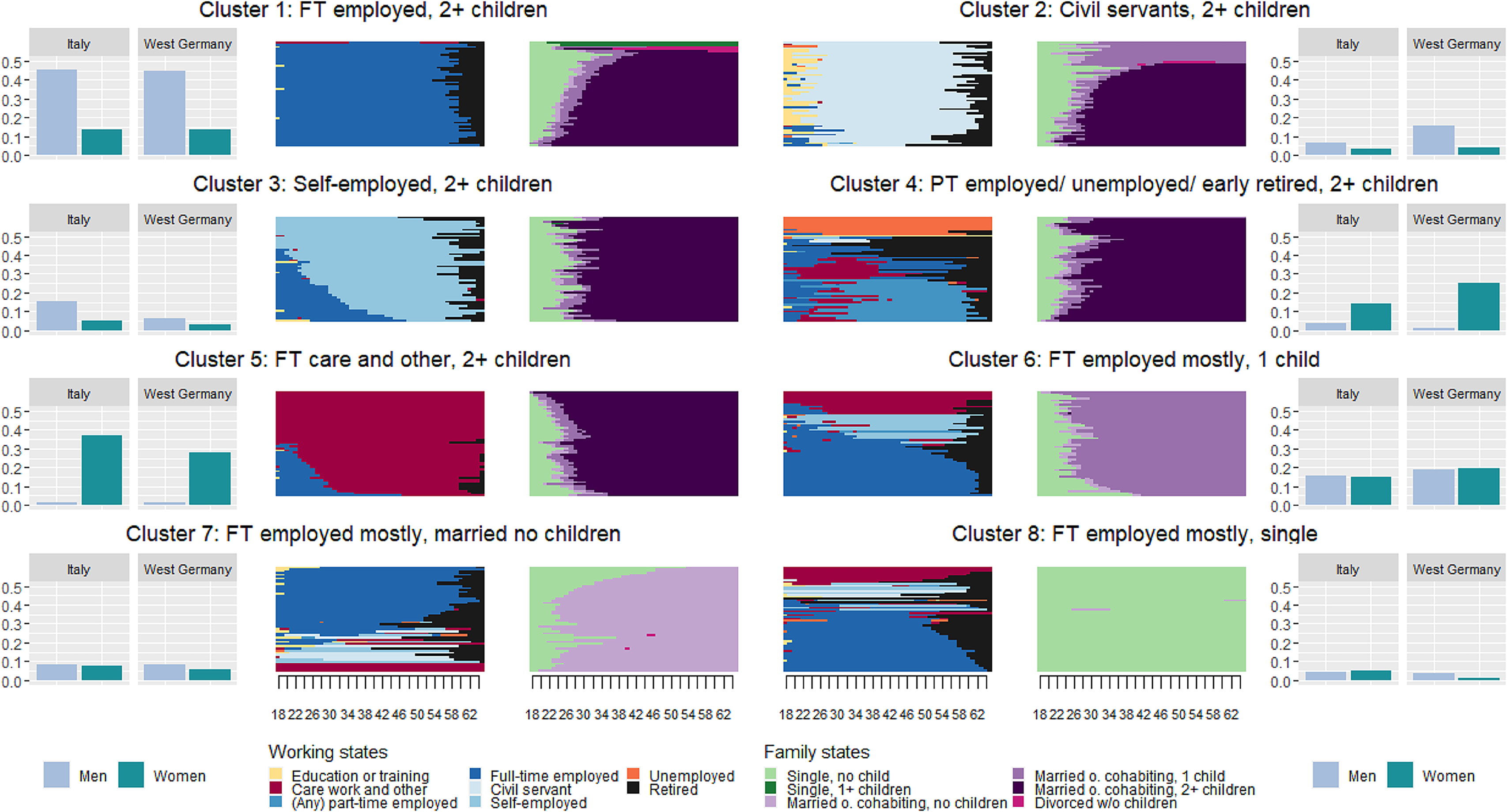
Work and family life courses: relative frequency sequence plots, distribution by gender and across countries. Notes: (i) Gender-specific distribution on clusters depicted as relative shares per gender; (ii) Clusters depicted as relative frequency sequence plot at the center (Fasang and Liao 2014), with depicting representative life courses per cluster from age 18 to 65. The dissimilarity from the medoid for each plot in this figure is displayed in Figure S1 in the Supplementary Materials. Own calculation based on the analysis sample and SHARE waves 2–6, v7.1.0. Not weighted.

Step II: Kitagawa–Oaxaca–Blinder (KOB) Decomposition

In the second step, we applied a KOB decomposition (Blinder 1973; Kitagawa 1955; Oaxaca 1973) ⁹ to each of the two countries separately ¹⁰ to quantify the share of the gap that was explained by gender differences in average characteristics (i.e., the independent variables introduced in the regression models; explained part, compositional, or endowment effect) and the share of the overall gap that was explained by gender-specific differences in returns to these characteristics, that is, differences in the coefficients (returns or group effect; Kunze 2018). ¹¹ For a general introduction to KOB decomposition, see Jann (2008) and Fortin, Lemieux, and Firpo (2011). In this section, we will first present our application and then justify the analytical decisions by systematically comparing them with alternatives, especially with regard to the specification of the KOB reference coefficient.

The decomposition was based on separate linear regression models by group, here of men and women. We applied the twofold decomposition (Jann 2008: 455), which is computed as:

$${\overline{y}}_M-{\overline{y}}_W=\underset{\mathrm{Unexplained}}{\underbrace{\underset{\mathrm{Intercept}}{\underbrace{{\alpha }_M-{\alpha }_W}}+\underset{\mathrm{Returns}}{\underbrace{{{\overline{X}}^{\mathrm{\prime }}}_M({\hat{\beta }}_M-{\hat{\beta }}^{*})+{{\overline{X}}^{\mathrm{\prime }}}_W({\hat{\beta }}^{*}-{\hat{\beta }}_W)}}}}+\underset{\mathrm{Explained}}{\underbrace{{({\overline{X}}_M-{\overline{X}}_W)}^{\mathrm{\prime }}{\hat{\beta }}^{*}}}$$

where ${\overline{y}}_M-{\overline{y}}_W$ stands for the average GPG. ${\overline{X}}_M$ and ${\overline{X}}_W$ denote vectors of mean values of the independent variables for men and women. ${\alpha }_M$ and ${\alpha }_W$ denote the intercepts and ${\hat{\beta }}_M$ and ${\hat{\beta }}_W$ the coefficient vectors of men (M) and women (W) from the gender-specific linear regression model. ¹² $\hat{\beta }*$ is a so-called nondiscriminatory or reference coefficient vector. In the two-fold decomposition applied here, the standard assumption is that the reference coefficient, $\hat{\beta }*,$ captures returns that are not subject to discrimination. To achieve this, the “non-discriminatory coefficient vector” (Jann 2008: 455) must be estimated or defined. In our illustrative application, we wanted to apply a pension reward structure that did not discriminate with regard to the groups of interest. The literature suggested different options for defining a nondiscriminatory reward structure in terms of the outcome, here pension income, that we discuss below. Since we were interested in the contribution of each life-course cluster to the gap in outcomes, we focused on the detailed decomposition, which revealed the contribution of each individual predictor, respectively (Jann 2008). The total explained and unexplained shares were thus less relevant for our application.

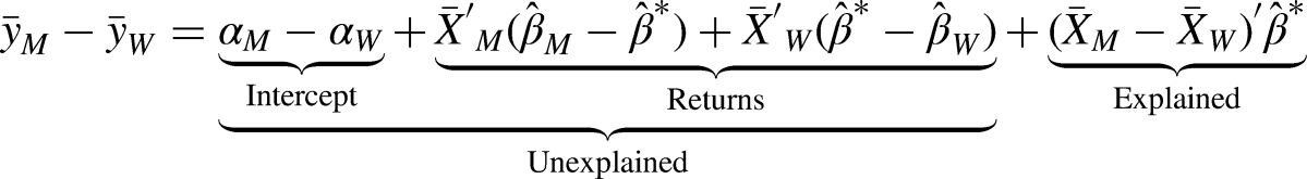
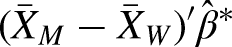
The explained part weighted the mean gender difference in characteristics by the nondiscriminatory coefficient.

$$({\overline{X}}_M-{\overline{X}}_W{)}^{\mathrm{\prime }}{\hat{\beta }}^{*}$$

In combination with SA, the explained shares indicated what part of the gap in the outcome was associated with the group-specific distribution over different trajectory types (row percentages, see Section “Choice of Reference Coefficients”). In our application, the work–family life-course clusters were the main characteristics of interest. The explained part thus quantifies the share of the GPG that was driven by the gender segregation of work–family life-course clusters, that is, men and women experiencing different life courses. Note that such associations should only have appeared if a pension system rewarded typical male and female life-course patterns differently. Even if men and women had completely separate life-course clusters, GPGs could have been very small if the typical male and female life course trajectories yielded similar returns. For example, the explained part indicates what part of the gap was due to the underrepresentation of women in a certain life-course cluster $({\overline{X}}_M-{\overline{X}}_W)$ , such as continuous full-time employment, that is highly rewarded by the pension system (indicated by a high return; $\hat{\beta }*$ ). The interpretation of the explained part that refers to compositional differences is thus sensitive to the underlying reward structure of the outcome.

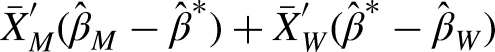
The total unexplained part consists of two components. First, the sum of the group differences in the intercept from the group-specific regression models (intercept component). Second, the sum of the differences between the respective group-specific coefficients from the reference coefficient (here: the male and female coefficients, see Section “Choice of Reference Coefficients”; returns component or effect). Differences in the intercept reflect differences in returns for men and women unrelated to life-course-cluster membership. These emerge due to overall unobserved heterogeneities and within-cluster heterogeneity. Thus, given that the intercept component is mostly comprised of unobserved heterogeneity, we focused on the component of the unexplained share arising from different returns for the same life-course patterns (returns component):

$${\overline{X}}_M^{\mathrm{\prime }}({\hat{\beta }}_M-{\hat{\beta }}^{*})+{\overline{X}}_W^{\mathrm{\prime }}({\hat{\beta }}^{*}-{\hat{\beta }}_W)$$

In combination with SA, the returns component of the unexplained shares indicates to what extent the different groups within the same cluster—that is, with a similar endowment—were rewarded differently in the outcome. Applied to our example, they show what part of the GPG was due to differences in the pension incomes of men and women who experienced the same work–family life-course cluster. In other words, GPGs might have been very high even if life-course clusters were not gender segregated at all but men and women received different pension incomes for the same work–family life-course cluster. ¹³

Three key modeling choices and interpretations in KOB require special attention in combination with SA: (a) the choice of the reference coefficient, (b) dealing with (group-specific) within-cluster heterogeneity and its implications for the interpretation of the returns component, and (c) the specification of the baseline categories for categorical variables (here: clusters).

Choice of Reference Coefficients

One of the most important parameters of KOB decomposition (albeit one that is often not discussed in empirical applications) is the choice of the reference coefficients, as it is consequential for the results (Fortin et al. 2011: 47ff.) and has implications for interpreting the estimates. For the two-fold decomposition, we had to define the nondiscriminatory reference category, which we assumed was not subject to discrimination. There were multiple suggestions for estimating the reference coefficients (Jann 2008; Rahimi and Hashemi Nazari 2021). However, because there is no consensus in the literature and the choice of the reference coefficients also depends on theoretical and empirical considerations, we systematically compared the most prominent options and our proposal of cluster-specific reference coefficients with regard to their general and specific advantages and disadvantages in the SA–KOB combination. Table 1 and Table A4 in the supplemental material give an overview of the benefits and shortcomings of using the different options of reference coefficients as well as their interpretation.

Table 1.

Options for Reference Coefficients.

Reference coefficient option	I.a) Group 1 (here: men)	I.b) Group 2 (here: women)	II) Pooled	III) Cluster-specific majority group
Concept	Regression coefficients from group 1: ${\hat{\beta }}_M$	Regression coefficients from group 2: ${\hat{\beta }}_W$	Regression coefficients from pooled model over both groups: $\hat{\beta }*$	For group-specific clusters: coefficients of the majority group.For group-neutral clusters: coefficients of the theoretically nondiscriminatory group.
Explained part	$({\overline{X}}_M-{\overline{X}}_W{)}^{\mathrm{\prime }}{\hat{\beta }}_M$	$({\overline{X}}_M-{\overline{X}}_W{)}^{\mathrm{\prime }}{\hat{\beta }}_W$	$({\overline{X}}_M-{\overline{X}}_W{)}^{\mathrm{\prime }}\hat{\beta }*$	$({\overline{X}}_M-{\overline{X}}_W{)}^{\mathrm{\prime }}{\hat{\beta }}_M$ or $({\overline{X}}_M-{\overline{X}}_W{)}^{\mathrm{\prime }}{\hat{\beta }}_W$
Returns component from unexplained part	${\overline{X}}_W^{\mathrm{\prime }}({\hat{\beta }}_M-{\hat{\beta }}_W)$	${\overline{X}}_M^{\mathrm{\prime }}({\hat{\beta }}_M-{\hat{\beta }}_W)$	${\overline{X}}_M^{\mathrm{\prime }}({\hat{\beta }}_M-\hat{\beta }*)+{\overline{X}}_W^{\mathrm{\prime }}(\hat{\beta }*-{\hat{\beta }}_W)$	${\overline{X}}_W^{\mathrm{\prime }}({\hat{\beta }}_M-{\hat{\beta }}_W)$ or ${\overline{X}}_M^{\mathrm{\prime }}({\hat{\beta }}_M-{\hat{\beta }}_W)$
Benefits	Straightforward interpretation Reflects assumption that one group is not discriminated against		Sensitive to the group composition of the covariates and implications for the rewarding structure	Straightforward interpretation Sensitive to the group composition of the covariates and implications for the rewarding structure
Limitations	Nondiscrimination assumption unlikely to hold (esp. for all categories of all covariates of interests) Disregards group composition of the cluster		Artificial rewarding structure Unclear which group drives coefficient No straightforward interpretation	Necessary to define thresholds for group-specific and neutral clusters & choice of majority group; application-specific
Specifics for SA-KOB	Concept theoretically and empirically challenged in case of high level of group-specific life-course clusters		In case of highly group-specific life-course cluster, the less typical group might skew the nondiscriminatory coefficients in the pooled regression model	Addresses group-specific life-course clusters and its theoretical and empirical implications Addresses some issues of group-specific within-cluster heterogeneity as majority group more likely to be coherent with overall cluster characteristics

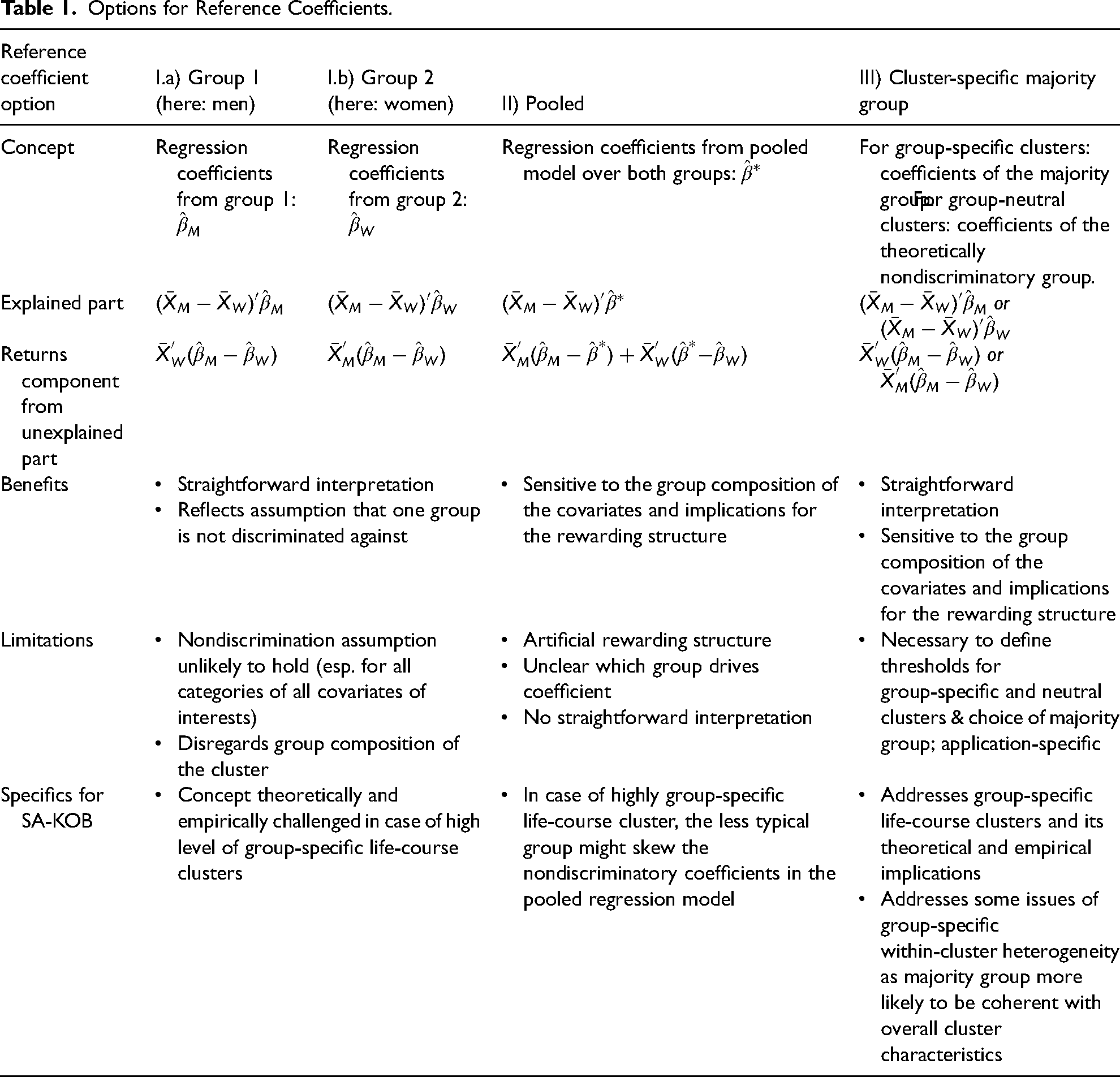
Option I: using the coefficients of one group for all covariates. Discrimination might only be directed toward one of the groups of interests, for example, women; therefore the coefficients of the other group, for example, men, might be a good proxy for a nondiscriminatory rewarding structure. These coefficients are obtained from regression models for the respective group and can then be applied as the reference coefficients for all covariates used in the decomposition. In the gender wage-gap literature, for example, the male coefficients (i.e., coefficients from regression model for men only) are usually used as the reference because it is assumed that wage discrimination is not directed against men (e.g., Blau and Kahn 2017; Kunze 2008). Female disadvantages in pension income are particularly likely because most pension systems, including those of Germany and Italy, are structured around a typical male life course by rewarding stable, full-time employment (see Section “Illustrative Application: Life Courses and Gender Pension Gaps in Germany and Italy”). Thus, in our application, the coefficients of the regression models of men come closest to a nondiscriminatory return for pension income in general terms (see Table A4 in the supplemental material for example interpretations of the KOB estimates). However, this might not apply to all clusters.

When combining KOB and SA, some life-course clusters might contain much higher shares of the group that is not chosen as the reference, in our case, women. This could be problematic for at least two reasons. First, the underrepresented group in that life-course cluster is more likely to deviate from the majority group in some characteristics of the life-course trajectories and the return for this smaller group may be more likely to be biased by outliers. Second, the reward structure (in this case, the pension system) might have some special benefits that only apply to the majority group. For example, many pension systems have specific unpaid care benefits that are (more or less explicitly) directed to typical female life courses dominated by care work. When using the coefficients for men (or the minority group more generally) as reference, such benefits are not reflected in the reward structure used in the decomposition. Furthermore, especially when groups are very unequally distributed across life-course clusters or when within-cluster heterogeneity varies across groups (see discussion of guidelines below), it might be more difficult to choose the reference coefficients for all clusters based on one group than in usual applications of KOB. The researcher will have to decide on which clusters to compromise on, because most likely one group—here, either men or women—will not be the ideal reference for all clusters. Disregarding the group composition of clusters for the choice of references means that researchers will inevitably apply theoretically or empirically inappropriate reference coefficients for some of the clusters.

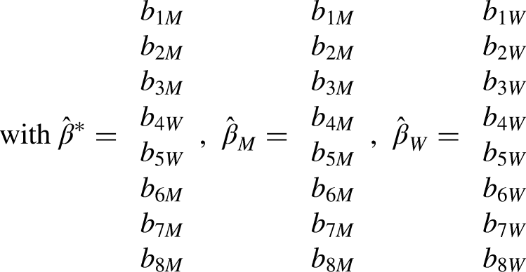
Option II: pooled reference coefficients. Another alternative is to use coefficients from a pooled regression model of both decomposition groups by merging the reward structures of both groups, so that the reward structure considers the group composition of the covariates (Neumark 1988). Even though this is a widely used strategy, it leads to ambiguous interpretations because the reference is an artificial quantification that does not apply to any of the groups in real life (see Table A4 in the supplemental material). As a result, it is unclear what the reward structure actually captures. For example, it is impossible to tell whether the pooled coefficients are driven by one of the groups (especially the majority group) or represent a well-balanced combination of the reward structures of both groups. Additionally, the pooled reference coefficients might be skewed by less typical minority-group life courses in the cluster because they are based on regression models for the whole sample. Related strategies use the weighted average of the male and female coefficients or weight them based on group sizes (Cotton 1988; Reimers 1983). Yet these approaches generally suffer from similarly ambiguous interpretations as pooled reference coefficients.

Option III: cluster-specific reference coefficients using the majority group for each cluster. Addressing the limitations of options I and II, we suggest using cluster-specific reference coefficients based on the group for which the life course is more typical. For example, if a life-course cluster is much more typical for men (i.e., men are the majority group), the male coefficient should be used as the reference for this cluster. But if another life-course cluster is more typical for women, we should use the female coefficient as the reference. We propose this cluster-specific specification of the reference coefficients as a particularly suitable approach when combining SA and KOB.

Compared to using the regression coefficients from one group (option I), our preferred alternative (option III) prevents researchers from using a reference based on a nontypical and small subgroup of a given life-course cluster (and therefore with a probably nontypical reward) as a nondiscriminatory coefficient. An example arises when a few men, who systematically engaged in much less care work compared to the female majority group in a cluster, are assigned to the same cluster characterized by care work. Additionally, gender-oriented policy interventions, such as childcare benefits in pensions, are likely to be picked up by women's reward structures but not by men's. Thus, for such a life-course cluster, it is substantively and theoretically meaningful to use women's reward structures as a reference.

Similarly, compared to using the pooled reference coefficients (option II, Table 1), using cluster-specific references based on the majority group (option III) prevents the reference coefficients from being driven by outliers in the reference group. At the same time, option III is sensitive to the group composition of the covariates and the implications for the reward structure but offers a more straightforward interpretation than using the pooled coefficient.

In most applications, cluster-specific reference coefficients from the majority group (option III) will perform best from the theoretical and empirical point of view. The majority group in the specific life-course cluster is less likely to be discriminated against and the group's returns might be closest to the “real” returns for the cluster. The estimation of the returns for the majority group will be more robust than those obtained by using the other options, because they are less likely to be affected by outliers.

Empirically, the results will tend to be similar to those obtained when using the pooled reference coefficients, because pooled coefficients are likely driven by the majority group in the clusters (confirmed in our illustrative application, see Supplementary Materials E1). But using cluster-specific references (option III) allows for a clearer and more substantively relevant interpretation. Depending on which group is the majority in the cluster, the shares can be interpreted in the same way as they could be when using the coefficients of one group (option I; see interpretation examples in Table A4 in the supplemental material). To sum up, option III combines the benefits of the other two options (straightforward interpretation and consideration of group composition of clusters, see Table 1) while providing researchers with greater flexibility to adjust the reference based on specific empirical cases or theoretical or policy considerations.

Guidelines for Cluster-Specific Reference Coefficients Using the Majority Group

We propose a set of guidelines for the application of cluster-specific reference coefficients (option III). To begin with, researchers must identify group-specific life course clusters and the majority groups. For this, we suggest applying (a) theoretical, (b) empirical, and (c) statistical considerations. First, theoretically, one has to consider whether the reward structure of a given cluster contains group-specific benefits that are expected to be exclusive to a particular group's reward structure (e.g., pension benefits for care work will mostly be picked up in women's reward structures). If this is the case, there might be reasons to pick this group as the reference. Second, when seeking to identify the majority groups empirically, researchers can use a descriptive table that shows the interaction between groups and clusters (see Table 2).

Table 2.

Cross Table of Gender with the Clusters (Illustrative Application, For Italy).

(a) row %
	Cluster 1	Cluster 2	Cluster 3	Cluster 4	Cluster 5	Cluster 6	Cluster 7	Cluster 8	Total
Men	45.39	6.48	15.4	3.61	1.18	15.48	8.25	4.2	100
Women	13.78	3.25	4.97	13.78	36.85	14.84	7.42	5.1	100
Mean	28.75	4.78	9.91	8.97	19.96	15.14	7.82	4.68	100
Abs. Difference Men/Women	31.61	3.23	10.43	10.17	35.67	0.64	0.83	0.9
Rel. Difference Men/Women	69.64	49.85	67.73	73.8	96.8	4.13	10.06	21.43

(b) column %
	Cluster 1	Cluster 2	Cluster 3	Cluster 4	Cluster 5	Cluster 6	Cluster 7	Cluster 8	Mean
Men	74.76	64.23	73.59	19.07	2.8	48.39	50	42.54	47.35
Women	25.24	35.77	26.41	80.93	97.2	51.61	50	57.46	52.65
Total	100	100	100	100	100	100	100	100	100
Abs. Difference Men/Women	49.52	28.46	47.18	61.86	94.4	3.22	0	14.92
Rel. Difference Men/Women	66.24	44.31	64.11	76.44	97.12	6.65	0	35.07

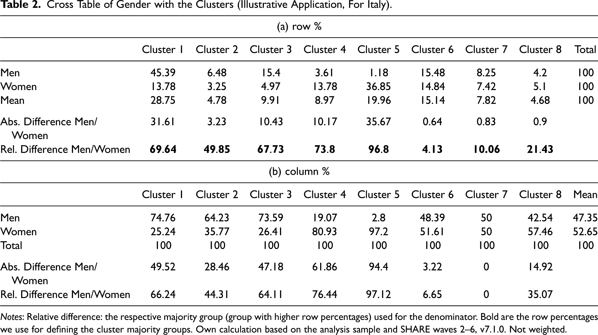
Notes: Relative difference: the respective majority group (group with higher row percentages) used for the denominator. Bold are the row percentages we use for defining the cluster majority groups. Own calculation based on the analysis sample and SHARE waves 2–6, v7.1.0. Not weighted.

Both column and row percentages can be considered. ¹⁴ However, the column percentages are sensitive to the group sizes. Since, unlike the fairly equal distribution of men and women in our application, group sizes may differ, we suggest considering the gender gap in the distribution over the clusters, that is, in the row percentages, which are equivalent to the ${\overline{X}}_A$ and ${\overline{X}}_B$ used in the decomposition. We categorized life-course clusters as group-specific if the relative gender gap in the distribution was greater than 50% ( $50<100*(({\overline{X}}_A-{\overline{X}}_B)/{\overline{X}}_A)$ , with ${\overline{X}}_A>{\overline{X}}_B$ ). The choice of the cut-off for defining majority groups depended on the overall level of the group distribution on clusters. For example, in scenarios with lower levels of group-specific segregation of life courses, researchers might choose thresholds of 30% or 40%. Furthermore, comparing the cluster characteristics across groups can help identify the group that shares the key characteristics of the cluster and thus guide the choice of the majority group (i.e., men or women in our illustration). Lastly, the categorization of the majority group can be statistically validated by comparing the ASW by group for each cluster. The ASW—that is, the average fit of the trajectories to the cluster—should be higher for the majority group. ¹⁵

In a second step, the researcher must decide which reference to use for group-neutral clusters, that is, life-course types with no clear majority group. For group-neutral life-course clusters, we suggest using the reference coefficients of the overall nondiscriminatory group. This should be guided by theoretical assumptions on which group is least discriminated against regarding the outcome of interest. For wages and pensions, for example, researchers typically expect that men are not discriminated against, suggesting the coefficients of the regression model for men should be used as the reference for gender-neutral clusters.

In our application, we illustrate the choice of cluster-specific references (option III) based on the outcome of the SA at the beginning of Section “Gendered Work–Family Life Courses.” For our main model, we specify cluster-specific reference coefficients based on the coefficients from the linear regression models for women for the female majority work–family life courses ( $b_{4W},b_{5W}$ ); we specify cluster-specific reference coefficients based on men's coefficients for the male majority and gender-neutral clusters ( $b_{1M},b_{2M,}{b}_{3M},b_{6M,}{b}_{7M},b_{8M}$ ):

$${\overline{y}}_M-{\overline{y}}_W=({\overline{X}}_M-{\overline{X}}_W{)}^{\mathrm{\prime }}{\hat{\beta }}^{*}+{\overline{X}}_M^{\mathrm{\prime }}({\hat{\beta }}_M-{\hat{\beta }}^{*})+{\overline{X}}_W^{\mathrm{\prime }}({\hat{\beta }}^{*}-{\hat{\beta }}_W)$$

$$\mathrm{with}{\hat{\beta }}^{*}=\begin{array}{c}\begin{array}{c}\begin{array}{c}{b}_{1M}\\ b_{2M}\\ b_{3M}\end{array}\\ b_{4W}\\ b_{5W}\end{array}\\ b_{6M}\\ \begin{array}{c}{b}_{7M}\\ b_{8M}\end{array}\end{array},{\hat{\beta }}_M=\begin{array}{c}\begin{array}{c}\begin{array}{c}{b}_{1M}\\ b_{2M}\\ b_{3M}\end{array}\\ b_{4M}\\ b_{5M}\end{array}\\ b_{6M}\\ \begin{array}{c}{b}_{7M}\\ b_{8M}\end{array}\end{array},{\hat{\beta }}_W=\begin{array}{c}\begin{array}{c}\begin{array}{c}{b}_{1W}\\ b_{2W}\\ b_{3W}\end{array}\\ b_{4W}\\ b_{5W}\end{array}\\ b_{6W}\\ \begin{array}{c}{b}_{7W}\\ b_{8W}\end{array}\end{array}$$

We apply the different options for setting the reference coefficients to our empirical case and discuss the results in Supplementary Materials E1. Our main findings are robust when applying all discussed options and we illustrate how, in addition to being easier to interpret, option III has advantages in our case based on theoretical and empirical considerations.

In the case of highly group-specific covariates, researchers might want to apply our suggested option to standard KOB applications as well and choose the reference coefficients for each of the covariates or categories separately.

(Group-Specific) Within-Cluster Heterogeneity

Poorly classified cases in the cluster typology, or outlier life courses that do not clearly fit into any cluster might also affect reference coefficients. These life courses are not a good match to the main characteristics of the life-course type. This is a common issue, as cluster analysis will always allocate each case to a cluster (see Raab and Struffolino 2022). What this means for SA–KOB is that the reference coefficients used to weight the mean differences between the groups when computing the explained share might not be representative and fail to reflect the nondiscriminatory returns for the life-course cluster if it is skewed by poorly assigned individuals instead. The explained part of the KOB might thus be overestimated or underestimated.

Within-cluster heterogeneity might affect the returns component of the unexplained part of the decomposition as well and especially so if the within-cluster heterogeneity is group specific. The group differences within clusters means that there are some differences between groups with regard to their trajectories, here men and women, in endowment with the same characteristic, here work–family life-course cluster. If this is the case, the groups within the same cluster have similar life courses but not the very same ones—these are understood as different empirical realizations of a similar underlying life-course type. However, as the main idea of the returns component in the KOB is to show how the returns to the same characteristics (e.g., tertiary education) differ by groups by holding the endowment with this characteristic constant, this interpretation cannot be applied to characteristics that are highly heterogeneously endowed. As a result, the differences in returns by group might be driven by the group-specific heterogeneity within the same life-course clusters.

When combining SA and KOB, the returns component will likely never show the impact of different returns to the same endowment but rather to a similar trajectory or the same life-course cluster. That is, the returns component does not necessarily distinctly show how the different groups with the exact same life course are rewarded differently as intended in the standard KOB decomposition but could also pick up ways that the groups are rewarded differently because of differences within the same life-course cluster. Researchers should keep this in mind when interpreting the returns component in SA–KOB applications and generally only use sufficiently coherent cluster typologies to ensure meaningful results in SA–KOB.

More generally, within-cluster heterogeneity underlines the complexity of life courses and highlights an additional dimension of inequality. ¹⁶ As such, some within-cluster differences might only become visible through SA and can be accommodated in the modeling and interpretation (Aisenbrey and Fasang 2010); for instance, the sum of the years in a specific state used previously in decomposition analyses might conceal differences in the volatility, timing, or order of these states between groups. Such group-specific heterogeneity is not necessarily specific to the SA–KOB combination but might apply to any variable used for KOB, albeit it may be less visible. For instance, a common assumption in KOB would be that women and men with tertiary education have, overall, the same endowment of education. However, heterogeneity within tertiary education is plausible due to differences in the educational trajectory that leads to a certain degree, different fields of study, or different reputations of the university among individuals, which are likely to influence wage and pension returns. By including more (life-course-related) variables simultaneously than in previous decomposition techniques (e.g., differentiating between full-time and part-time employment, civil service, and self-employment) and considering the timing and order of these along life courses, the SA–KOB combination can reduce heterogeneity within categories. At the same time, visualization techniques make heterogeneity explicit and can inform the interpretation of the results.

SA provides tools to deal with within-cluster heterogeneity by identifying individuals who are poorly allocated to the clusters based on low silhouette widths and excluding them from further regression-based analyses (Jalovaara and Fasang 2020). Estimating the KOB when excluding poorly classified sequences in the cluster typology shows how sensitive the results are to (group-specific) within-cluster heterogeneity: see Supplementary Materials E4 for a discussion of this sensitivity check. We recommend assessing the impact of within-cluster heterogeneity on the KOB results. When using relative cut-offs for silhouette widths sensitive to the cluster-specific silhouette distribution, we found that the returns component in our illustrative application remained roughly the same, while the explained shares tended to be larger (Table S4.2 in the Supplementary Materials). This is in line with the generally stronger effect sizes for sequence clusters in regression-based analyses when poorly classified cases are excluded and only individuals above a certain silhouette threshold are retained to ensure relatively “pure” types in the life-course clusters (Jalovaara and Fasang 2020).

Baseline Categories of Categorical Variables and Choice of Controls

The decomposition results for categorical variables, including life-course clusters, differ depending on the baseline category used (Fortin et al. 2011; Jann 2008). We normalized the categorical variables to calculate shares of the GPG arising from the returns component that were independent of the choice of the reference category: The coefficients in the OLS models underlying the KOB indicate deviations from the grand mean and not from the chosen reference category (Jann 2008; Yun 2005). Normalization is helpful when combining decomposition tools with SA. Especially in empirical scenarios of highly group-specific life-course clusters, it is more difficult to find a theoretically meaningful and empirically unproblematic baseline category for all groups than in standard applications of KOB. While researchers have to choose the same baseline category for all groups for KOB, the standard life course, which would be a suitable baseline category, will likely differ across groups if life courses are group specific. Adding more dimensions, such as country comparisons, will add more difficulties, since standard life courses are also likely to differ across countries.

A related issue is which control variables to include in addition to life-course clusters. To avoid multicollinearity issues and over controlling, additional control variables should generally be temporally located prior to the start of the life-course sequences, they should not be components of the life-course sequences, and they should be largely unrelated to them. For example, researchers are not advised to control for education when it is a sequence state, but variables such as parental education or region are unproblematic. Accordingly, we only adjusted the main models for birth cohort and survey wave but undertook robustness checks with more extensive control scenarios as presented in Supplementary Materials E5.

Further Robustness Checks

Besides systematically comparing alternatives with regard to (a) the choice of reference coefficients and dealing with (b) within-cluster heterogeneity, we conducted a series of further robustness checks. We showed that the main association between the GPG and the life-course clusters was not driven by: (i) differences in education or migration background between men and women (Supplementary Materials E5, Table S4.3) or (ii) the use of weights (Supplementary Materials E6, Table S4.4). Furthermore, we discuss our approach to dealing with the common support problem that might occur when life-course clusters from the first step of the SA–KOB decomposition are highly group-specific (Supplementary Materials E6).

Software and Packages

We performed SA in R using the packages TraMineR, TraMineRextras (Gabadinho et al. 2011), and WeightedCluster (Studer 2013) and used the oaxaca package (Jann 2008) for decomposition in STATA. However, both SA and KOB can be performed in R and STATA. In STATA, the packages for sequence analysis are SQ (Brzinsky-Fay, Kohler, and Luniak 2006) and SADI (Halpin 2017), and in R, oaxaca (Hlavac 2014) can be used for KOB decomposition.

Results of the Illustrative Application on GPGs in Germany and Italy

In this section, we summarize the results of our application to illustrate the potential of SA–KOB to provide new insights into long-standing questions in life-course research, social demography, and stratification. For this, we first replicate the standard KOB approach with our data and briefly discuss the results (Section “Standard KOB Using Life Course Summary Measures”). We then present the results of the MSA (Section “Gendered Work–Family Life Courses”) and of the SA–KOB (Section “SA–KOB Decomposition of Gender Pension Gaps”). In Section “Comparison of SA–KOB With Standard KOB Using Life Course Summary Measures” we compare the results, the benefits, and the limitations of the standard KOB to the SA–KOB decomposition.

Standard KOB Using Life Course Summary Measures

To highlight the theoretical, empirical, and methodological contribution of SA–KOB decomposition compared to the standard decomposition approach in the literature, we replicated KOB decomposition using summary indicators as proxies for family and work life courses (hereafter referred to as “standard model”). For comparability, we used the same life-course states as in the SA but could not include all of them due to high multicollinearity levels. As a result, we opted to include the life-course states that are used most often as main covariates in standard decomposition applications to estimate the GPG (see Table A1) and therefore excluded the duration of care work, retirement, self-employment, years spent in marriage and having one child, and years spent in single parenthood. Please refer to Section E2 of the Supplementary Materials for more details on the multicollinearity issue and on the results; the latter are only summarized briefly in the following paragraphs.

We decomposed the GPG, which amounts to 53% in Italy (€6,651 in absolute terms) and 62% in West Germany (€13,089 in absolute terms). ¹⁷ For the KOB decomposition, we applied the same parameters as in our main analysis to ensure comparability. Table 3 shows the decomposition results. Consistent with previous literature, we found that the lower number of years women spent on average in full-time work compared to men (see Figure S6.1) was the main reason for the GPG in both countries (explained share). Women's pension would increase by €1,368 in Italy (21% of GPG) and €3,136 in West Germany (24% of the GPG) if they worked the same number of years on average as men in full-time employment. The “missing” years women spent working in the civil service are another driver of the GPG but to a much higher extent in West Germany than in Italy (15% vs 1% of the GPG). While the higher number of years spent on average in education by men after age 17 explains 7% of the GPG in West Germany, 5% of the GPG in Italy is due to the greater number of years on average women have spent in unemployment. In both countries, the gender inequality in pensions would be even higher if women spent as few years as men in part-time employment (1% of GPG in Italy, and 10% in West Germany). We find that family life characteristics matter as well but to a lesser extent. In both countries, the GPG would be even larger if women were childless and single for as many years as men (see Figure S6.2), and in Italy a part of the GPG is due to the greater number of years women spent married and with two or more children.

Table 3.

Results from Standard KOB Decompositions.

	Italy				West Germany
Mean pension inc. men	12,660**				21,119**
	(64.22)				−58.62
Mean pension inc. women	6,009**				8,030**
	(28.42)				−26.82
Absolute GPG	6,651**				13,089**
	(21.27)				−26.33
Explained, total	1,682**				4,499**
	(6.781)				−6.457
Unexplained, total	4,970**				8,590**
	(12.09)				−12.55

	explained	shares	returns	shares	explained	shares	returns	shares
Years FT employment	1,368**	20.56%	−706.7**	−10.63%	3,136**	23.96%	206.7	1.58%
	(6.491)		(−3.644)		−5.452		−0.431
Years PT employment	−68.74**	−1.03%	−116.2**	−1.75%	−1,282**	−9.79%	−34.23	−0.26%
	(−2.964)		(−3.268)		(−6.136)		(−0.973)
Years civil service	79.66*	1.20%	−311.1**	−4.68%	1,939**	14.82%	−134.9	−1.03%
	(2.224)		(−4.926)		−8.523		(−1.340)
Years education	109.7	1.65%	629.9**	9.47%	940.9**	7.19%	916.5**	7.00%
	(1.141)		(3.931)		−3.169		−2.879
Years unemployment	322.6**	4.85%	−362.1*	−5.44%	156.3	1.19%	−280.2	−2.14%
	(2.798)		(−2.450)		−0.843		(−1.066)
Years divorced	3.471	0.05%	30.66	0.46%	27.32	0.21%	−514.3**	−3.93%
	(0.299)		(1.078)		−0.621		(−3.764)
Years married, 2 + ch.	145.3**	2.19%	−776.8	−11.68%	55.69	0.43%	517.6	3.95%
	(2.782)		(−1.324)		−0.51		−0.541
Years married, no children	−1.068	−0.02%	−60.36	−0.91%	44.46	0.34%	87.09	0.67%
	(−0.0634)		(−0.423)		−1.226		−0.386
Years single, no children	−254.3**	−3.82%	−856.5**	−12.88%	−558.2**	−4.26%	−829.2**	−6.33%
	(−3.080)		(−3.685)		(−3.278)		(−2.840)
Constant			7,648**				8,369**
			(6.353)				−4.163
n male	1357		1357		804		804
n female	1509		1509		815		815

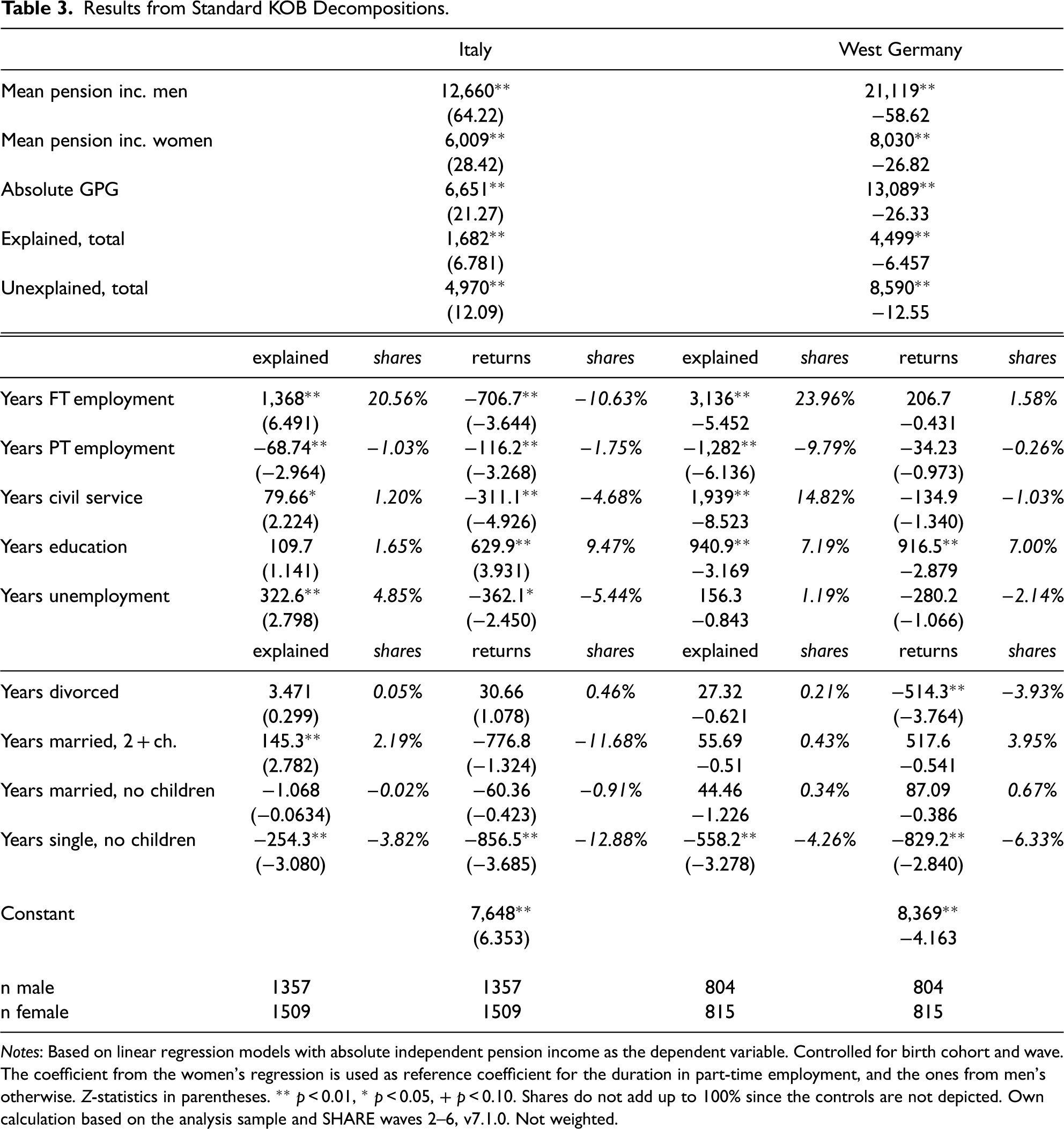
Notes: Based on linear regression models with absolute independent pension income as the dependent variable. Controlled for birth cohort and wave. The coefficient from the women's regression is used as reference coefficient for the duration in part-time employment, and the ones from men's otherwise. Z-statistics in parentheses. ** p < 0.01, * p < 0.05, + p < 0.10. Shares do not add up to 100% since the controls are not depicted. Own calculation based on the analysis sample and SHARE waves 2–6, v7.1.0. Not weighted.

The returns component reveals that substantial parts of the gap in both countries are due to lower pension returns for women compared to men for years spent in education. In Italy, the GPG would be even higher if women received the same returns for full-time employment and unemployment as men. In West Germany, in contrast, the GPG would be even higher if women received the same pension returns for years spent being divorced as men.

As suggested by previous decomposition literature (Table A1), the present analysis's main conclusion based on the standard KOB is thus that women have much lower pensions than men due to their fewer years spent in employment.

Gendered Work–Family Life Courses

Figure 1 depicts the eight work–family life-course clusters, with the work life courses on the left and the family life courses at the right-hand side. The outer portions of the figure show the gender distribution over these clusters by country.

In line with expectations, the work–family life-course profiles in the clusters mirror the traditional distribution of paid and unpaid work between men and women as incentivized by the conservative and family-oriented institutional and normative contexts in both welfare states in the second half of the twentieth century.

Cluster 1 reflects a prototypical male breadwinner life course of early continuous full-time employment in the private sector. Most individuals in this group entered marriage and parenthood between the ages of 20 and 30. It is the most prevalent life-course type (29%). 45% of Italian and West German men experienced this life-course type, compared to only 14% of women (see Table A6), pointing to notable similarities in the unequal gender distribution for this life-course type across countries.

Cluster 2 displays a similar prototypical male breadwinner life course with continuous careers as civil servants after longer periods of education and correspondingly a somewhat later onset of family formation compared to cluster 1. A greater proportion of people in this group have only one child. This pattern is not quite as gendered as the private sector male breadwinner life course, but it is still more exclusively experienced by men, particularly in Germany.

Cluster 3 shows employment lives that transition into self-employment, mostly from full-time private sector work by age 40 and then remain in stable self-employment. Family lives are characterized by having two or more children in stable relationships with a slightly later onset on average compared to clusters 1 and 2. In both countries, this cluster is more common among men than women, especially in Italy.

Together, cluster 1-3 thus distinctly signify typical male breadwinner life courses. This provides empirical support for a strong gender segregation in life courses in the gender-conservative environments, as also found by Madero-Cabib and Fasang (2016).

A tight linkage between work and family life only becomes visible for clusters 4 and 5: changes in working life (mostly from full-time employment to part-time or care work) often parallel family transitions. Both clusters are characterized by early family formation, being married, and having at least two children and are highly dominated by women. For the life courses in clusters 4 and 5, with transitions between employment and care work, the start of the full-time care period corresponds almost exactly to a shift from being single to being married or childbirth, highlighting the interdependence of women's family and working lives.

Cluster 4 is characterized by the absence of stable and paid full-time work. A considerable proportion of respondents have retired early after a short period of full-time employment or are continuously unemployed. Most individuals experience volatile work trajectories, transitioning from full-time employment to longer periods of care work and finally to fairly continuous part-time employment, and to a lesser extent full-time employment, after mid-life. Among West German women, 25% used (interrupted) part-time work to reconcile work and family life; the figure was only 14% in Italy.

Cluster 5 is characterized by care work throughout the whole life course or stable care work after a short period of full-time employment in early adulthood. Care-dominated life courses are most prevalent for women in both countries: they apply to 37% of women in Italy and 28% of women in Germany.

Life-course clusters 6–8 show very similar work lives but different family life courses and are gender-neutral. All three are dominated by continuous full-time employment but contain a substantial share of individuals with continuous care work or self-employment as well. Cluster 6 comprises individuals who are married and have one child. Cluster 7 is characterized by childlessness and relatively late marriages and cluster 8 is characterized by lifelong singlehood.

The highly gender-specific clusters raise challenges for the KOB decomposition in the second step of our analysis, given that there are almost no men in clusters 4 and 5. This empirical finding is specific to our illustrative application and does not appear for SA–KOB more generally. We discuss this issue and a way of dealing with it in detail in Supplementary Materials E6. To reduce the potential impact of lacking common support for men in the female majority clusters 4 and 5, we identified male life courses that are similar to the characteristics of these clusters based on the fit with the cluster (ASW) and life course summary measures. We then reassigned these male trajectories to cluster 4 and 5 for the decomposition to create counterfactuals of men for these highly women-majority clusters manually.

SA–KOB Decomposition of Gender Pension Gaps

We used the MSA cluster typology to decompose the GPG in Italy and West Germany.

For clusters 4 and 5, we used the coefficients from the regression model for women as reference coefficients in the KOB; for all other clusters we use the coefficients for men. First, based on empirical considerations, the share of women more than doubles that of men's for clusters 4 and 5 (relative difference higher than 50%, see Table A6). Comparing the cluster characteristics across groups confirms that women's characteristics are much more in line with the overall cluster characteristics than men's (see Tables A5.1 and A5.2 in the supplemental material). Second, based on theoretical considerations, we prefer to use the women's coefficients as a reference for clusters 4 and 5, as these are more likely to capture pension-related benefits that reward care work and part-time employment, which are more common for women in these clusters. Lastly, the group-specific ASW by cluster and gender validates using women's coefficients as references for cluster 4 and 5: women's life courses are on average a better fit to both clusters (see Figure A1 in the supplemental material).

For similar reasons, we use men's coefficients as references for clusters 1–3. The clusters are more common among men, and men's life courses in these groups mirror the cluster characteristics. Men's coefficients best capture the nondiscriminatory reward structure, given that most pension systems are “shaped around an idealized male worker“ (Grady 2015: 454). This is also why we use men's coefficients for the gender-neutral clusters 6–8, which are characterized by full-time employment careers too. Moreover, men's life courses share the overall working life-course characteristics of these clusters (see Tables A5.1 and A5.2 and detailed discussion in Supplementary Materials E1).

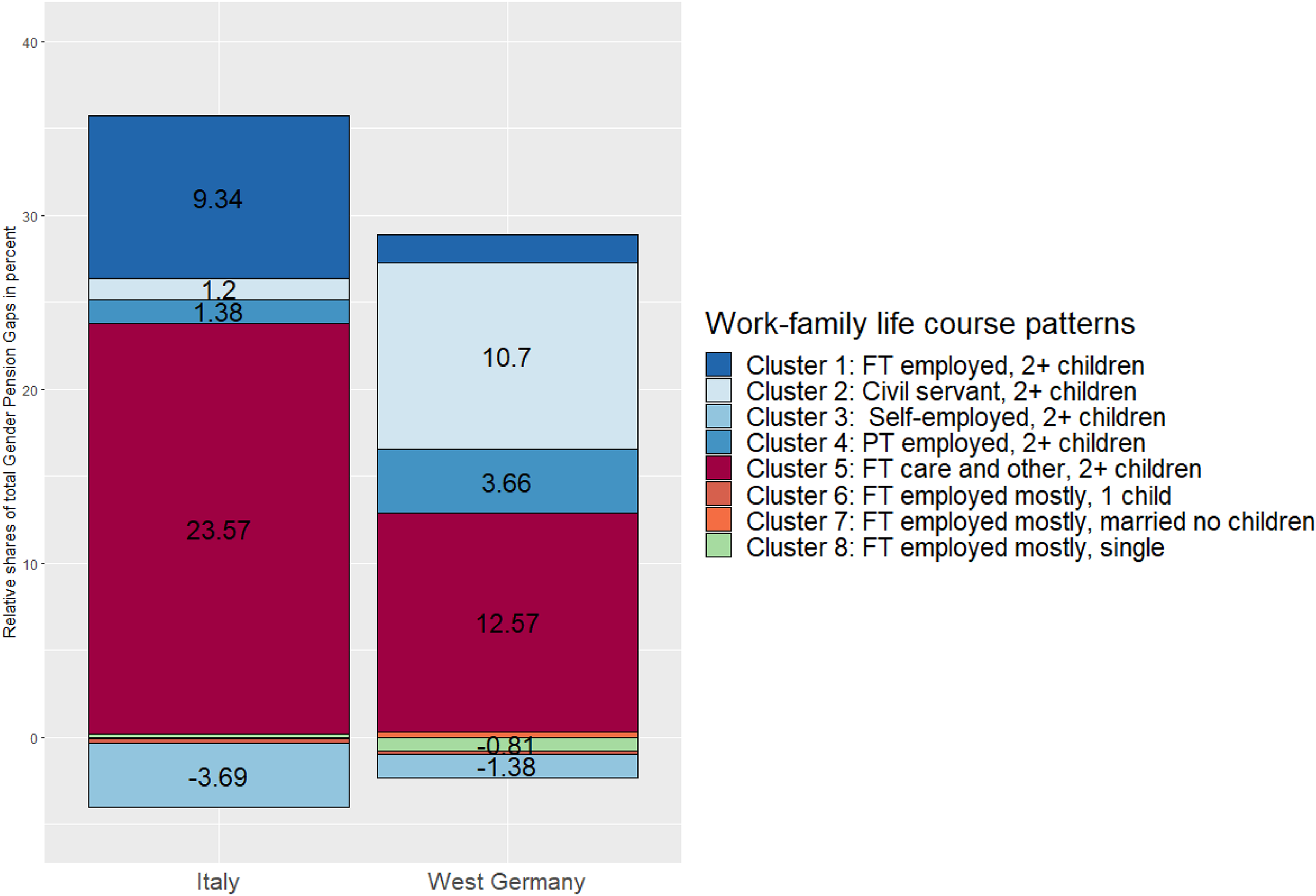
In line with our expectations of relatively large compositional life-course effects on GPGs in both countries, Table 4 shows that 32% of the GPG in Italy and 27% in Germany is explained by the gender-segregation of work–family life courses, that is, men and women experiencing different life courses. ¹⁸ Further, in line with expectations, both compositional and returns effects account for a larger share of GPGs in Italy than in Germany, albeit the country differences in the returns component are relatively small.

Table 4.

Results From SA–KOB Decompositions.

	Italy				West Germany
Mean pension inc. Men	12,660**				21,119**
	−57.31				−53.62
Mean pension inc. Women	6,009**				8,030**
	−37.13				−28.52
Absolute GPG	6,651**				13,089**
	−24.29				−27.03
Explained, total	2,054**				3,514**
	−10.07				−8.725
Unexplained, total	4,597**				9,575**
	−14.52				−17.65

	explained	shares	returns	shares	explained	shares	returns	shares
Sum life courses	2106.281	31.67%	386.66	5.81%	3476.08	26.56%	555.203	4.24%
1 FT employed, 2 + chi.	621.2**	9.34%	92.16	1.39%	214.9	1.64%	99.19	0.76%
	−4.88		−1.178		−1.04		−0.741
2 Civil servant, 2 + chi.	79.72*	1.20%	−84.40*	−1.27%	1,401**	10.70%	2.913	0.02%
	−2.49		(−2.258)		−6.738		−0.0499
3 Self-employed, 2 + chi.	−245.2**	−3.69%	−69.06+	−1.04%	−181.2*	−1.38%	−33.92	−0.26%
	(−3.929)		(−1.655)		(−2.499)		(−0.598)
4 PT employed, 2 + chi.	92.08**	1.38%	−15.25	−0.23%	479.3**	3.66%	−58.72	−0.45%
	−3.069		(−0.247)		−3.784		(−0.791)
5 FT care/other, 2 + chi.	1,568**	23.58%	58.67+	0.88%	1,646**	12.58%	88.07	0.67%
	−13.68		−1.778		−9.03		−1.625
6 FT empl./care, 1 child	−19.3	−0.29%	477.6**	7.18%	−19.99	−0.15%	518.0*	3.96%
	(−0.633)		−4.48		(−0.735)		−2.394
7 FT employed, married	−4.059	−0.06%	87.04	1.31%	41.67	0.32%	−2.24	−0.02%
	(−0.463)		−1.275		−1.134		(−0.0251)
8 FT employed, single	13.84	0.21%	−160.1**	−2.41%	−105.6*	−0.81%	−58.09	−0.44%
	−0.936		(−2.677)		(−2.020)		(−1.574)
n men	1357		1357		804		804
n women	1509		1509		815		815

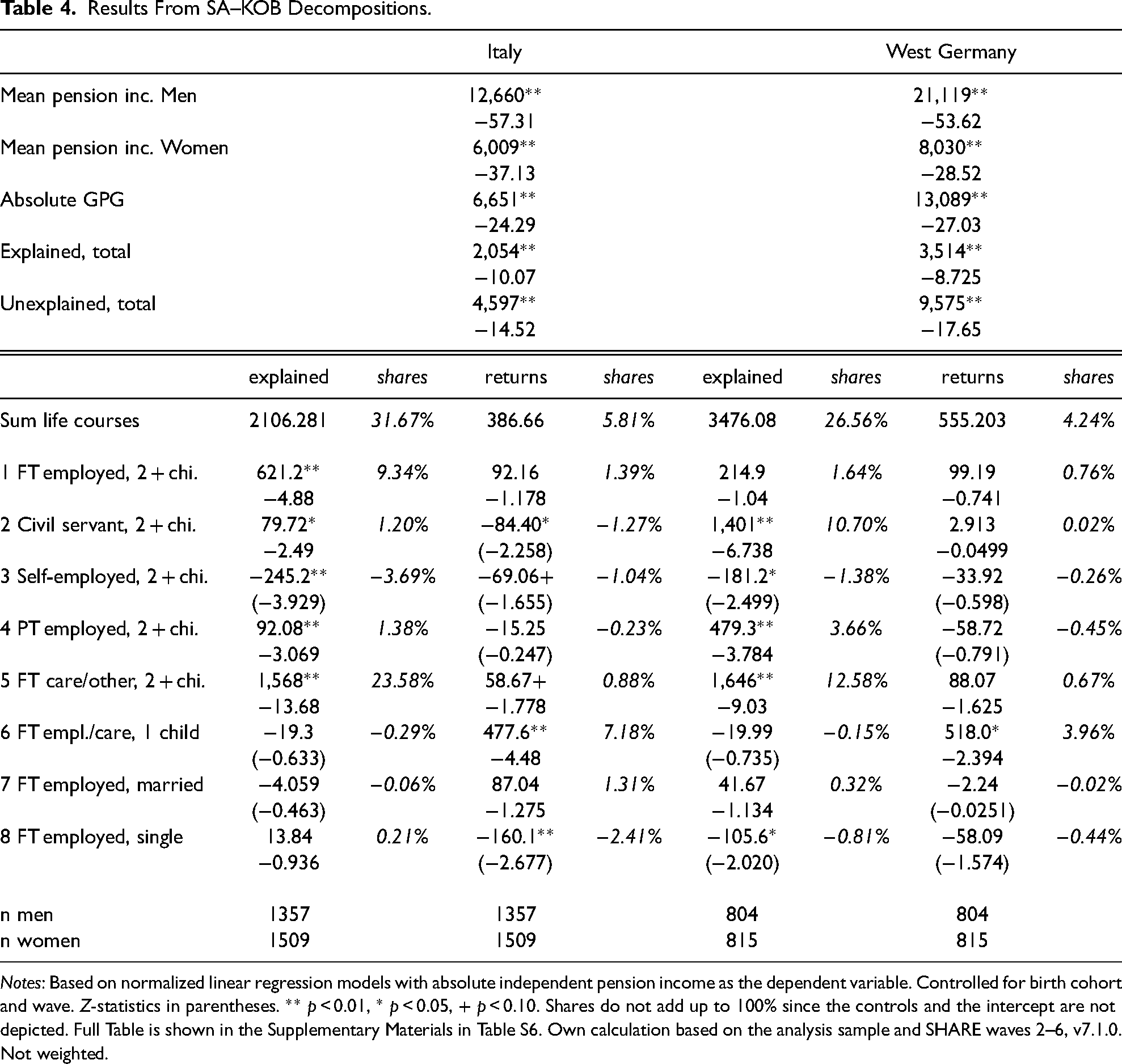
Notes: Based on normalized linear regression models with absolute independent pension income as the dependent variable. Controlled for birth cohort and wave. Z-statistics in parentheses. ** p < 0.01, * p < 0.05, + p < 0.10. Shares do not add up to 100% since the controls and the intercept are not depicted. Full Table is shown in the Supplementary Materials in Table S6. Own calculation based on the analysis sample and SHARE waves 2–6, v7.1.0. Not weighted.

In both countries, the majority female life-course cluster characterized by continuous unpaid care work (cluster 5) is the main driver of the GPG. 24% (€1,568) of the gap in Italy and 13% (€1,646) of the gap in West Germany are due to the absence of almost any men with life courses that are poorly rewarded in the pension system (Tables 3 and 4). The much higher minimum contribution years in Italy means more Italian women with this life course have no pension income (56% of women compared to 23% of men in the cluster, Table A5.1)—less than half of the women in this life course reach the required 20 years of paid work. In Germany, lower qualification criteria give women with employment periods before family formation access to independent pension income (14% of German women in this cluster are without pension income). While both countries provide benefits for an equivalent to a maximum of 1 year per child, women with these life courses are usually engaged in unpaid care work for much longer periods—on average 38 years and 42 years in West Germany and Italy, respectively.

The gender segregation on cluster 4, which is characterized by volatile working life courses, is more strongly associated with the GPG in West Germany than in Italy. The overrepresentation of women in this cluster was responsible for 3.7% of the gap in West Germany and 1.4% of the gap in Italy (Figure 2). Compared to continuous full-time care work (cluster 5), combining care responsibilities with paid part-time employment, periods of unemployment, or early retirement reduces the pension-income penalty for mothers in both countries (returns for cluster 4 and 5, Table 5). But, at the same time, it cannot make up for the lack of full-time employment. Thus, the overrepresentation of women in these two life-course clusters, which are characterized by strong interdependence between work and family lives, would not lead to the large GPG in both countries if their female-typical biographies were rewarded equally to male-typical ones.

Figure 2.

Decomposition results – explained shares by work–family life courses and country. Notes: Percent of shares only displayed if minimum significance level of 10%. Results from KOB decompositions from Table 4. Based on normalized linear regression models with absolute independent pension income as dependent variable. Adjusted for birth cohort und wave. Confidence intervals depicted in Figures S5.1 and S5.2 in the Supplementary Materials. Own calculation based on the analysis sample and SHARE waves 2–6, v7.1.0. Not weighted.

Table 5.

Baseline Coefficients From Linear Regression Analysis Used for SA–KOB, Normalized.

	Italy			West Germany
	Men	Women	Pooled	Men	Women	Pooled
1 FT employed, 2 + children	2061.3	1392.7	1885.9	724.6	−10.36	682.0
2 Civil servant, 2 + children	2778.3	5377.5	3829.7	12454.1	12379.9	12597.4
3 Self-employed, 2 + children	−2473.1	−1083.6	−2112.1	−5532.7	−4426.9	−4968.2
4 PT employed, 2 + children	−1642.4	−1435.4	−1230.6	−3643.4	−2332.1	−1925.9
5 FT care and other, 2 + children	−2299.9	−4574.7	−3997.7	−2668.5	−6395.3	−5542.1
6 FT employed or care, 1 child	2289.7	−927.5	730.9	1160.0	−1495.2	34.79
7 Ft employed, married, no children	819.8	−353.0	396.9	2459.4	2499.1	2686.3
8 Ft employed, single	−1533.6	1604.1	496.9	−4953.5	−219.1	−3564.3

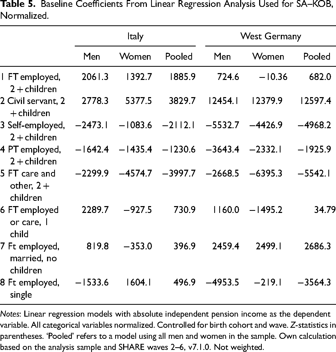
Notes: Linear regression models with absolute independent pension income as the dependent variable. All categorical variables normalized. Controlled for birth cohort and wave. Z-statistics in parentheses. ‘Pooled’ refers to a model using all men and women in the sample. Own calculation based on the analysis sample and SHARE waves 2–6, v7.1.0. Not weighted.

Interestingly, the male majority life courses which drive the GPG differ most between both countries. While the lack of women in the standard life course of men (cluster 1) is only significantly associated with a higher GPG in Italy (9.3%, €621 per year), a large share of the West German gap is due to gender differences in having a civil servant career (10.7%, €1,401). On one hand, this highlights the particularly beneficial pension rights for German civil servants. On the other hand, the contrasting results across countries for cluster 1 results from the return for men to this life course being much lower in West Germany compared to Italy (Table 5). This leads to a much lower explained share due to gender differences in cluster 1. Second, this life-course cluster contains a relatively high share of divorced men in Germany (Table A5.1 in the supplemental material), which likely decreases the average return to this life course for men due to the splitting of pension rights after divorce (Kreyenfeld et al. 2022).

GPGs are largely driven by the under- or overrepresentation of women in life-course clusters that include parenthood (clusters 1–5). In line with recent research on the US (Fasang and Aisenbrey 2022), this highlights the crucial role of the gendered interplay of work and family over the life course. Other scholars have highlighted the importance of parenthood for women's financial security in old age (e.g., Crespi et al. 2015). But the multichannel SA–KOB decomposition uniquely detects and quantifies the extent to which the interdependence of work and family life courses evident for women, but not for men, drives the GPGs in different welfare state contexts.

In sum, equalizing gendered work–family life courses, or the pension returns to the gender-specific life courses, would lead to an increase in pensions of €2,106 per year for women in Italy (175 euros per month) and of €3,476 per year (€289 per month) in West Germany. To put these numbers in perspective for the Italian case, one could consider, for example, that eliminating 30% of the GPG (keeping men's pensions constant) would lead to an increase in women's pension of an amount corresponding roughly to one third of the absolute poverty threshold (set at €700 per month for a single person aged 60–74, data from ISTAT 2021). This is substantively relevant from a social policy perspective, also given that women's old-age poverty risk exceeds men's by far in most European countries, including Germany and Italy (Haitz 2015).

Turning to the returns component of the unexplained shares of the SA–KOB decomposition, Figure 3 displays the shares arising from differences in pension income returns for membership of the same life-course cluster. GPGs are much less related to differences in returns to the same work–family life-course clusters than compositional differences of men and women experiencing different life-course clusters. ¹⁹ The sum of different rewards for the same life-course clusters only account for 5.8% of the GPG in Italy and 4.2% in West Germany. In both countries, the main driver is the life-course cluster characterized by having one child in marriage coupled with full-time employment in the private sector (Italy: 7.2%, €478; West Germany: 4%, €518). Alternatively, such differences in returns might be a result of gender-sensitive redistribution in the pension system favoring men, a high degree of gender-specific within-cluster heterogeneity (suggested by our sensitivity analysis), or gender-specific labor-market outcomes that affect pension income and are not controlled for (e.g., earnings, occupational segregation).

Figure 3.

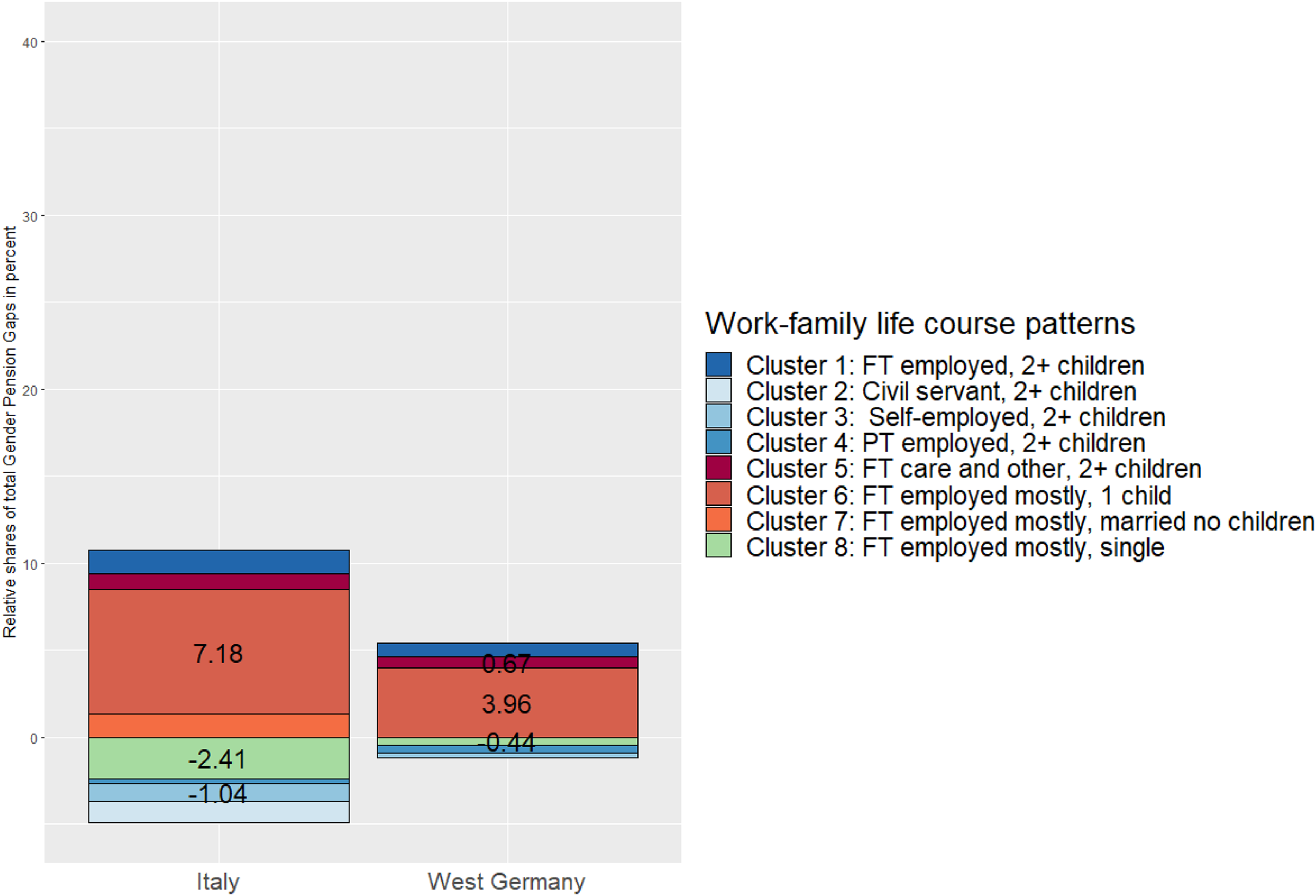
Decomposition results – shares from returns component of the unexplained part by work–family life courses and country. Notes: Percent of shares only displayed if minimum significance level of 10%. Results from KOB decompositions from Table 4. Based on normalized linear regression models with absolute independent pension income as dependent variable. Adjusted for birth cohort und wave. Confidence intervals depicted in Figures S5.1 and S5.2 in the Supplementary Materials. Own calculation based on the analysis sample and SHARE waves 2–6, v7.1.0. Not weighted.

Our findings thus suggest that modifying pension regulations—without fundamentally changing the entire pension system—is much less effective than comprehensive gender equality and work–family reconciliation policies.

Comparison of SA–KOB With Standard KOB Using Life Course Summary Measures

Empirically comparing the results of the SA–KOB with the standard decomposition approach using one-dimensional summary indicators as proxies for family and work life courses (the standard model) allows us to identify the benefits and limitations of both modeling approaches. We compare the results and discuss the benefits and limitations in detail in the Supplementary Materials E2 and Table A7 and summarize the main conclusions here.

Both modeling approaches have their strengths and weaknesses. The standard approach reveals the association of a limited number of specific and theoretically preselected life-course aspects with the GPG. The main limitation of SA–KOB is within-cluster heterogeneity, which might conceal the association with specific life-course aspects within the clusters. This might be the case for less prevalent life-course states that could either be concealed by more dominant life-course states within single clusters or could be distributed across different clusters (e.g., in our case, unemployment in cluster 4, duration of education in cluster 2, or duration of divorce in clusters 1, 2 and 6 in the SA–KOB).

However, the SA–KOB decomposition has important theoretical and empirical implications especially when the aim is to show how typical life-course patterns are rewarded (here: in pension systems) and consequently related to gaps in outcomes. First, SA–KOB allows us to include a multitude of different (categorical) life-course states and thus efficiently circumvents multicollinearity issues, whereas standard KOB is prone to multicollinearity and therefore has to use a limited number of life course covariates. In our case, for example, we had to exclude the duration in unpaid care work due to multicollinearity. As a consequence, the conclusion of the standard approach would be, in line with previous literature, that the highest shares of the GPG can be explained by the lack of women in employment. However, the SA–KOB decomposition points out that this is most likely rather driven by mothers with very few years in full-time employment before taking up unpaid care work for a long period, if not for the rest of their lives. SA–KOB more accurately highlights the dynamics behind women's fewer years in full-time employment. The continuous unpaid care-work provided by these mothers upon family formation prevents them from having as many years in full-time employment as fathers and means they do not have higher pensions in old age due to low returns to care-dominated life courses.

Second, if, in the standard model, one cannot include all life course summary measures due to multicollinearity, the selection of specific variables to be included in the model depends largely on the researcher's decision. This also poses the question of whether the life-course variables selected are indeed the most important predictors of the outcome of interest (here: mostly the duration in employment for the GPG, Table A1).

Third, summary measures are likely to conceal how different life-course clusters unfold their associations with inequalities through the order in which only certain life-course states appear along individual trajectories allocated to a given cluster. For example, only SA–KOB shows that part-time employment typically follows family-related employment interruptions as displayed by cluster 4. Therefore, SA–KOB demonstrates that, when considered in this combination with family-related employment interruptions, part-time employment is counterproductive for women's pension income whereas the standard approach suggests that more years in part-time employment benefit women's pension incomes.

Finally, the standard approach does not show the role of the relationship over time between different life-course domains. Only the SA–KOB decomposition (using MSA) reveals that the GPG is almost exclusively driven by the life courses of parents of at least two children as well as the importance of the intersections between work and family life courses that only occur for women.

We conclude that SA–KOB is particularly beneficial if researchers want to understand inequality-generating mechanisms in greater complexity than can be offered by simplified and unidimensional proxies for life courses due to SA–KOB's capacity to consider more life-course states simultaneously and capture (multidimensional) life-course complexities. This becomes more important the more complex and interdependent the life-course domains of interest are and the more this varies between the groups of interest (in our illustration women and men).

Discussion and Conclusions

In this study, we propose a novel combination of SA and KOB to offer a life-course sensitive analysis of group inequalities in outcomes that for the first time allows researchers to distinguish composition and return effects. To illustrate the potential of this approach and derive a set of practical guidelines, we have presented an illustrative application on work–family life courses to GPGs in Europe, a field that requires further social-policy research in view of population aging, changing family demographics and persistent gender inequalities in old age (Kuitto, Kuivalainen, and Möhring 2021).

Our contribution is twofold: methodological and substantive. The methodological contribution consists of the introduction of the stepwise SA–KOB decomposition. This is accompanied by detailed guidelines for making core decisions when applying the two analytical steps. These practical guidelines should facilitate applications of SA–KOB decomposition in other fields of research and inform some issues that apply to either method separately as well as to SA–KOB specifically. For example, we provide a systematic comparison of the most popular options for choosing the reference coefficients for KOB regarding the fit with SA–KOB and propose an option that is particularly well-suited to SA–KOB decomposition, that is, choosing the reference coefficients for clusters separately. We outline practical guidelines with regard to cluster-specific reference coefficients that are partly relevant for standard KOB applications as well. An additional benefit of SA–KOB decomposition is that researchers can use a set of established tools in SA for quantifying and visualizing within-cluster heterogeneity—an issue that applies to covariates in standard SA–KOB applications but has not received much attention so far. We suggest that these tools should guide the interpretation of the KOB estimates. For example, our application suggests that the explained shares tended to be underestimated, because the pension rewards of life-course clusters were obscured by life courses that were poorly assigned to specific clusters. Carefully considering within-cluster heterogeneity in SA applications is important more generally—poorly classified trajectories risk biasing the effect sizes of associations with sequence clusters, or, in severe cases, concealing associations entirely. Further, SA–KOB decomposition provides research on inequalities in life-course sensitive outcomes with a tool to bypass multicollinearity while still considering multiple life courses’ characteristics in decomposition analyses.

The explained part of the decomposition quantifies the role of the group-specific life courses for group inequalities in the outcome of interest. The returns component calls attention to group-specific inequalities in outcomes despite having the same trajectory pattern. We argue that SA–KOB decomposition adds to recent methodological advances in the field of sequence analysis that combine SA with other methods to improve the capacity of SA to address a wider range of research questions (see Liao et al. 2022 and Raab and Struffolino 2022 for a review).

Our second contribution is a substantive one, as we provide new insights on how gendered work–family life courses are associated with GPGs across welfare states. As we show by systematically comparing SA–KOB and the standard KOB approach (using life-course summary indicators), these substantive new insights emerge from the ability of SA–KOB to overcome the methodological flaws of previous studies that adopt the standard KOB approach. SA–KOB combines a multiverse of work and family life courses and at the same time bypasses the multicollinearity issue that arise when including several summary variables in the model to account for different life-course characteristics. By relying on such simplifying summary measures, the standard approach risks concealing some important inequality-generating dynamics that unfold across time.

SA–KOB enabled us to distinguish the part of the GPG that is due to gender differences in typical life-course clusters (the explained or compositional part) and the part that arises due to gender differences in pension returns for the same life-course clusters (the returns component of the unexplained part). Findings from the first step, the MSA, consistently show strongly gendered life-course clusters in line with the conservative welfare states of Germany and Italy. While fathers can reconcile parenthood with continuous employment, mothers either experience volatile employment life courses dominated by part-time jobs or fully dedicate their lives to lifelong unpaid care work in our study cohorts. Strong relationships between work life and parenthood only exist for life courses that are experienced mostly by women, and the gender differences in these life courses drive the GPG. The SA–KOB decomposition shows that GPGs in both countries are much more strongly associated with gender segregation in life-course clusters that are differently rewarded by the pension system (compositional component) than with different pension rewards between men and women for the same work–family life-course clusters (returns component). In both countries, the lack of full engagement in lifelong care work by fathers is the main driver of the gap. Thus, the high GPGs in Italy and West Germany are produced by the interrelation of different welfare policies that first shape the high level of gender differences in life courses and then reward these life courses unequally, to the detriment of women.

Thus, from a social policy perspective, SA–KOB decomposition informs intertemporal linkages between policy fields that first shape gendered life courses, and then decades later, pension rewards related to these life courses. The difference between compositional and returns effects cannot be interpreted in causal terms, but it can inform social policy, which generally has to rely on descriptive evidence concerning questions that do not lend themselves to experimental designs or methods for causal inference. One of these questions concerns how the timing, sequencing, and occurrence of events that unfold over several decades are associated with group inequalities in later life. The elements of the pension systems put in place to address gender inequalities (e.g., care benefits) are apparently too insignificant to lead to a reduction of the GPGs by offering better rewards for life courses characterized by care work periods (returns component). We follow previous findings in pointing out the insufficiency of care benefits in current pension systems (Abatemarco and Russolillo 2022; Frommert and Strauß 2013; Lis and Bonthuis 2019)—at least for the highly gendered contexts of Italy and West Germany for our study cohorts. Given that compositional life-course differences are the main driver of the GPG in Italy and Germany (explained part), policies that equalize access to different life-course types and reduce the strong interrelation between work and family lives for women are the most promising way to reduce the GPG. Such policies generally include defamilizing policies, such as public childcare, well-paid parental leave of about 1 year, and the abolition of joint couple's taxation (e.g., Adema, Clarke, and Thévenon 2020; Ferragina 2019; Ferragina and Seeleib-Kaiser 2015; Leitner 2001; Zagel and Lohmann 2020). Thus, policymakers in charge of retirement policies need to also consider policies affecting prime-age adults to ensure that women and men enjoy equal and fair financial security in old age.

Our illustrative application is subject to data constraints as, for example, it lacks annual information on other categories that are likely to be relevant for pension income, such as earnings, industries, and occupations. Some possible extensions of SA–KOB exist, especially with regard to exploring different decomposition techniques in combination with SA. First, our analysis focuses on group differences at the mean. However, mechanisms shaping inequalities are likely to differ along the distribution. This is also the case for GPGs (e.g., Hänisch and Klos 2014; Nolan et al. 2019). A combination of SA with decompositions along the distribution (for an overview: Fortin et al. 2011) was recently proposed by Gruijters, Van Winkle, and Fasang (2023). Second, applying Ñopo's decomposition to address the common support problem by using matching procedures might reveal further inequality dimensions like social closure for group differences (Ñopo 2008; Sprengholz and Hamjediers 2022). Finally, SA–KOB decomposition does not uncover causal effects as the KOB by design is not causal (Yu and Elwert 2023). However, recent methodological advances in both the decomposition (Jackson and VanderWeele 2018; Lundberg 2022; Yu and Elwert 2023) and the SA literature (Barban et al. 2020; Lee, Smith, and Galster 2017; for an overview: Raab and Struffolino 2022, chapter 7.4) have advanced both approaches in a causal manner. Future research should explore whether these approaches can be combined in a more causal SA decomposition. Given the caveats on causal interpretation, skepticism on whether any policy conclusion can be drawn based on standard KOB decompositions is merited (Yu and Elwert 2023). However, descriptive evidence on the complex mechanisms generating inequalities is key information that should not be discarded when designing policies, especially concerning research questions that are not amenable to research designs for causal inference from observational data for practical or ethical reasons. SA–KOB provides such policy-relevant findings by showing, for example, how much redistribution current pension regulations would have to undertake to compensate for pension inequalities resulting from prior gendered life courses.

To conclude, the proposed SA–KOB decomposition provides new insights into the extent of inequality in outcomes between groups associated with previous trajectories. As such, it holds potential for applications beyond later-life inequalities, for example, considering outcomes at early life stages and their association with prior educational trajectories or sequences of family situations in which children grow up. Decomposing the gender, race, or educational wage, wealth, or health gap based on previous (family, work, or health) trajectories are other natural applications.

Supplemental Material

sj-pdf-1-smr-10.1177_00491241231224226 - Supplemental material for Life-Course-Sensitive Analysis of Group Inequalities: Combining Sequence Analysis With the Kitagawa–Oaxaca–Blinder Decomposition

Supplemental material, sj-pdf-1-smr-10.1177_00491241231224226 for Life-Course-Sensitive Analysis of Group Inequalities: Combining Sequence Analysis With the Kitagawa–Oaxaca–Blinder Decomposition by Carla Rowold, Emanuela Struffolino and Anette Eva Fasang in Sociological Methods & Research

Supplemental Material

sj-pdf-2-smr-10.1177_00491241231224226 - Supplemental material for Life-Course-Sensitive Analysis of Group Inequalities: Combining Sequence Analysis With the Kitagawa–Oaxaca–Blinder Decomposition

Supplemental material, sj-pdf-2-smr-10.1177_00491241231224226 for Life-Course-Sensitive Analysis of Group Inequalities: Combining Sequence Analysis With the Kitagawa–Oaxaca–Blinder Decomposition by Carla Rowold, Emanuela Struffolino and Anette Eva Fasang in Sociological Methods & Research