Sage Journals: Discover world-class research

Abstract

The Kitagawa–Oaxaca–Blinder decomposition approach has been widely used to attribute group-level differences in an outcome to differences in endowment, coefficients, and their interactions. The method has been implemented for Stata in the popular oaxaca command for cross-sectional analyses. In recent decades, however, research questions have been more often focused on the decomposition of group-based differences in change over time, for example, diverging income trajectories, as well as decomposition of change in differences between groups, for example, change in the gender pay gap over time. We review five existing methods for the decomposition of changes in group means and contribute an extension that takes an interventionist perspective suitable for applications with a clear before–after comparison.

These decompositions of levels and changes over time can be implemented using the xtoaxaca command, which works as a postestimation command for different regression commands in Stata. It is built to maximize flexibility in modeling and implements all decomposition techniques presented in this article.

Keywords

st0640 xtoaxaca decomposition longitudinal data panel data Oaxaca Blinder Kitagawa

1 Introduction

The decomposition of group differences in means (Kitagawa 1955; Oaxaca 1973; Blinder 1973) is a popular tool when researchers seek to attribute such differences to differences in the groups’ characteristics and an unexplained part. As such, scholars have applied such decompositions to a variety of topics such as gender income inequality (Blau and Kahn 2017), happiness (Arrosa and Gandelman 2016), or obesity (Taber et al. 2016). This approach has also seen numerous extensions over the last decades to suit researchers’ needs, such as its application to distributional parameters other than the mean (Freeman 1980, 1984), to nonlinear models (Fairlie 2005; Bauer and Sinning 2008), to quantile regression (Machado and Mata 2005), to selection models (Neuman and Oaxaca 2003), and to other topics (for an overview, see Fortin, Lemieux, and Firpo [2011]). In large parts of the applied literature, these kinds of decompositions are known as Oaxaca–Blinder decompositions, after two of the three scholars who pioneered these approaches (Oaxaca 1973; Blinder 1973). We refer to this way of decomposing group mean differences as the Kitagawa–Oaxaca–Blinder (KOB) approach to reference the earliest and often overlooked contribution to this literature as well (Kitagawa 1955).

As researchers became increasingly interested in research questions involving developments over time, further extensions were developed to decompose the changes in mean group differences between two points in time (Smith and Welch 1989; Wellington 1993; Makepeace et al. 1999; DeLeire 2000; Kim 2010). These decomposition techniques are based on principles similar to those in the original KOB decomposition and have been primarily used in repeated cross-sectional studies on income gaps. None of those approaches mentioned above have been coherently implemented in Stata. We therefore propose the xtoaxaca command. It implements extensions of the original KOB decomposition that focus on the decomposition of changes between groups across time and makes decompositions available for pooled cross-section and panel data.

The command enables a user-friendly implementation of five existing decomposition methods for change (Smith and Welch 1989; Wellington 1993; Makepeace et al. 1999; DeLeire 2000; Kim 2010) and retains the possibility of applying it to panel data instead of only repeated cross-sectional regression models. It provides a generalization of the existing oaxaca command (Jann 2008) to longitudinal and panel data. It also includes a modified version of an existing decomposition approach (Wellington 1993), which is suitable for easy interpretation of the results under an interventionist perspective. This approach is aimed at before–after comparisons such as settings of interventions, policy changes, or (natural) experiments with a posttreatment follow-up. We believe that, in many instances, this perspective is applicable to numerous applied research settings in social sciences and has a more natural interpretation than the existing five decompositions of group differences in change over time.

The purpose of this article is to introduce both the xtoaxaca command for Stata and the new decomposition approach for change. In the next section, we introduce the concepts of longitudinal decompositions of levels and change of mean group differences over time. Both decompositions are implemented in the xtoaxaca command. We then elaborate on cross-sectional decomposition of levels—recapitulating the original KOB decomposition—and apply these principles to the decomposition of levels over time using longitudinal and panel data. The fourth section presents a discussion of different approaches to the decomposition of change. Thereafter, in the fifth section, we argue that an interventionist perspective on the decomposition of change has a crucial advantage in terms of interpretation for applied research. We then describe in the sixth section the syntax and options of the new xtoaxaca command. We present three empirical examples in the seventh section. The eighth section summarizes the main limitations of the xtoaxaca command. The last section concludes and provides an outlook for future research.

2 Decomposition of levels and change

Generally speaking, there are two ways in which we can use mean decomposition techniques with longitudinal data.

The first way of exploiting longitudinal data examines the contribution of past changes or events to levels of outcome differences between two groups A and B at a single time t_u . The second way is the decomposition of group differences in change in an outcome between two groups A and B between times s and t. We address both approaches in turn but highlight the importance of the latter.

Using longitudinal data to determine the contribution of past changes, we ask a typical research question:

1. How much of the difference in an outcome Y between groups A and B at time t is due to the differences in the incidence of a past event X, its different effects, or its different cumulative effects over the last n years?

This type of question utilizes longitudinal data by accounting for individuals’ past experiences. For instance, we may ask to what extent differences in past unemployment spells and their cumulative impact affect the gender wage gap at time t. In figure 1, this would translate into the decomposition of the outcome difference at t_u , ΔY_t . It would account for the different incidences and effects of events at r and u to explain the level difference ΔY_t . Analytically, this type of question is still cross-sectional in nature, and we can examine it using the traditional KOB decomposition.¹

In the following, we denote the repeated decomposition of group differences over time as the longitudinal decomposition of levels over time. Decomposing levels is a distinct approach from the second way of using longitudinal data for decomposition, the decomposition of change.

Figure 1.

Decomposition of changes over time

If we seek to decompose the change in mean group differences over time, we compare the mean group differences between groups A and B between two points in time, s and t, and ask what factors narrowed or widened the outcome difference over time. For example, the wage gap between men and women may have decreased over the last 10 years. A researcher might ask whether this occurred because of compositional changes (differential changes in endowments of the groups) or changes in the contribution of coefficients of the two groups. Thus, the second kind of longitudinal question can be expressed as follows:

2. How much of the change in differences in an outcome Y between groups A and B and between times t and s is due to changes in the groups’ composition or the effects of the explanatory variables?

In figure 1, this amounts to decomposing the change in group differences between time s and t, ΔY ^B − ΔY ^A .

As has been shown (Smith and Welch 1989; Wellington 1993; Makepeace et al. 1999; DeLeire 2000; Kim 2010), this type of question can be answered with repeated cross-sectional data. In this article, we demonstrate that these existing approaches to the decomposition of change can be easily generalized to the use of panel regression models as well. We argue, however, that the existing approaches are not always easy to interpret when asking a set of research questions that falls under what we call the interventionist perspective. Therefore, we argue that they can be usefully complemented by a new approach to the decomposition of change, which we lay out in detail in section 5.

3 Decomposition of levels

3.1 The KOB decomposition for cross-sectional data

Before we review the existing approaches to the decomposition of change, it is useful to recapitulate what the original KOB decomposition does using cross-sectional data (Kitagawa 1955; Oaxaca 1973; Blinder 1973). We will also introduce the notation we will use throughout the article. We start with a basic linear regression model for an outcome Y and two groups A and B:

Y_{t}^{l} = X_{t}^{l} β_{t}^{l} + ϵ_{t}^{l}, E (ϵ^{l}) = 0, cov (X, ϵ) = 0 l \in [A, B]

X represents the matrix of covariates, including the unity vector, while β contains the k − 1 coefficients and the constant, t denotes the time, and ǫ is the error term. The basic KOB decomposition applies to data with one time point and divides the mean outcome difference between the two groups into a part that is explained by differences in the groups’ characteristics and an unexplained part (twofold approach). Given that the decompositions of change we introduce in section 4 are often based on the assumption that there are group differences in the coefficients (threefold decomposition), we illustrate our notation on this approach. Given the outcome difference

\begin{matrix} Δ Y_{t} = E (Y_{t}^{A}) - E (Y_{t}^{B}) \\ = E (X_{t}^{A}) β_{t}^{A} - E (X_{t}^{B}) β_{t}^{B} \end{matrix}

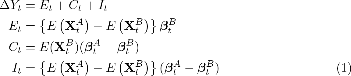
and given that $E (X_{t}^{l} β_{t}^{l} + ϵ_{t}^{l}) = E (X_{t}^{l} β_{t}^{l})$ , the outcome difference can be decomposed into

\begin{matrix} Δ Y_{t} = E_{t} + C_{t} + I_{t} \\ E_{t} = {E (X_{t}^{A}) - E (X_{t}^{B})} β_{t}^{B} \\ C_{t} = E (X_{t}^{B}) (β_{t}^{A} - β_{t}^{B}) \\ I_{t} = {E (X_{t}^{A}) - E (X_{t}^{B})} (β_{t}^{A} - β_{t}^{B}) \end{matrix}

E_t is defined as the part of the difference that is due to differences in the groups’ characteristics at time t (endowments effect). C_t is the part of the difference that is due to differences in the coefficients at time t. I_t , finally, is the part of the difference at time t that is due to the interaction of the groups’ different characteristics and coefficients.

The presented decomposition in (1) is a threefold decomposition from the viewpoint of group B, meaning that E_t is weighted by B’s coefficients and that C_t is weighted by B’s characteristics. While this suffices to represent the basic principle of the KOB decomposition, other decompositions such as a twofold decomposition or a decomposition from the viewpoint of group A are possible (compare with Jann [2008] and Fortin, Lemieux, and Firpo [2011]).

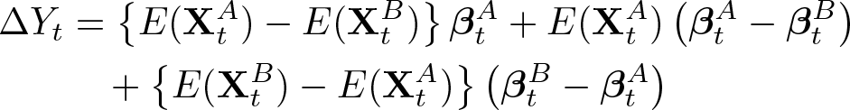
From the viewpoint of group A, we would weight the differences in characteristics and coefficients with the characteristics and coefficients of group A instead of group B:

\begin{matrix} Δ Y_{t} = {E (X_{t}^{A}) - E (X_{t}^{B})} β_{t}^{A} + E (X_{t}^{A}) (β_{t}^{A} - β_{t}^{B}) \\ + {E (X_{t}^{B}) - E (X_{t}^{A})} (β_{t}^{B} - β_{t}^{A}) \end{matrix}

For the twofold decomposition, which is the one originally devised by Oaxaca and Blinder, the outcome difference (with group A as the reference) is decomposed by

Δ Y_{t} = {E (X_{t}^{B}) - E (X_{t}^{A})} β_{t}^{A} + E (X_{t}^{B}) (β_{t}^{B} - β_{t}^{A})

This is also implemented in xtoaxaca but not discussed in detail in this article. Normalization of explanatory variables (Yun 2005) has also been implemented as explained in the next section, 3.2.

3.2 Normalization of categorical variables

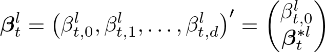
As has been noted in the literature (Jann 2008; Kim 2010; Yun 2005), there is an identification problem when categorical variables are used for decomposition. A widely used solution is to normalize the coefficients of categorical variables by subtracting the variable-specific mean of the coefficient from each category of the variable-specific coefficients and adding all subtracted means to the intercept for decomposition purposes. This yields a new set of coefficients for the decomposition defined as

{\tilde{β}}_{t, j}^{l} = β_{t, j}^{l} - \frac{\sum_{i}^{c} β_{t, j, i}^{l}}{c}

In this notation, j indicates the jth categorical variable and c the cth category within the jth categorical variable, with β_t,j, ₁ constrained to zero for identification in the original model. The time-specific intercept is then defined as

{\tilde{β}}_{t, 0}^{l} = β_{t, 0}^{l} + \sum_{i = 1}^{j} \frac{\sum_{h = 1}^{c} β_{t, i, h}^{l}}{c} = β_{t, 0}^{l} + {\bar{β}}_{t}^{l}

As can be seen, the basic principle of the original KOB decomposition is to get counterfactual estimates for the outcome, for example, group B, assuming it had the same endowments or coefficients as group A. This reasoning is retained in the decomposition of levels and change over time as well.

3.3 Longitudinal data using nonpanel regression models

The use of the KOB decomposition with nonpanel regression models is unproblematic with longitudinal data as long as time is measured discretely. Discretely in this context means that observations are categorized together to have been observed at the same undifferentiated time point, for example, in waves of a cohort of panel study. In this case, the analysis is identical to a repeated cross-sectional approach. However, the assumption can also be that the time variable is (quasi)continuous. In this case, we have to define a bandwidth (b) around the time points to allow for an estimation of the endowments part. The wider the bandwidth is, the more reliable the estimate is because more data points fall into the bandwidth around the time point (and the smaller the standard errors become). Broadening the bandwidth comes at the price of losing sensitivity to time-dependent changes in the endowment. For nonparametric modeling, this is similar to the tradeoff that has to be made between bias and variance (Härdle et al. 2004, 28). We estimate

E (X_{t - b; t + b}^{l})

The subscript t − b refers to the lower bound and t + b refers to the upper bound of the interval on the time variable that is used to estimate the mean of the variables. In the case of the continuous-time variable, the decomposition components become a function of the chosen bandwidth b.

This raises the question of whether the coefficients, like the endowment, can also become dependent on the chosen bandwidth. This has to be decided in line with the choice of the functional form of the time variable in the regression models used for the decomposition. Even when a bandwidth of some kind is used for the endowments, a parametric form can be chosen for the coefficients over time. However, the time variable can be constructed to reflect the bandwidth around prespecified points in time. In such a case, the coefficients can be estimated nonparametrically for each of these time intervals separately, and the decomposition can be done for each of these time intervals. Under these circumstances, coefficients and endowments would be treated analogously.

For simplicity’s sake, we leave out the bandwidth in the index for the remainder of the article, but note that it is theoretically necessary and practically possible to set the bandwidth in cases in which time is assumed to be continuous.

3.4 Longitudinal data using panel regression models

Using panel data, we can also estimate β from a panel regression model. Because panel regressions model time-constant individual error terms, a decomposition using panel regression models must account for empirical group differences in these time-constant, unobserved variables. Thereby, the time-constant individual error terms u ^l become part of the decomposition of group-level differences.

Y_{t}^{l} = X_{t}^{l} β_{t}^{l} + u^{l} + ϵ_{t}^{l}, E (ϵ_{t}^{l}) = 0, cov (X_{t}, ϵ_{t}) = 0 l \in [A, B]

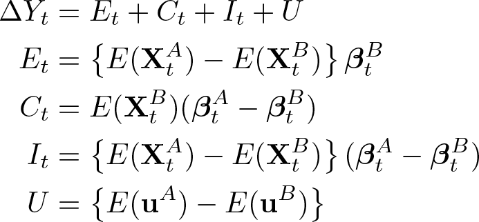
Accounting for the time-constant error terms adds the differences in the expectation of u ^l as a fourth component U to the decomposition. This component is not time dependent. It only comprises differences between groups in the time-constant error terms.²

\begin{matrix} Δ Y_{t} = E_{t} + C_{t} + I_{t} + U \\ E_{t} = {E (X_{t}^{A}) - E (X_{t}^{B})} β_{t}^{B} \\ C_{t} = E (X_{t}^{B}) (β_{t}^{A} - β_{t}^{B}) \\ I_{t} = {E (X_{t}^{A}) - E (X_{t}^{B})} (β_{t}^{A} - β_{t}^{B}) \\ U = {E (u^{A}) - E (u^{B})} \end{matrix}

Accordingly, a decomposition using panel regression models attributes parts of the differences between groups to unobserved factors that do not change within the period of observation.

3.5 Model assumptions

Selection and causal identification

Note that any results produced by decompositions of levels or change rely on the assumptions made in the original regression models. This pertains especially to the causal interpretation of the results. Following a counterfactual interpretation of causality in the social sciences (Morgan and Winship 2015), the estimators for the explanatory variables would need to be unbiased. Only then could the results of any of the decomposition approaches presented here (including the original KOB decomposition) be given interpretations like “how much would the gap between group A and group B be reduced if group A had the same endowments as group B?” Panel regression models offer some advantages when it comes to arguing that the assumptions for causal interpretation are fulfilled but still rest on certain assumptions that are often not realistic in applied research (Firebaugh, Warner, and Massoglia 2013).

For example, from a more technical perspective, note that in a standard randomeffects model (which includes the grouping variable l as a covariate), the assumption is that cov(l, u) = 0. This implies that E{E(u ^A ) − E(u ^B )} = 0. If our model conforms to this assumption, we should therefore expect that the time-constant error terms cannot contribute to the explanation of differences in group levels of the outcome. If we see strong deviations in an empirical estimation of E{E(u ^A ) − E(u ^B )} = 0, this might indicate a misspecified model leading to biased coefficient estimates, which in turn could lead to a biased decomposition.

Panel dropout

With longitudinal data, panel dropout is a serious issue that may affect the estimation of coefficients (Oaxaca and Choe 2016) as well as the estimation of the time-specific endowment component. If the results are to be interpreted causally, endogeneity problems resulting from panel dropout have to be solved when designing the panel regression models before the decomposition is applied.

It is possible for dropout rates to differ between the groups under study. This can also affect the estimation of the endowments in (3). To avoid biased endowment estimators, one must construct weights that account for the effects of differential panel dropout and applied them in the estimation of the endowments. How these are constructed is beyond the scope of this article; however, we recommend standard procedures from the literature on survey research (Kalton and Flores-Cervantes 2003; Deming and Stephan 1940; Kim and Kim 2007), which can be implemented in Stata using survwgt (Winter 2002).

Functional form of the time variable

In the modeling process, one can either specify time nonparametrically, estimating an interaction of each time point with the group variable and each decomposition variable, or assume a certain functional form like linear growth. The decomposition will rely on these assumptions made in the modeling process. If the functional form is chosen incorrectly, this will also affect the decomposition, and the results will consequently be biased. This is important not only for the overall growth of the dependent variable but also for the change in the effect of the decomposition variables over time. A nonparametric approach is less statistically efficient but has much weaker assumptions than any parametric function and might therefore be preferred if researchers are uncertain in this regard.

3.6 Decomposition in a multilevel framework

Because all panel models can be understood as a special case of multilevel models (with time points nested within units), we believe that xtoaxaca can also be used to decompose levels and differences³ between clusters or higher-level units. Thus, the time variable needs to reflect the cluster variable (for example, countries) and should be used in categorical interaction with the desired variables in the model. Differences between units in a multilevel framework and differences between time points can both be seen as a form of difference-in-differences decomposition.

The interpretation of the decomposition of levels over different clusters does not deviate from repeated cross-sectional KOB decompositions, and so using xtoaxaca would not contribute much extra benefit over using oaxaca. However, decomposition of difference in differences between groups over clusters or higher-level units might be of interest (Blau and Kahn 1992). The interpretation then refers to whether differences between clusters or higher-level units in the group differences in the outcome can be attributed to cluster differences in the group differences in endowments, coefficients, or their interactions.

4 Decomposition of change

Regardless of whether we have repeated cross-sectional or panel data, given two groups A and B for which we have data for at least two points in time, t and s with t > s, the change in the outcome difference between the two groups and between the two points in time is given by

Δ Y = Δ Y_{t} - Δ Y_{s}

Alternatively, changes in outcome differences between two groups and two points in time can be expressed as the difference of group differences over time:

\begin{matrix} Δ Y = Δ Y_{t} - Δ Y_{s} \\ = (E (Y_{t}^{A}) - E (Y_{t}^{B})) - (E (Y_{s}^{A}) - E (Y_{s}^{B})) \\ = E (Y_{t}^{A}) - E (Y_{t}^{B}) - E (Y_{s}^{A}) + E (Y_{s}^{B}) \\ = E (Y_{t}^{A}) - E (Y_{s}^{A}) - E (Y_{t}^{B}) + E (Y_{s}^{B}) \\ = E (Y_{t}^{A}) - E (Y_{s}^{A}) - (E (Y_{t}^{B}) - E (Y_{s}^{B})) \\ = Δ Y^{A} - Δ Y^{B} \end{matrix}

Essentially, changes over time can therefore be expressed as the difference between two KOB decompositions at different time points.

Several approaches for the decomposition of change in group differences over time exist. We cover the five most prominent examples.⁴ These decompositions of change have been applied to both points using repeated cross-sectional data. The generalization of the decomposition of levels to continuous time and panel data introduced in the previous section applies in the same way to the decomposition of change as it does to the decomposition of levels.

4.1 Simple subtraction method (SSM)

The simplest decomposition of change is a simple subtraction of the decomposition components of the original KOB decomposition at time s from the components at time t and is defined in our notation as SSM:

\begin{matrix} Δ Y = Δ Y_{t} - Δ Y_{s} \\ = E_{t} + C_{t} + I_{t} - (E_{s} + C_{s} + I_{s}) = \\ (E_{t} - E_{s}) + (C_{t} - C_{s}) + (I_{t} - I_{s}) \\ = \underset{E_{t}}{\underset{︸}{{E (X_{t}^{A}) - E (X_{t}^{B})} β_{t}^{B}}} - \underset{E_{s}}{\underset{︸}{{E (X_{s}^{A}) - E (X_{s}^{B})} β_{s}^{B}}} \\ + \underset{C_{t}}{\underset{︸}{E (X_{t}^{B}) (β_{t}^{A} - β_{t}^{B})}} - \underset{C_{s}}{\underset{︸}{E (X_{s}^{B}) (β_{s}^{A} - β_{s}^{B})}} \\ + \underset{I_{t}}{\underset{︸}{{E (X_{t}^{A}) - E (X_{t}^{B})} (β_{t}^{A} - β_{t}^{B})}} - \underset{I_{s}}{\underset{︸}{{E (X_{s}^{A}) - E (X_{s}^{B})} (β_{s}^{A} - β_{s}^{B})}} \end{matrix}

This method is straightforward to calculate, applied for example in DeLeire (2000). The endowment part can be interpreted as the part in the change in the gap that is due to changes in the endowments given changes in the evaluation (coefficient) in the reference group over time. The coefficient part is the part in the change in the gap that is due to changes in the coefficients given changes in the evaluation (endowment) in the reference group over time. The interaction part is the difference in the interactions of group differences in coefficients and endowments. Similarly to the original KOB, this component is difficult to interpret and might often be treated as the substantively unexplained part.

The approach has also attracted criticism because it does not estimate the unique contribution of coefficient changes and changes in the variable distributions over time (Kim 2010). As Kim (2010) shows, the coefficient differences at each time point are weighted by the mean distribution of the endowments at their respective time and, because the endowments likely change over time, the coefficient effect captures these changes. Similarly, the endowment effect contains interactions between the coefficient and endowment changes. This kind of criticism applies differently for all the decompositions presented here, except for the one by Kim (2010).

4.2 Smith and Welch (1989)

Smith and Welch (1989) propose a fourfold decomposition of change that is defined in our notation as SW (Smith and Welch 1989, 529):

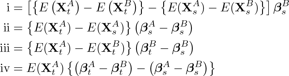
\begin{matrix} i = [{E (X_{t}^{A}) - E (X_{t}^{B})} - {E (X_{s}^{A}) - E (X_{s}^{B})}] β_{s}^{B} \\ ii = {E (X_{t}^{A}) - E (X_{s}^{A})} (β_{s}^{A} - β_{s}^{B}) \\ iii = {E (X_{t}^{A}) - E (X_{t}^{B})} (β_{t}^{B} - β_{s}^{B}) \\ iv = E (X_{t}^{A}) {(β_{t}^{A} - β_{t}^{B}) - (β_{s}^{A} - β_{s}^{B})} \end{matrix}

The components can be given the following interpretation:⁵

i. Main effect: The component estimates the predicted change in the outcome between the two groups that can be attributed to the two groups are changing in the endowments (valued at base time s) between time t and s.

ii. Group interaction: The second component describes the part of change in the endowment of the group that is valued differently at time s. Therefore, a secular rise in endowments gives a higher benefit to the group with the higher return to this endowment at time s.

iii. Time interaction: This component takes the endowment differences at the second time point and attributes change to the change in the coefficient of group B. This would mean that higher returns to an endowment benefit the group with higher endowments at time point t.

iv. Group-time interaction: The last component attributes change to a change in the differences in the coefficients (returns to endowments) given the initial level of group A. If group A were the disadvantaged group, reduction in the differences to the return to their endowments would close the overall gap between the groups.

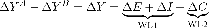
4.3 Wellington (1993)

Wellington (1993) proposes a simple twofold decomposition of change in differences in labor market returns. Her decomposition is defined in our notation as WL (Wellington 1993, 393):

\begin{array}{l} WL 1 = {E (X_{t}^{A}) - E (X_{s}^{A})} β_{t}^{A} - {E (X_{t}^{B}) - E (X_{s}^{B})} β_{t}^{B} \\ WL 2 = E (X_{s}^{A}) (β_{t}^{A} - β_{s}^{A}) - E (X_{s}^{B}) (β_{t}^{B} - β_{s}^{B}) \end{array}

Wellington (1993, 393–394) gives the following description of the two components:

WL1. The portion of the change in the gap that can be accounted for by changes in the means if the returns to the independent variables were constant at t (not at baseline s).

WL2. The portion of the change in the gap that can be explained by changes in the coefficients (including the constant term) over the period, evaluated at the groups’ baseline (s) means.

This approach is the one that is closest to our own addition (see next subsection) to the set of possible decomposition approaches, but there is a slight but significant difference, as we discuss in section 5.

4.4 A threefold extension of WL (interventionist)

There is another useful way in which the change in gaps can be decomposed. This is an extension of the WL decomposition, which takes the form of a threefold decomposition.

Δ Y^{A} - Δ Y^{B} = Δ Y = \underset{WL1}{\underset{︸}{Δ E + Δ I}} + \underset{WL2}{\underset{︸}{Δ C}}

The three components are named analogously to the original KOB decomposition. To obtain the endowments effect, we allow only the groups’ composition to vary over time and hold the coefficients constant at their initial group-specific levels at time s.

\begin{matrix} Δ E = E (X_{t}^{A}) β_{s}^{A} - E (X_{s}^{A}) β_{s}^{A} - E (X_{t}^{B}) β_{s}^{B} + E (X_{s}^{B}) β_{s}^{B} \\ = {E (X_{t}^{A}) - E (X_{s}^{A})} β_{s}^{A} - {E (X_{t}^{B}) - E (X_{s}^{B})} β_{s}^{B} \end{matrix}

As can be seen in (5), we obtain the endowments component by subtracting the groups’ compositional changes over time weighted by their initial coefficients. The endowments component then answers the following question: Given the initial differences in coefficients, how much does the gap between groups change because of the changes in the endowments between both points (if the coefficients do not change)?

Similar to the endowments effect, the component attributable to a change in coefficients is obtained by fixing the groups’ endowments so that $E (X_{t}^{l}) = E (X_{s}^{l})$ ,

\begin{matrix} Δ C = E (X_{s}^{A}) β_{t}^{A} - E (X_{s}^{A}) β_{s}^{A} - E (X_{s}^{B}) β_{t}^{B} + E (X_{s}^{B}) β_{s}^{B} \\ = E (X_{s}^{A}) (β_{t}^{A} - β_{s}^{A}) - E (X_{s}^{B}) (β_{t}^{B} - β_{s}^{B}) \end{matrix}

which denotes the change of the difference due to a change in coefficients (including the constant) over time between the groups given the groups’ initial differences in endowments at s. The coefficient component answers this question: Given the initial differences in endowments, how much does the gap between groups change because of changes in the coefficients (if the endowments do not change)?

The interaction between the change in endowments and coefficients is the last component of the decomposition:

Δ I = {E (X_{t}^{A}) - E (X_{s}^{A})} (β_{t}^{A} - β_{s}^{A}) - {E (X_{t}^{B}) - E (X_{s}^{B})} (β_{t}^{B} - β_{s}^{B})

As with the original KOB decomposition, it is difficult to give this component a straightforward interpretation on its own. Additionally, note that the subcomponent of ΔC that is attributable to a change in the intercept is usually also a kind of residual, unexplained by the (change in) X variables in the model.

We can show that our suggested approach is a direct extension of Wellington (1993). First, our ΔC component is exactly the same as WL2 of the Wellington decomposition.

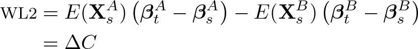
\begin{matrix} WL 2 = E (X_{s}^{A}) (β_{t}^{A} - β_{s}^{A}) - E (X_{s}^{B}) (β_{t}^{B} - β_{s}^{B}) \\ = Δ C \end{matrix}

In addition, if we add up the endowment and interaction term of the interventionist decomposition, we get the first part of the Wellington decomposition.

\begin{matrix} Δ E + Δ I = {E (X_{t}^{A}) - E (X_{s}^{A})} β_{s}^{A} - {E (X_{t}^{B}) - E (X_{s}^{B})} β_{s}^{B} + \\ {E (X_{t}^{A}) - E (X_{s}^{A})} (β_{t}^{A} - β_{s}^{A}) - {E (X_{t}^{B}) - E (X_{s}^{B})} (β_{t}^{B} - β_{s}^{B}) \\ = {E (X_{t}^{A}) - E (X_{s}^{A})} β_{t}^{A} - {E (X_{t}^{B}) - E (X_{s}^{B})} β_{t}^{B} \\ = WL 1 \end{matrix}

4.5 Makepeace et al. (1999)

Another well-known approach aims at partially mirroring the twofold cross-sectional KOB decomposition into explained and unexplained in the decomposition of change. The authors further divide the explained and unexplained components into a component related to change in endowments (pure) and one aspect related to change in coefficients (price) (Makepeace et al. 1999, 539). Their decomposition is defined in our notation as MPJD:

\begin{matrix} Δ E_{pure} = [{E (X_{t}^{A}) - E (X_{s}^{A})} - {E (X_{t}^{B}) - E (X_{s}^{B})}] β_{t}^{A} \\ Δ E_{price} = {E (X_{s}^{A}) - E (X_{s}^{B})} (β_{t}^{A} - β_{s}^{A}) \\ Δ U_{pure} = E (X_{t}^{B}) {(β_{t}^{A} - β_{s}^{A}) - (β_{t}^{B} - β_{s}^{B})} \\ Δ U_{price} = {E (X_{t}^{B}) - E (X_{s}^{B})} (β_{s}^{A} - β_{s}^{B}) \end{matrix}

4.6 Kim (2010)

While many decomposition approaches were developed with particular research questions in mind, Kim (2010) develops the most analytical approach. It yields five components, of which two can be attributed purely to the change in endowments and coefficients. He argues that all methods discussed so far in this article confuse or at least conflate the pure change in endowment and the pure change in the coefficients with interactions of such changes with initial (or current) level differences in coefficients and endowments. We agree with the analysis but argue in section 5 that for the sake of interpretability, this might be a desirable property of a decomposition.

To better understand how the KIM decomposition (Kim 2010, 629) decomposes group differences over time, we need to take the intercepts apart from the rest of the coefficients in this subsection. So far, decompositions have used the standard matrix notation of multiple regression. This means that the time-specific intercepts $β_{t, 0}^{l}$ are part of the coefficient vectors,

β_{t}^{l} = {(β_{t, 0}^{l}, β_{t, 1}^{l}, \dots, β_{t, d}^{l})}^{'} = (\begin{array}{l} β_{t, 0}^{l} \\ β_{t}^{* l} \end{array})

with d being the number of decomposition variables used in the model. Accordingly, the means matrices so far have contained a unity vector that is multiplied with the intercepts:

E (X_{t}^{l}) = {1, E (X_{t, 1}^{l}), \dots, E (X_{t, d}^{l})} = {1, E (X_{t}^{* l})}

Kim (2010) uses a different approach by explicitly distinguishing between intercepts and covariates. Therefore, the notation for the coefficients uses ${\tilde{β}}_{t}^{* l}$ to represent the coefficient vector without the intercept and $E (X_{t}^{* l})$ as the means vector without the 1. Additionally, the decomposition uses the normalization of categorical variables proposed by Yun (2005) (see section 3.2). After normalization, the vector of coefficients may contain normalized categorical and nonnormalized continuous variables. We distinguish categorical variables by counting them first in the set of coefficients until the total number of categorical variables j is reached. Continuous variables start with an index of j + 1 until they reach d, which is the total number of decomposition variables. Such an explicit distinction between continuous and categorical variables is not necessary for other sections of the article. The normalized (demeaned) vector of coefficients thus contains

{\tilde{β}}_{t}^{l} = {({\tilde{β}}_{t, 0}^{l}, {\tilde{β}}_{t, 1, c}^{l}, \dots, {\tilde{β}}_{t, j, c}^{l}, β_{t, j + 1}^{l}, \dots, β_{t, d}^{l})}^{'}

with j being the number of categorical variables, c indexing the categories of each categorical variable, ${\tilde{β}}_{t, 0}^{l}$ being the intercept for the demeaned coefficients [see (2)], ${\tilde{β}}_{t, 1, c}^{l}, \dots, {\tilde{β}}_{t, j, c}^{l}$ being the demeaned coefficients of the categorical variables, and ${\tilde{β}}_{t, j + 1}^{l}, \dots, {\tilde{β}}_{t, j, c}^{l}$ being the regular coefficients of the continuous variables. If we now take the normalized vector of coefficients and leave out the intercept ${\tilde{β}}_{t, 0}^{l}$ , we get ${\tilde{β}}_{t}^{* l}$ .

With the definition of normalization in section 3.2 and ${\tilde{β}}_{t}^{* l}$ being the normalized coefficient vector without the intercept, it follows that

\begin{matrix} E (X_{t}^{* l}) {\tilde{β}}_{t}^{* l} + β_{t, 0}^{l} + {\bar{β}}_{t}^{l} = {1, E (X_{t}^{* l})} (β_{t, 0}^{l}, {\tilde{β}}_{t}^{* l} + {\bar{β}}_{t}^{l}) \\ = E (X_{t}^{l}) β_{t}^{l} \end{matrix}

Taking these definitions into account, we define the five-part KIM decomposition in our notation as follows:

\begin{array}{l} D 1 = {(β_{t, 0}^{A} - β_{s, 0}^{A}) - (β_{t, 0}^{B} - β_{s, 0}^{B})} + {({\bar{β}}_{t}^{A} - {\bar{β}}_{s}^{A}) - ({\bar{β}}_{t}^{B} - {\bar{β}}_{s}^{B})} \\ D 2 = (\frac{E (X_{t}^{* A}) + E (X_{s}^{* A}) + E (X_{t}^{* B}) + E (X_{s}^{* B})}{4}) {({\tilde{β}}_{t}^{* A} - {\tilde{β}}_{s}^{* A}) - ({\tilde{β}}_{t}^{* B} - {\tilde{β}}_{s}^{* B})} \\ D 3 = (\frac{{E (X_{t}^{* A}) - E (X_{s}^{* A})} + {E (X_{t}^{* B}) - E (X_{s}^{* B})}}{2}) \\ (\frac{({\tilde{β}}_{t}^{* A} + {\tilde{β}}_{s}^{* A})}{2} - \frac{({\tilde{β}}_{t}^{* B} + {\tilde{β}}_{s}^{* B})}{2}) \\ D 4 = [{E (X_{t}^{* A}) - E (X_{s}^{* A})} - {E (X_{t}^{* B}) - E (X_{s}^{* B})}] (\frac{{\tilde{β}}_{t}^{* A} + {\tilde{β}}_{s}^{* A} + {\tilde{β}}_{t}^{* B} + {\tilde{β}}_{s}^{* B}}{4}) \\ D 5 = (\frac{{E (X_{t}^{* A}) + E (X_{s}^{* A})}}{2} - \frac{{E (X_{t}^{* B}) + E (X_{s}^{* B})}}{2}) \\ (\frac{({\tilde{β}}_{t}^{* A} - {\tilde{β}}_{s}^{* A}) + ({\tilde{β}}_{t}^{* B} - {\tilde{β}}_{s}^{* B})}{2}) \end{array}

Following Kim (2010), we can give the following descriptions of the five components:

D1 Intercept effect: This is purely the difference in differences between group and overall intercepts.

D2 Pure coefficient effect: This component measures how much the gap between groups changes because of changes in the coefficients if there were no differences in the endowments at all, neither between groups nor over time.

D3 Coefficient interaction effect: This component measures how much the gap between groups changes because of the average change in endowment combined with the difference in the averaged coefficient. It is supposed to capture the aspect of initial level differences in coefficients, which affect the change in the gap in interaction with changes in endowments.

D4 Pure endowment effect: This component is the analog to D2 for endowments. It measures how much the gap between groups changes because of changes in the endowments if there were no differences in the coefficients at all, neither between groups nor over time.

D5 Endowment interaction effect: This component is the analog to D3 but reverses the role of endowment and coefficients. It measures how much the gap between groups changes because of the average change in coefficients combined with the difference in the averaged endowments. It is supposed to capture the aspect of initial level differences in endowments, which affect the gap in interaction with changes in coefficients.

4.7 Panel models and time-constant error terms

As mentioned in section 3.4, decompositions can also attribute parts of group differences in levels of the outcome to factors that are time constant within the period of observation. The same can be done for change over time (ΔU). However, this makes sense only if we have an unbalanced panel. If the panel is balanced, the expectations of the time-constant error terms cannot change over time and cannot contribute anything to the decomposition of change between groups.

If we see substantial contributions of the time-constant error terms, the data suffer from group-specific panel attrition, which contributes to a change in the group differences in the outcome. In this case, we can add a component ΔU to all the previous five decompositions as well as to the interventionist decomposition method introduced in the next section.

Δ U = {E (u_{t}^{A}) - E (u_{s}^{A})} - {E (u_{t}^{B}) - E (u_{s}^{B})}

4.8 The relationship between the different types of decompositions

Because all decomposition approaches decompose the same differences in change over time, each decomposition can be expanded and transformed into any other of the existing decompositions. Nevertheless, there are some direct relationships that are worth mentioning and that are also depicted in figure 2.⁶

Figure 2.

Relationship among decomposition approaches. note: SSM = simple subtraction method (section 4.1), WL = Wellington (1993) (section 4.3), MPJD = Makepeace et al. (1999) (section 4.5), SW = Smith and Welch (1989) (section 4.2), KIM = Kim (2010) (section 4.6)

The six decomposition methods can be divided into a heuristic based on a combination of two characteristics. The first one is simply the number of components used. Here we see between two and five components. The second characteristic divides the methods into those that conduct decompositions groupwise across time and those that conduct decompositions timewise across groups. Timewise across groups means that the differences between groups at one time point are subtracted from the differences between groups from another time point. In contrast, groupwise across time means that the differences between time points within one group are subtracted from the differences between time points within the other group.

WL, KIM, and the interventionist approach fall clearly into the groupwise-across-time category, while SSM is a timewise-across-group approach. For MPJD and SW, not all components of their decomposition follow this logic. For MPJD, the pure components are groupwise across time, and for SW the components i and iv are timewise across group.

In section 4.4, we have already shown that WL can be further divided to yield a threefold decomposition that we label interventionist and that we argue has a certain desirable property in contrast with all other approaches, which we elaborate on in section 5.

The simple subtraction method does timewise subtractions across groups of the components of endowments, coefficients, and interactions. If we were to exchange time points with groups, we would end up with a groupwise subtraction across time. This is exactly what is done in the interventionist perspective. So if we were to substitute t = A and s = A, the equations would be

\begin{matrix} Δ E = E_{A} - E_{B} = {E (X_{A}^{t}) - E (X_{A}^{s})} β_{A}^{s} - {E (X_{B}^{t}) - E (X_{B}^{s})} β_{A}^{s} \\ Δ C = C_{A} - C_{B} = E (X_{A}^{s}) (β_{A}^{t} - β_{A}^{s}) - E (X_{B}^{s}) (β_{B}^{t} - β_{B}^{s}) \\ Δ I = I_{A} - I_{B} = {E (X_{A}^{t}) - E (X_{A}^{s})} (β_{A}^{t} - β_{A}^{s}) - {E (X_{B}^{t}) - E (X_{B}^{s})} (β_{B}^{t} - β_{B}^{s}) \end{matrix}

These are the same components as in the interventionist perspective, and after changing groups with time points, the SSM could also be reduced to the twofold decomposition of Wellington (1993).

Note that each decomposition retains its substantively different interpretation even if each can be transformed into a different decomposition. When one interprets the results, the decompositions should therefore not be treated as 1:1 substitutes for each other.

5 An interventionist perspective on the decomposition of change

While all the decomposition approaches that we discussed in the previous section have their uses, we argue that the interventionist approach is best suited to address a certain kind of research question that regularly arises in applied social science research and similar fields like epidemiology or public health (see section 4.4). The premise of this approach is that we take the initial differences in levels between the groups at the reference time point s as given. We then ask how the difference between the groups could have changed if either the change in endowments or the change in coefficients had been different. This reflects real-world applications in which either an intervention is designed or a (natural) experiment or policy change occurs between s and t and is evaluated at time point t. The initial differences in both coefficients and endowments at time point s are seen as inextricably linked to an explanation of change because any change is built on the existing levels at s. These initial levels are assumed to be beyond intervention and are therefore not subject to counterfactual predictions within the decomposition approach.

There are two combinable types of counterfactual predictions about endowments and coefficients at time s: 1. across groups and 2. across time (and a combination of both). The former would make statements such as “if group A had the same endowment as group B at time point s,” while the latter would make statements such as “if group A already had the coefficients of time t at time point s.”

From these two types of counterfactual statements, we can derive two formal requirements for a decomposition approach to conform to the assumptions of our interventionist perspective. First, no component should contain a term that takes group differences at s (which constitutes a counterfactual prediction at time s across groups). Instead, only differences of within-group change⁷ should be used for the decomposition. Second, changes within groups should be multiplied (valued) only at the initial levels (s) or at change (t − s) but not at the levels at t (or any function of the levels, endowments, or coefficients at t). If we value at levels of t, we make a counterfactual prediction at time s across time.

Except for the interventionist approach, all other decompositions described in section 4 violate these assumptions. They are therefore not applicable under an interventionist perspective.⁸ In such a research scenario, it is therefore desirable to use a decomposition that can attribute changes in the gaps to changes in endowments and coefficients given the initial differences in levels in the outcome between groups. We designed the interventionist approach to fill exactly this lack of a decomposition approach to the mean-based decompositions of change in linear models.

Thus, using this decomposition, we seek to answer questions such as how group differences in an outcome would have developed over time had both groups’ characteristics or coefficients changed in the same way. These are counterfactual statements about changes that might have been the result of an intervention, policy change, natural experiment, or any other process or event that occurs between two time points s and t. To this end, we need to find a decomposition that does not violate our two interventionist assumptions. This can be achieved by setting the endowments and coefficients at which within-group changes are valued to their groups’ initial values.⁹

6 The xtoaxaca command

The xtoaxaca postestimation command provides decomposition techniques after any kind of regression-based growth curve analysis. For the programming of xtoaxaca, Stata 14.1 was used. Currently, xtoaxaca supports the analysis of stored models fit using reg, xtreg, or mixed.

xtoaxaca relies heavily on the use of factor variables. Users are therefore actively encouraged to specify all variables in their regression command explicitly as factor variables (including noninteracted, continuous variables). All variables that are not specified as factor variables are treated as continuous, and the use of dummy variables is not supported.

The exception to this rule is interactions among decomposition variables. These must be created as handmade interaction terms (possibly using dummy variables) and interacted using factor-variable syntax with time and grouping variables. The example in section 7.5 shows how this can be achieved.

The maximum length of variable names for decomposition variables that is supported by xtoaxaca is 20.

A longitudinal decomposition using xtoaxaca works in two steps:

1. Fit a (growth curve) model. This model should condition on the variables that are used as decomposition variables to explain the gap over time between the groups.

2. xtoaxaca takes the model and the dataset as input to decompose the gaps over time using Stata’s margins command in the background.

Figure 3.

xtoaxaca workflow

6.1 Syntax

The general syntax is

xtoaxaca varlist , groupvar( varname ) groupcat( ## ) timevar( varname ) times( numlist ) model( name ) [ timeref( # ) timebandwidth( # )

basemodel( name ) weights( varname ) change( changetype ) normalize( varlist ) noisily detail forcesample twofold(weight | pooled | off) resultsdata([ pathname [filename[ , replace]) blocks( blockname1 = ( varlist1 )[ , blockname2 = ( varlist2 )…[) tfweight( # ) fmt( # ) [ nolevels | nochange[ seed( # ) bootstrap( # )]

varlist contains all decomposition variables and should include all variables interacted with the variable specified in timevar(). Otherwise, the decomposition will be incomplete. estout (Jann 2004) is required to run xtoaxaca.

6.2 Options

groupvar( varname ) specifies the group variable for decomposition. groupvar() is required.

groupcat( ## ) identifies the group categories in groupvar() between which differences across time will be decomposed. Only two codes are allowed. groupcat() is required.

timevar( varname ) specifies the time variable in the growth curve model. timevar() is required.

times( numlist ) defines the values of timevar() at which group differences will be decomposed. times() is required.

model( name ) is the name under which the (growth curve) model is stored. Please ensure that the basic functional form of timevar() and possible interactions with the groupvar() variable are correctly specified. Please use factor-variable notation for all variables in the model. Therefore, do not use dummy variables to represent categorical variables (both timevar() and groupvar(), as well as decomposition variables), but use the factor-variable prefix i. instead. All variables without a factor-variable prefix are treated as continuous by xtoaxaca. model() is required.

timeref( # ) defines the reference time point for which change decomposition will be calculated. This option is required if the option change() is specified. It must be one of the time points specified in times().

timebandwidth( # ) defines the time span around the time points in times( numlist ) that is used to estimate the time-specific means of the decomposition variables. This option is required only if timevar() is specified as a continuous (factor) variable in the models. The default is timebandwidth(0.1).

basemodel( name ) is the name under which an optional baseline model is stored. This is not necessary for the decomposition. It can be used to ensure that the functional form and interactions of the timevar() with the grouping variable are correctly specified. This might be helpful if the code of model() contains many complicated interactions that might be prone to errors or typos. Please use factor-variable notation for all variables in the baseline model. Therefore, do not use dummy variables to represent categorical variables (both timevar() and groupvar() as well as decomposition variables). Instead, use the factor-variable prefix i.. All variables without a factor-variable prefix are treated as continuous by xtoaxaca.

weights( varname ) specifies the variable containing (longitudinal) weights for the estimation of the endowments (means).

change( changetype ) specifies the decomposition method of change over time. changetype may be one of the following: interventionist, ssm, smithwelch, wellington, mpjd, kim, interventionist_twofold, or none. interventionist yields the decomposition using the interventionist perspective presented in this article (see section 5). ssm gives the simple subtraction method described in section 4.1; smithwelch gives the decomposition by Smith and Welch (1989) described in section 4.2; wellington gives the decomposition by Wellington (1993) described in section 4.3; mpjd gives the Makepeace et al. (1999) decomposition described in section 4.5; kim gives the decomposition presented in Kim (2010) described in section 4.6. interventionist_twofold gives the decomposition presented in section A.1 in the appendix, which is akin to the original twofold KOB decomposition. The default is change(none), which shows only the decomposition of levels.

normalize( varlist ) will normalize the categorical variables according to the method by Yun (2005), as described in section 3.2. varlist may be any categorical variables from the decomposition varlist.

noisily yields more output from the in-between estimation steps of, for example, matrices of means and coefficients over time. If you specify noisily with bootstrap(), you also need to specify resultsdata().

detail is the same as noisily.

forcesample forces the command to accept differences in the current sample in the dataset and the samples used to fit the models. If a basemodel() is specified, it also forces xtoaxaca to accept differences in sample size between model() and basemodel(). In normal circumstances, it is not recommended to use this option, and it should be used only if the output is interpreted according to the differences between the samples.

twofold(weight | pooled | off) gives the twofold decomposition of the level over time. weight allows the user to specify a weight for the coefficients. pooled uses the method proposed by Oaxaca and Ransom (1994), which is equivalent to a pooled regression model and accounts for the relative amount of variance in the decomposition variables between the two groups found in the data. The default is twofold(off), which conducts the threefold decomposition.

resultsdata([ pathname [filename[ , replace[) saves the main decomposition results

in a results dataset that can be used for further presentation of results in tables or graphs.

blocks( blockname1 = ( varlist1 )[ , blockname2 = ( varlist2 )…[) allows the calculation of decomposition in blocks of variables. This is especially useful with the bootstrap() option because it will generate block-specific standard errors. If you specify blocks(), you also need to specify resultsdata().

tfweight( # ) specifies the weight that is to be given to the first of the two groups specified in groupcat( ## ). This is allowed only if twofold(weight) is specified.

fmt( # ) specifies the decimal points that are to be used in the results presentation.

nolevels skips the output of the decomposition of levels.

nochange skips the output of the decomposition of change.

seed( # ) specifies the seed for the bootstrapping option. The default is the seed currently set in the Stata session.

bootstrap( # ) estimates standard errors via bootstrapping with # iterations. In addition to the normal results, it returns an e(dec_b) and an e(dec_V) matrix for further processing. If bootstrap clustered standard errors are to be estimated, the clustering has to be specified in the original regression command using Stata’s cluster( varlist ) option. If you specify noisily with bootstrap(), you also need to specify resultsdata().

6.3 Stored results

When one uses the xtoaxaca command, the results of the original regression command are retained in Stata’s e() format. Additionally, the user will find matrices specific to the xtoaxaca command that are named after the decomposition method chosen (see table 1).

Table 1.

Overview of stored results after xtoaxaca

Method	Stored results
	absolute values	percentages
Levels	e(E \| C \| CE)	e(pE \| pC \| pCE)
SSM	e(dE \| dC \| dCE)	e(pdE \| pdC \| pdCE)
Interventionist	e(dE \| dC \| dCE)	e(pdE \| pdC \| pdCE)
Smith and Welch (1989)	e(sw_ X )	e(psw_ X )
Wellington (1993)	e(wl_ X )	e(pwl_ X )
Makepeace et al. (1999)	e(mpjd_ X )	e(pmpjd_ X )
Kim (2010)	e(kim _D X )	e(pkim _D X )

note: X stands for the different components within one method.

The resultsdata() option allows users to store the results matrices as a dataset as well, which can be useful if they are to be presented graphically. The resultsdata() option will also store all draws from the bootstrapping procedure if this has been chosen as an option. Several additional results are also stored by xtoaxaca as described in table 2.

Table 2.

Overview of additional results stored after xtoaxaca

Name	Content
e(cat X_coef _mean)	coefficients for category X of group variable
e(cat X_endow _mean)	means of decomposition variables for category X of group variable
e(change_model)	change in the gap predicted by the model
e(change_observed)	change in the gap as observed in the dataset
e(means_model)	group means predicted by the model
e(means_observed)	group means as observed in the dataset
e(prefmat \| drefmat)	contribution of random effects or fixed effects to the decomposition (p for percentage, d for change)
e(summary_levels)	summary matrix of level decomposition results
e(summary_change)	summary matrix of change decomposition results

7 Example: Increasing household income inequality and composition effects

7.1 Example 1—Decomposition of changes in household income between East and West Germany

To demonstrate the capabilities of the xtoaxaca command, we take an example from research on income inequality and examine the extent to which the decreasing gap in household income between households in the new and old German federal states can be traced back to their changing household composition. To this end, we use data from the German Socio-Economic Panel (SOEP) v.34.1 (Goebel et al. 2019; Liebig et al. 2018) and compute the logarithmized monthly net equivalent and inflation-adjusted household income. In addition to income data, we use information on the households’ composition and employment situation (hh_emp). The variable we build from this information captures whether the household consists of a full-time working person, a full-time parttime working person, a not-working person, a full-time and part-time working couple, a couple both working full time, and other constellations.

First, we fit the panel regression model and store its results. Because we are interested in the effects of changing household compositions over time, the model includes a threefold interaction term that includes time, the group variable hh_east, and the decomposition variable of interest hh_emp. In this way, the model predicts income changes for each group and every household composition at every year. Note that we model time as a categorical variable in this example. However, the xtoaxaca command does not assume any functional form of time and that we can also specify time as a continuous variable.

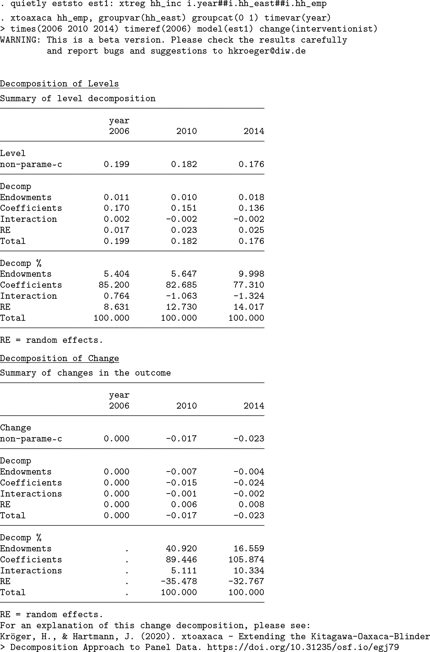
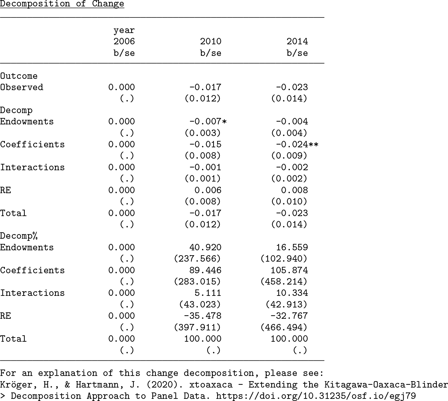
After fitting the model, we run the xtoaxaca command. In our example, we specify hh_emp as the decomposition variable we are interested in, the group variable (hh_east), and the two values of the group variable that we want to compare (0 and 1). Further, we need to specify the time variable (year) and the specific time values (2006 2010 2014), the reference time (2006), and the name of the stored fitted model. Finally, we tell xtoaxaca that we wish to use the interventionist approach, denoted by change(interventionist).

By default, xtoaxaca displays a table of the decomposition of levels and another table showing the decomposition of change. In the first table, the row non-parametric denotes the mean group differences in log household incomes as estimated nonparametrically from the observed data. The rows in the Decomp section show the results of the income gaps’ decomposition into an endowments part, a coefficient part, an interactions part, and a part that is due to the time-constant error term (RE). In our example, household compositions hardly contribute to the gap in household income, and their contribution grows only in 2014. Because the RE component is close to 0, our model is also reasonably well specified. However, the RE component is nonnegligible compared with the size of the other components. Further, we see that the decomposed parts sum up to the difference predicted by the base model for all years. The lower part of the table displays the relative contribution of the four decomposition effects to the overall gap.

The second table displays the results of the decomposition of change. We see the change in the income gap in comparison with the reference year 2006 in the second and third column. For the observed data, the gap decreased between 2006 and 2014 by 0.023 log incomes. We can now examine the role of changing endowments and coefficients over time. As we can see, the changing household composition decreased the gap by 0.004 log incomes, and the changing coefficients contributed 0.024 log incomes to the narrowing gap between 2006 and 2014. The part that is due to differences between groups in the time-constant error term increased the gap by 0.008 log incomes. While this part is rather small, it still indicates that group-specific panel dropout has a small effect on the results.

7.2 Bootstrapping for standard errors

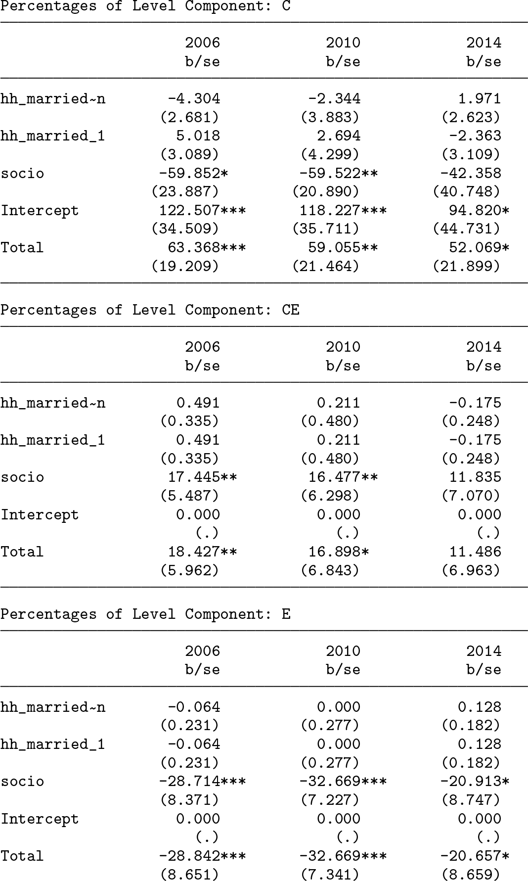
So far, we have decomposed the changes in household incomes between 2006 and 2014 in Germany and have the estimates but no standard errors. The xtoaxaca command provides a bootstrap() option to estimate the standard errors. Because there have been no attempts to analytically derive standard errors for all decomposition models of change over time, we believe that bootstrapping is a viable alternative. By default, xtoaxaca does not bootstrap the standard errors, because it is a potentially time-consuming endeavor.

Below, we see the same example as above with bootstrap standard errors. The point estimates of the decomposition components are by design identical to the previous example. However, we now get a standard error below the point estimate and can now be more confident that the households’ composition contributes about 5.4% to the income gap in 2006 and almost 10% in 2014, because the components are statistically significant. However, the size of the component of households’ changing composition is small in size and is not statistically significant.

7.3 Blocks of variables

One can also combine two or more variables to blocks and get the standard error via bootstrapping for their combined contribution to the decomposition of both levels and change. The relevant option is blocks(), and the resultsdata() option needs to be specified as well. Below is an example of code and output for variable blocks. The results for the variables are shown after all other output is given. Here the contribution of all categories of the variables hh_emp and hh_edu is combined into the block socio. The variable hh_married is treated separately. One can specify more than one block of variables.

7.4 Example 2—An intervention

As a further example, we simulate a dataset with a group variable (group), two time points, and two binary intervening variables, of which the first is exogenous (int1) and the second is endogenous to the first one (int2). The purpose of this example is to demonstrate how xtoaxaca can decompose change in group differences over time using multiple intervening and exogenous decomposition variables similar to experimental settings. For instance, an exogenous treatment effect, such as a policy change, could lead to increases in one group’s endowments, and we can then ask whether the treatment has any effect on the changing group differences.

As with the previous example, the first step involves fitting the model, which now includes two interaction terms: the interaction of the group variable with time and the first decomposition variable and the interaction of the group variable with time and the second decomposition variable. These two interaction terms are included so that the xtoaxaca command can estimate the groups’ counterfactual trajectories. In the second step, we call the xtoaxaca command followed by the two decomposition variables and specify the interventionist decomposition method (interventionist).

. use xtoaxaca_example2, clear

. quietly eststo m: xtreg dep i.time##i.group##i.int1 i.time##i.group##i.int2, > i(id)

As can be seen from the output, the changing endowments cause the gap to decrease by 4.5% over time, while the changing coefficients increase the gap by 105%. Thus, we conclude that the increasing gap between the groups over time is not caused by their changing endowments. On the contrary, they decrease the gap over time, while all the increase in the gap can be attributed to changing coefficients. If the role of the changing return to the decomposition variables is to be investigated, results using the detail option should be used (as illustrated in the last example in section 7.5) because the intercept is part of the coefficient block. A change in the intercept does not usually have a meaningful substantive interpretation with respect to the intervening variables and therefore might be considered an unexplained part within the coefficient component. Note also that because the example uses simulated data, the contribution of the time-constant error term is now exactly zero as expected by model assumptions.

7.5 Example 3—Interaction of decomposition variables

In the last example, we showed how a regression model has to be set up if interactions of decomposition variables are to be used in xtoaxaca. For this purpose, we distinguish between three types of interactions: Categorical-categorical, continuous-continuous, and categorical-continuous interactions.

Categorical-categorical interactions

For these kinds of interactions, we recommend generating a new variable that contains all combinations of the two categorical variables.

egen newvar = group(var1 var2)

Then, we can use this new variable (newvar) as a decomposition variable in both the regression and the xtoaxaca command.

Continuous-continuous interactions

For these kinds of interactions, the key is to create interaction terms by hand and then combine them with the standard Stata factor-variable notation of the group and time variable.

The first difference from the previous examples is the additional output that is generated by using the detail option. It provides not only the components of the decomposition but also the estimates for the endowments and coefficients for each variable and group. Note that for the interpretation of each variable and its contribution, separate assumptions about the reference category or value have to be made (see section 3.2 or Yun [2005]; Jann [2008]).

The second difference is that this example shows interactions of two continuous decomposition variables. If interactions of decomposition variables are used, note that the individual contribution of each interacted variable is now conditional on the value of the other variable. This means that in our example, we interacted experience with itself to get a squared term in the regression equation. The contribution of labor market experience (exp) now varies along the values of labor market experience.

For this particular example, we could state that the difference in change between groups A and B and time points 4 and 2 is explained about 20% by the difference in change in coefficients in the experience variable at the 15 years of experience in the sample (value of 0). If labor market experience is not centered at a meaningful value, this might not be a particular useful result.

Categorical-continuous interactions

The strategy described in section 7.5 for continuous-continuous interactions technically also works for categorical-continuous interactions. There are two limitations, however. First, normalization (3.2) for the categorical variable is not possible. This also implies that we cannot interpret the results for the decomposition by Kim (2010) as originally intended, because this decomposition relies on normalization. Second, we believe that it is overall very difficult to interpret the detailed output for such a decomposition. Users might consider performing the decomposition separately for the categorical variable they wish to interact with the continuous variable to ease interpretation.

8 Limitations

We focus on continuous outcomes and linear models but believe that the general approach can be generalized to nonlinear models as well, as it has been for the crosssectional KOB decomposition (Bauer and Sinning 2008; Jann 2008). Furthermore, applying regression with recentered influence functions in the modeling step might also be a way to circumvent the current restrictions to linear models of xtoaxaca (Essama-Nssah and Lambert 2012; Firpo, Fortin, and Lemieux 2018), as exemplified in the community-contributed command oaxaca_rif (Rios-Avila 2020).

Our decomposition approach is further limited to mean decompositions. Longitudinal decompositions of or using other distributional statistics (for example, percentiles, variances) might also be useful as user-friendly programs (Fortin, Lemieux, and Firpo 2011; Blau and Kahn 1992; Juhn, Murphy, and Pierce 1993).

9 Conclusion

We provided a systematic extension of the KOB decomposition to longitudinal (and multilevel) data. We reviewed five central approaches to the decomposition of change. We noted that none of them are directly useful for the evaluation of an intervention, policy changes, or natural experiments. We proposed an extension of the Wellington (1993) decomposition of change over time from an interventionist perspective. We introduced the xtoaxaca command, which implements the decomposition of levels and change (all six variants) over time in a user-friendly postestimation command for Stata. We are open to suggestions from users of xtoaxaca concerning new functions and other improvements so that we can update and improve it regularly.

11 Programs and supplemental materials

Supplemental Material, sj-zip-1-stj-10.1177_1536867X211025800 - Extending the Kitagawa–Oaxaca–Blinder decomposition approach to panel data

Supplemental Material, sj-zip-1-stj-10.1177_1536867X211025800 for Extending the Kitagawa–Oaxaca–Blinder decomposition approach to panel data by Hannes Kröger and Jörg Hartmann in The Stata Journal

Footnotes

10 Acknowledgments

We would like to thank Benita Combet and Christoph Halbmeier for helpful feedback on earlier versions of this article. We would also like to extend our special thanks to Benita Combet for extensive testing of earlier versions of xtoaxaca. All remaining mistakes remain, of course, the sole responsibility of the authors.

Hannes Kröger was funded by the Deutsche Forschungsgemeinschaft (DFG, German Science Foundation) 415809395, 427279591, 40965412 and the German Federal Ministry of Education and Research (BMBF, grants: 01UJ1911BY; 01NV1601B).

11 Programs and supplemental materials

To install a snapshot of the corresponding software files as they existed at the time of publication of this article, type

To install the current version of the software files, type

Notes

A Appendix

B Relations between change decompositions and KOB

In this section are the proofs that all decompositions of change presented in section 4 are derivatives of the difference between two KOB decomposition at two time points.¹⁰

Together, the four components fully decompose changes in group differences over time.

Proof.

As can be shown, WL1 and WL2 fully decompose changes in group differences over time.

Proof.

B.3 Interventionist

Finally, we can show that the three components added up to give the total difference in change between the two groups:

Proof.

Together, the components fully decompose the change in group differences over time.

Proof.

We can show that the KIM decomposition fully decomposes changes in group differences over time.

Proof.

References

Arrosa

M. L.

Gandelman

. 2016. Happiness decomposition: Female optimism. Journal of Happiness Studies 17: 731–756. https://doi.org/10.1007/s10902-015-9618-8.

Bauer

T. K.

Sinning

. 2008. An extension of the Blinder–Oaxaca decomposition to nonlinear models. Advances in Statistical Analysis 92: 197–206. https://doi.org/10.1007/s10182-008-0056-3.

Blau

F. D.

Kahn

L. M.

. 1992. The gender earnings gap: Learning from international comparisons. American Economic Review 82: 533–538.

Blau

F. D.

Kahn

L. M.

. 2017. The gender wage gap: Extent, trends, and explanations. Journal of Economic Literature 55: 789–865. https://doi.org/10.1257/jel.20160995.

Blinder

A. S.

1973. Wage discrimination: Reduced form and structural estimates. Journal of Human Resources 8: 436–455. https://doi.org/10.2307/144855.

DeLeire

2000. The wage and employment effects of the Americans with Disabilities Act. Journal of Human Resources 35: 693–715. https://doi.org/10.2307/146368.

Deming

W. E.

Stephan

F. F.

. 1940. On a least squares adjustment of a sampled frequency table when the expected marginal totals are known. Annals of Mathematical Statistics 11: 427–444. https://doi.org/10.1214/aoms/1177731829.

Essama-Nssah

Lambert

P. J.

. 2012. Influence functions for policy impact analysis. In Inequality, Mobility and Segregation: Essays in Honor of Jacques Silber, ed. Bishop

J. A.

Salas

, 135–159. Bingley, UK: Emerald.

Fairlie

R. W.

2005. An extension of the Blinder–Oaxaca decomposition technique to logit and probit models. Journal of Economic and Social Measurement 30: 305–316. https://doi.org/10.3233/JEM-2005-0259.

10.

Firebaugh

Warner

, and Massoglia

. 2013. Fixed effects, random effects, and hybrid models for causal analysis. In Handbook of Causal Analysis for Social Research, ed. Morgan

S. L

, 113–132. Dordrecht: Springer. https://doi.org/10.1007/978-94-007-6094-3_7.

11.

Firpo

S. P.

Fortin

N. M.

, and Lemieux

. 2018. Decomposing wage distributions using recentered influence function regressions. Econometrics 6: 28. https://doi.org/10.3390/econometrics6020028.

12.

Fortin

Lemieux

, and Firpo

. 2011. Decomposition methods in economics. In Handbook of Labor Economics, vol. 4A, ed. Ashenfelter

Card

, 1–102. Amsterdam: Elsevier.

13.

Freeman

R. B.

1980. Unionism and the dispersion of wages. ILR Review 34: 3–23. https://doi.org/10.1177/001979398003400101.

14.

Freeman

R. B.

1984. Longitudinal analyses of the effects of trade unions. Journal of Labor Economics 2: 1–26. https://doi.org/10.1086/298021.

15.

Goebel

Grabka

M. M.

Liebig

Kroh

Richter

Schröder

, and Schupp

. 2019. The German Socio-Economic Panel (SOEP). Journal of Economics and Statistics 239: 345–360. https://doi.org/10.1515/jbnst-2018-0022.

16.

Härdle

W. K.

Müller

Sperlich

, and Werwatz

. 2004. Nonparametric and Semiparametric Models. Berlin: Springer.

17.

Jann

. 2004. estout: Stata module to make regression tables. Statistical Software Components S439301, Department of Economics, Boston College. https://ideas.repec.org/c/boc/bocode/s439301.html.

18.

Jann

2008. The Blinder–Oaxaca decomposition for linear regression models. Stata Journal 8: 453–479. https://doi.org/10.1177/1536867X0800800401.

19.

Juhn

Murphy

K. M.

, and Pierce

. 1993. Wage inequality and the rise in returns to skill. Journal of Political Economy 101: 410–442. https://doi.org/10.1086/261881.

20.

Kalton

Flores-Cervantes

. 2003. Weighting methods. Journal of Official Statistics 19: 81–97.

21.

Kim

2010. Decomposing the change in the wage gap between white and black men over time, 1980–2005: An extension of the Blinder–Oaxaca decomposition method. Sociological Methods & Research 38: 619–651. https://doi.org/10.1177/0049124110366235.

22.

Kim

J. K.

Kim

J. J.

. 2007. Nonresponse weighting adjustment using estimated response probability. Canadian Journal of Statistics 35: 501–514. https://doi.org/10.1002/cjs.5550350403.

23.

Kitagawa

E. M.

1955. Components of a difference between two rates. Journal of the American Statistical Association 50: 1168–1194. https://doi.org/10.1080/01621459.1955.10501299.

24.

Liebig

Goebel

Richter

Schröder

Schupp

Kroh

Bartels

Erhardt

Fedorets

Franken

Giesselmann

Grabka

Krause

Kröger

Kühne

Metzing

Nebelin

Schacht

Schmelzer

Schmitt

Schnitzlein

Siegers

, and Wenzig

. 2018. Socio-Economic Panel (SOEP), data from 1984–2017, version 34.1. https://doi.org/10.5684/soep.v34.

25.

Machado

J. A. F.

Mata

. 2005. Counterfactual decomposition of changes in wage distributions using quantile regression. Journal of Applied Econometrics 20: 445–465. https://doi.org/10.1002/jae.788.

26.

Makepeace

Paci

Joshi

, and Dolton

. 1999. How unequally has equal pay progressed since the 1970s? A study of two British cohorts . Journal of Human Resources 34: 534–556. https://doi.org/10.2307/146379.

27.

Morgan

S. L.

Winship

. 2015. Counterfactuals and Causal Inference: Methods and Principles for Social Research. 2nd ed. New York: Cambridge University Press.

28.

Neuman

Oaxaca

R. L.

. 2003. Gender versus ethnic wage differentials among professionals: Evidence from Israel. Annales d’Économie et de Statistique 71 /72: 267–292. https://doi.org/10.2307/20079055.

29.

Oaxaca

1973. Male–female wage differentials in urban labor markets. International Economic Review 14: 693–709. https://doi.org/10.2307/2525981.

30.

Oaxaca

R. L.

Choe

. 2016. Wage decompositions using panel data sample selection correction. IZA Discussion Paper No. 10157, Institute of Labor Economics (IZA). http://ftp.iza.org/dp10157.pdf.

31.

Oaxaca

R. L.

Ransom

M. R.

. 1994. On discrimination and the decomposition of wage differentials. Journal of Econometrics 61: 5–21. https://doi.org/10.1016/0304-4076(94)90074-4.

32.

Rios-Avila

2020. Recentered influence functions (RIFs) in Stata: RIF regression and RIF decomposition. Stata Journal 20: 51–94. https://doi.org/10.1177/1536867X20909690.

33.

Smith

J. P.

Welch

F. R.

. 1989. Black economic progress after Myrdal. Journal of Economic Literature 27: 519–564.

34.

Taber

D. R.

Robinson

W. R.

Bleich

S. N.

, and Wang

Y. C.

. 2016. Deconstructing race and gender differences in adolescent obesity: Oaxaca–Blinder decomposition. Obesity 24: 719–726. https://doi.org/10.1002/oby.21369.

35.

Wellington

A. J.

1993. Changes in the male/female wage gap, 1976–1985. Journal of Human Resources 28: 383–411. https://doi.org/10.2307/146209.

36.

Winter

2002. survwgt: Stata module to create and manipulate survey weights. Statistical Software Components S427503, Department of Economics, Boston College. https://ideas.repec.org/c/boc/bocode/s427503.html.

37.

Yun

M.-S.

2005. A simple solution to the identification problem in detailed wage decompositions. Economic Inquiry 43: 766–772. With Erratum, Economic Inquiry 44: 198. https://doi.org/10.1093/ei/cbi053.

Supplementary Material

Please find the following supplemental material available below.

For Open Access articles published under a Creative Commons License, all supplemental material carries the same license as the article it is associated with.

For non-Open Access articles published, all supplemental material carries a non-exclusive license, and permission requests for re-use of supplemental material or any part of supplemental material shall be sent directly to the copyright owner as specified in the copyright notice associated with the article.

0.10 MB

0.00 MB