Sage Journals: Discover world-class research

Abstract

The proportion of explained variance is well defined in linear models, but Snijders and Bosker demonstrated that this concept is ill defined in linear multilevel models. Whenever a researcher adds a level 1 predictor to the model, the level 2 variance may increase because the level 2 variance also depends on the level 1 variance. This problem is more pronounced when there are few observations per cluster. The authors present a solution that allows researchers to decompose variance components from null models into parts explained and unexplained by level 1 predictors. The authors also offer an extension that incorporates level 2 predictors. This approach is based on multivariate multilevel modeling and provides a complete decomposition of the gross (or null model) variance components. The approach is also implemented in the user-written Stata program twolevelr2, and the online supplement contains worked code for implementation in R. The authors illustrate this method with an example analyzing sibling similarities in lifetime income.

Keywords

multilevel model random intercept model explained variance

The proportion of explained variance, often referred to as R², is a well-known concept in linear regression modeling and is extensively used in social science and beyond. One widely used way to obtain R² is to compare the proportional reduction in the variance of the error term before and after controlling for one or more predictor variables. In linear models, this approach is equivalent to applying the law of total variance to decompose the variance in the outcome into a part attributed to the model’s linear predictor and compare this with the total outcome variance including the variance of the error term. In linear multilevel models, however, the concept of explained variance is less clearly defined. According to a seminal article by Snijders and Bosker (1994), the before-after approach can yield negative R², something that is counterintuitive and inconsistent with the linear model case. Negative R² results from the variance of the level 2 errors increasing whenever we include a level 1 predictor in the observed or “fixed” part of the model.¹

Snijders and Bosker (1994) proposed to abandon the approach used in the conventional linear model in multilevel models and define explained variance in terms of the proportional reduction in prediction error. For level 2 variance components, this approach implies using the predicted group means before and after controlling for a predictor. This approach provides an easy way of obtaining an R² measure, but it does not constitute a decomposition of the underlying variance components of the null model. Moreover, Snijders and Bosker’s approach will lead to a poor approximation of the reduction in the underlying variance components whenever there are few observations per cluster (e.g., in panel data or sibling data).

In this article, we introduce a new approach to obtaining R² for the entire two-level model and for each level separately. The approach is based on multivariate multilevel modeling, which is a series of multilevel model equations for the outcomes and predictors for which level 1 and 2 errors are correlated across, but not within, equations (Baldwin et al. 2014; Goldstein 1995:89ff). It is conceptually similar to a seemingly unrelated regression approach in a multilevel framework. The multivariate models yield a variance-covariance matrix at levels 1 and 2, which can be used to back out appropriate R² statistics. We extend the framework to accommodate level 2 predictors, and we suggest a simple approach for dealing with models with a large number of level 1 covariates. Our approach is implemented in Stata with a freely available user-written program called twolevelr2 (Jann 2024). In the online supplement, we provide sample code that illustrates how the procedure can be implemented in R using the brms package (Bürkner 2017). As an example, we analyze the extent to which sister similarities in life cycle income can be explained by sibling similarities in schooling.

Why R² can be Negative

Snijders and Bosker (1994) demonstrated why R² can be negative in two-level models. Let Y_ij denote the outcome of observation i in cluster j, and let X_ij denote a corresponding predictor variable. Then we can write the two-level model excluding the predictor as

Y_{ij} = \tilde{α} + {\tilde{ω}}_{j} + {\tilde{ε}}_{ij},

(1)

where $\tilde{α}$ is the global mean in the outcome, ${\tilde{ω}}_{j}$ is the level 2 error, and ${\tilde{ε}}_{ij}$ is the level 1 error. The two-level model including the predictor can be written as

Y_{ij} = α + β X_{ij} + ω_{j} + ε_{ij},

(2)

where $β$ is the regression slope of the predictor variable.

Snijders and Bosker (1994) demonstrated that unexplained variance at level 2 can increase because the relationship between the variance of the level 2 error and the variance of the cluster means is given by

V ({\bar{Y}}_{. j}) = V ({\tilde{ω}}_{j}) + \frac{V ({\tilde{ε}}_{ij})}{n},

(3)

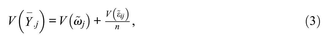
where n is the number of observations per cluster.² The intuition behind equation (3) is that $\bar{Y_{. j}}$ depends not only on the level 2 variance component but also the level 1 component penalized by the average number of observations per cluster. For each level 2 unit, there are n level 1 units, and thus the contribution to the level 2 variance from level 1 units is $\frac{V ({\tilde{ε}}_{ij})}{n}$ . Now imagine we control for a predictor variable without any level 2 variation; that is, X_ij contains only variation within and not between clusters. The variance of the cluster means will then remain unchanged,

V ({\bar{Y}}_{. j}) = V ({\bar{Y}}_{. j} | X_{ij}),

but, per equation (3), there will be an offsetting effect on the level 2 error variance, because the variance of the level 1 errors will decline; that is,

V ({\tilde{ε}}_{ij}) > V (ε_{ij}) .

The offsetting effect means that the level 2 error variance will increase; that is,

V ({\tilde{ω}}_{j}) < V (ω_{j}) .

In the more likely scenario in which X_ij contains variation at levels 1 and 2, the same offsetting effect will still be present because of the reduction of the variance in the level 1 errors, even though it may be counteracted by the reduction caused by the level 2 part of the predictor. Moreover, the offsetting effect will be particularly large whenever n is small, that is, when there are few observations per cluster, which is common in social science applications (e.g., in panel data or for number of siblings per family).

Snijders and Bosker (1994) suggested solving this problem by recasting explained variance in terms of the proportional reduction in prediction error. For the level 2 error, they suggested using the proportional reduction in the variance of the predicted cluster means by comparing $V ({\bar{Y}}_{. j})$ and $V ({\bar{Y}}_{. j} | X_{ij})$ , that is,

1 - \frac{V ({\bar{Y}}_{. j} - β {\bar{X}}_{. j})}{V ({\bar{Y}}_{. j})},

which amounts to aggregating to the cluster level and calculating the R² using the coefficient estimate $β$ from equation (2). This approach is elegant, but it does not measure the proportional reduction in the underlying or latent variance components. Moreover, it involves estimating two separate models, one without and one with the predictor variable.

A New Approach

We suggest using multivariate multilevel models to first obtain level 1 and level 2 variance-covariance matrices of both outcome and predictor variables and then use those variance-covariance matrices to back out relevant R² values. One advantage of our approach over existing approaches is that it relies on estimating only one model, a multivariate one. Moreover, in contrast to approaches that back out explained variance components by relying on the model including the predictor (Rights and Sterba 2019), our approach provides a decomposition of the variance in the null or empty model not involving any predictors, which often constitutes the explanandum in multilevel modeling (Snijders and Bosker 2012).

We first demonstrate this approach using the simplest setup possible, namely, the situation with one outcome variable, Y_ij, and one level 1 predictor variable, X_ij. We specify two two-level equations, one for each variable,

Y_{ij} = a^{Y} + u_{j}^{Y} + e_{ij}^{Y}

(4)

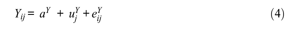
and

X_{ij} = a^{X} + u_{j}^{X} + e_{ij}^{X},

(5)

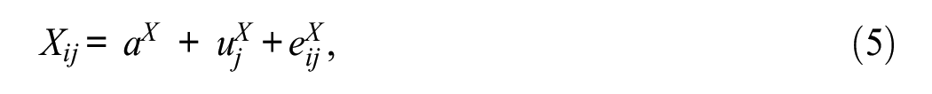
where a is the global intercept, u the level 2 error, and e is the level 1 error.³ The level 1 and level 2 errors are assumed to be independent of each other. The bivariate model is then given by the following variance-covariance matrices of the level 2 and level 1 errors, respectively,

Σ_{u} = [\begin{matrix} V (u_{j}^{Y}) & COV (u_{j}^{Y}, u_{j}^{X}) \\ COV (u_{j}^{Y}, u_{j}^{X}) & V (u_{j}^{X}) \end{matrix}]

(6)

Σ_{e} = [\begin{matrix} V (e_{ij}^{Y}) & COV (e_{ij}^{Y}, e_{ij}^{X}) \\ COV (e_{ij}^{Y}, e_{ij}^{X}) & V (e_{ij}^{X}) \end{matrix}] .

(7)

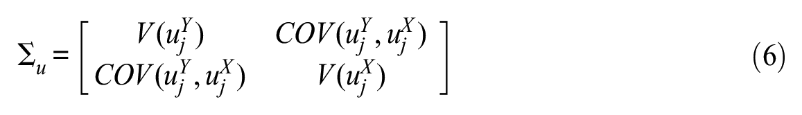
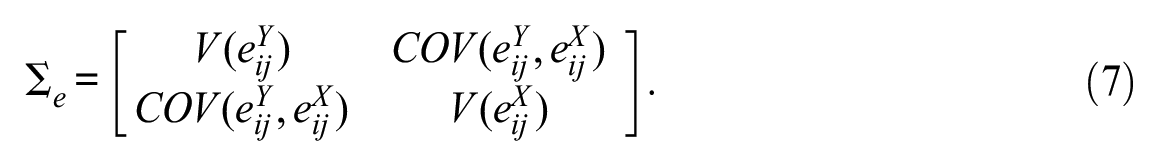
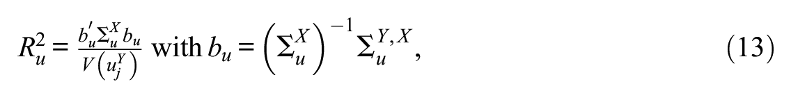
In this model, the level 1 and level 2 error terms are allowed to be correlated across (but not within) equations (4) and (5). The variance-covariance matrices contain all that is needed to obtain relevant measures of the proportion of explained variance. The proportional reduction in the variance of the level 2 error term is given by

R_{u}^{2} = \frac{b_{u}^{2} V (u_{j}^{X})}{V (u_{j}^{Y})},

(8)

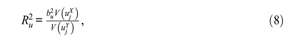
where

b_{u} = \frac{COV (u_{j}^{Y}, u_{j}^{X})}{V (u_{j}^{X})} .

The corresponding R² for level 1 is given by

R_{e}^{2} = \frac{b_{e}^{2} V (e_{ij}^{X})}{V (e_{ij}^{Y})},

(9)

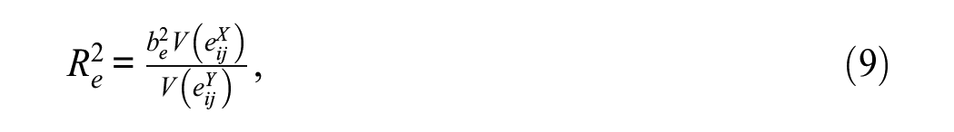
where

b_{e} = \frac{COV (e_{ij}^{Y}, e_{ij}^{X})}{V (e_{ij}^{X})} .

The total or global R² can then be defined as

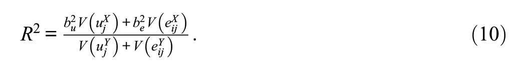
R^{2} = \frac{b_{u}^{2} V (u_{j}^{X}) + b_{e}^{2} V (e_{ij}^{X})}{V (u_{j}^{Y}) + V (e_{ij}^{Y})} .

(10)

It holds that $0 \leq R^{2} \leq 1$ , because when $COV (u_{j}^{Y}, u_{j}^{X}) = COV (e_{ij}^{Y}, e_{ij}^{X}) = 0$ , then $b_{u} = b_{e} = 0$ such that $R^{2} = 0$ . Furthermore, when X_ij fully explains level 2 and level 1 variance, $V (u_{j}^{Y}) = b_{u}^{2} V (u_{j}^{X})$ and $V (e_{ij}^{Y}) = b_{e}^{2} V (e_{ij}^{X})$ . It then follows that $R^{2} = 1$ .

Generalizing to Multiple Predictors

It is straightforward to generalize from the bivariate to the multivariate case. In this situation, we can “stack” the equations for the dependent variable and K level 1 predictors $X_{k, ij}$ ,

Y_{ij} = α^{Y} + u_{j}^{Y} + e_{ij}^{Y}

(11)

X_{k . ij} = α^{X_{k}} + u_{j}^{X_{k}} + e_{ij}^{X_{k}}, k = 1, \dots, K,

(12)

where $Σ_{u}$ and $Σ_{e}$ then denote the respective variance-covariance matrices of the level 2 and level 1 errors (see Goldstein 1995:89ff). From these matrices, it is straightforward to compute the variance of the linear predictor at each level and then plug these into the R² measures reported in the previous section. Specifically,

R_{u}^{2} = \frac{b_{u}^{'} Σ_{u}^{X} b_{u}}{V (u_{j}^{Y})} with b_{u} = {(Σ_{u}^{X})}^{- 1} Σ_{u}^{Y, X},

(13)

where $Σ_{u}^{X}$ is the submatrix of $Σ_{u}$ containing the variances and covariances of level 2 errors among predictors, and where $Σ_{u}^{Y, X}$ is the vector of covariances of level 2 errors between the dependent variable and the predictors. For level 1, the expressions are analogous. For convenience, we provide a user-written program, twolevelr2, in Stata that implements the approach (Jann 2024; see the online supplement for example code). In models with a large number of level 1 predictors, estimation may be computer intensive and lead to issues around numerical stability. To solve this issue, we suggest pairwise estimation of the entries in the variance-covariance matrices.⁴ The user-written Stata program implements both the pairwise and joint estimation approaches.

Including a Level 2 Predictor Variable

We have thus far considered explained variance when we include level 1 predictors that vary both within and between clusters (or, possibly, only within clusters). If we are interested in including level 2 predictors, that is, those that only vary between but not within clusters, then we have to extend our approach in the following way: relying on the Frisch-Waugh-Lovell theorem (Lovell 2008), we include these predictors directly in the multivariate multilevel equations, and then back out the explained part of the model using the law of total variance. We can do this because, per equation (3), there is no offsetting effect via the level 1 variance component, and thus we can obtain the proportional reduction in the level 2 variance component from including a level 2 predictor.

Assume we have a single level 2 predictor Z_j and a single level 1 predictor X_ij, then we can write the bivariate multilevel model as

Y_{ij} = a^{Y} + γ Z_{j} + u_{j}^{Y} + e_{ij}^{Y}

(14)

X_{ij} = a^{X} + θ Z_{j} + u_{j}^{X} + e_{ij}^{X}

(15)

and obtain the R² at level 2 as

R_{u}^{2} = \frac{γ^{2} V (Z_{j}) + b_{u}^{2} V (u_{j}^{X})}{γ^{2} V (Z_{j}) + V (u_{j}^{Y})},

(16)

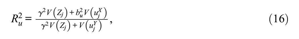
where

b_{u} = \frac{COV (u_{j}^{Y}, u_{j}^{X})}{V (u_{j}^{X})} .

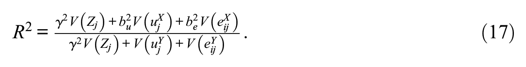
As Z_j does not vary within clusters, the level 1 R² remains unchanged. The global R² is given by

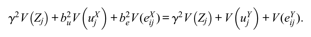
R^{2} = \frac{γ^{2} V (Z_{j}) + b_{u}^{2} V (u_{j}^{X}) + b_{e}^{2} V (e_{ij}^{X})}{γ^{2} V (Z_{j}) + V (u_{j}^{Y}) + V (e_{ij}^{Y})} .

(17)

This global R² is 0 when $γ = b_{u} = b_{e} = 0$ , and it is 1 when

γ^{2} V (Z_{j}) + b_{u}^{2} V (u_{j}^{X}) + b_{e}^{2} V (e_{ij}^{X}) = γ^{2} V (Z_{j}) + V (u_{j}^{Y}) + V (e_{ij}^{Y}) .

The generalization to multiple predictors at both levels is straightforward (with cross-level interaction terms to be treated as level 1 predictors).

Example

Social mobility scholars often use sibling data to obtain an estimate of the overall family background effect on a given labor market outcome of interest. To do so, researchers estimate a two-level random intercept model in which siblings are nested in families. The intraclass correlation from this model is a measure of the overall effect of family background because it captures the effects of everything siblings share, including their genetic makeup, common rearing environment, mutual interactions, and local neighborhoods (Solon 1999). Mobility scholars then often add sibling-specific variables, such as education, to see how much of the family-specific (or sibling group–specific) variance can be explained by education (Iannelli, Breen, and Duta 2024; Karlson and Birkelund 2024; Mazumder 2008).

We draw on sister data from the National Longitudinal Survey of Youth 1979 to examine the overall family background effect on lifetime income (Bureau of Labor Statistics 2019). In the National Longitudinal Survey of Youth 1979, we can identify sisters living in the same household at the time of the first interview and follow them through today. We are interested in evaluating the extent to which formal schooling (measured as highest grade completed at age 30) explains variation in income between (level 2) and within (level 1) families. We also investigate the extent to which parental income (a level 2 predictor) and sibling-specific formal schooling (a level 1 predictor) jointly explain the variance components. In a final example, we investigate how three level 1 predictors (schooling, cognitive ability, and educational aspirations) explain variance in income within and between families. Omitting singletons and sisters without valid information on the covariates and the dependent variable, our final sample includes 1,078 sisters from 502 sibling groups. Replication materials for this example are published along with this article.

Table 1 shows estimates of the bivariate multilevel model described in equations (4) and (5), in which sibling lifetime log income is the ultimate dependent variable. The first panel, log income, contains estimates of the model in equation (4), including the two variance components at level 1 (within families) and level 2 (between families); the second panel, schooling, contains the corresponding estimates in equation (5), that is, within- and between-family variation in schooling. The final panel contains the cross-equation covariances in the errors at each level. We use the estimated variances and covariances to back out the R² described earlier.

Table 1.

Estimated Intercepts, Variance Components, and Covariances in a Bivariate Multilevel Model of Sisters’ Schooling and Lifetime Income.

	Estimate	s.e.
Log income (y_ij)
Intercept	10.90	.03
Between-family variance (level 2)	.33	.04
Within-family variance (level 1)	.44	.03
Schooling (x_ij)
Intercept	13.18	.08
Between-family variance (level 2)	2.42	.23
Within-family variance (level 1)	2.27	.13
Covariances
Between families (level 2)	.58	.07
Within families (level 1)	.33	.04

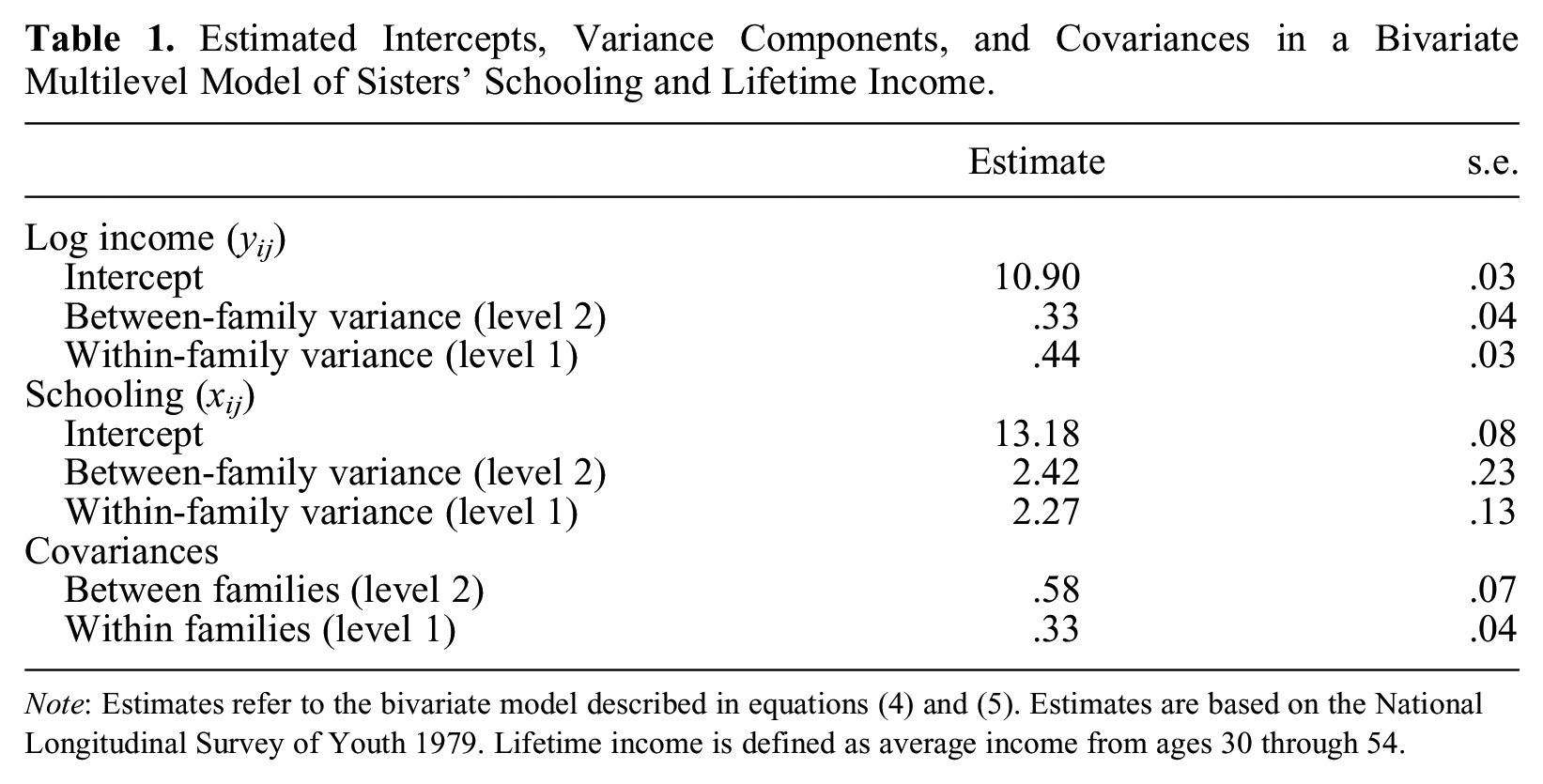
Note: Estimates refer to the bivariate model described in equations (4) and (5). Estimates are based on the National Longitudinal Survey of Youth 1979. Lifetime income is defined as average income from ages 30 through 54.

Table 2 shows the derived R² from the estimates as well as R² at level 2 computed from either the crude before-after approach⁵ or Snijders and Bosker’s (1994) approach. Using our new approach, we find that formal schooling accounts for about 42 percent of the total variance in log lifetime income between families, that is, at level 2. Had we instead used the crude before-after approach used in the existing literature, we would obtain a slightly smaller value of about 39 percent. This result is as expected: the before-after approach is affected by the offsetting term identified in Snijders and Bosker, leading to an attenuation of the R² at level 2. In column M1 in Table 2, we report the R² between families (at level 2) suggested by Snijders and Bosker. This estimate is only about 28 percent and thus substantially smaller than that based on our approach. This discrepancy arises because there are only a few observations (sisters) per cluster (family), so the cluster averages entering into the Snijders-Bosker R² are very crude proxies for the latent errors in the multilevel models.

Table 2.

Implied R² from Bivariate Models.

	M1	M2
R ² between families (level 2)	.420	.647
R ² within families (level 1)	.106	.105
Global R²	.241	.338
Snijders/Bosker R² between families (level 2)	.281	.431
Crude R² between families (level 2)	.393	.644

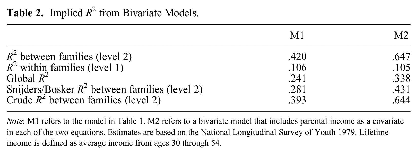
Note: M1 refers to the model in Table 1. M2 refers to a bivariate model that includes parental income as a covariate in each of the two equations. Estimates are based on the National Longitudinal Survey of Youth 1979. Lifetime income is defined as average income from ages 30 through 54.

Column M1 in Table 2 also shows that schooling explains about 11 percent of differences within families (at level 1), and the combined explanatory power of schooling on life cycle income is about 24 percent, a substantial portion. Column M2 in Table 2 reports the derived statistics from a bivariate model in which we include parental income (a pure level 2 predictor) as a covariate in each equation. The joint explanatory power between families (at level 2) then rises to about 65 percent, suggesting that parental income can incrementally account for about 23 percentage points over and above that accounted for by formal schooling, a nontrivial portion. As expected, we also find that R² within families (at level 1) is unchanged at 11 percent.⁶ In terms of overall explanatory power, formal schooling and parental income can account for about 34 percent of the total variance in lifetime income among sisters.

To show the utility of our approach when there are multiple level 1 predictors, in Table 3 we report derived R² from multivariate models that successively add level 1 covariates. The first row adds schooling, and estimates in that row are identical to those reported for M1 in Table 2. In the second row, we add cognitive ability and estimate a trivariate multilevel model. Adding cognitive ability increases the explained variance at level 2 to 68 percent, thus accounting for about 26 percent of the incrementally explained variance between families over and above that explained by education. The explained variance within families increases to 15 percent and the global R² to 37 percent. In the third and final row, we add educational aspirations and estimate a multivariate model with four equations. Adding educational aspirations does not lead to any incrementally explained variance.

Table 3.

Implied R² from Multivariate Models That Successively Add Level 1 Covariates.

	R ² between Families (Level 2)	R ² within Families (Level 1)	Global R²
+ Schooling	.420	.106	.241
+ Schooling + ability	.679	.148	.374
+ Schooling + ability + aspirations	.679	.151	.376

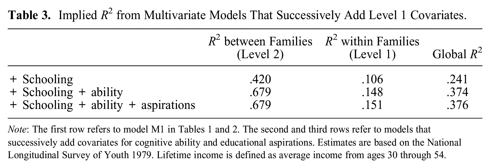
Note: The first row refers to model M1 in Tables 1 and 2. The second and third rows refer to models that successively add covariates for cognitive ability and educational aspirations. Estimates are based on the National Longitudinal Survey of Youth 1979. Lifetime income is defined as average income from ages 30 through 54.

Conclusion

We have presented a new way of obtaining the proportion of explained variance in two-level multilevel models. The approach solves a problem identified 30 years ago by Snijders and Bosker (1994). With our approach, researchers can decompose the variance components of the null model in a way equivalent to that used in conventional linear models. The approach is based on multivariate multilevel modeling and is therefore not affected by the offsetting effect at level 2 described in Snijders and Bosker (1994). The approach offers R² for levels 1 and 2 separately and jointly, and can easily be extended to accommodate level 2 predictors. We provide a tailor-made Stata routine (twolevelr2) for calculating the level 1 and 2 R² values, and in the supplementary materials to this article we provide code in R for reproducing our examples.

Footnotes

Funding

The authors disclosed receipt of the following financial support for the research, authorship, and/or publication of this article: For Kristian Bernt Karlson, the research leading to the results presented in this article received funding from the European Research Council under the European Union’s Horizon 2020 research and innovation program (grant agreement 851293).

ORCID iDs

Anders Holm

Ben Jann

Kristian Bernt Karlson

Data Note

Information about data access and all code necessary to replicate the results is provided at .

Supplemental Material

Supplemental material for this article is available online.

Notes

Author Biographies

Anders Holm is a professor of sociology at Western University in Canada and a research professor at the Rockwool Foundation. His research interests are quantitative methods and social inequality and stratification. He is currently involved in several large-scale research projects on the effects of vocational versus general education and peer effects in grade schools.

Ben Jann is a professor of sociology at the University of Bern in Switzerland. His research interests include social science methodology, statistics, social stratification, and labor market sociology. He is principal investigator of TREE, a large-scale, multicohort panel study in Switzerland on transitions from education to employment.

Kristian Bernt Karlson is a professor of sociology at the University of Copenhagen. He studies educational mobility, social stratification, and quantitative methods. He is the winner of the 2022 Raymond Boudon Award for early career achievement in sociology and the 2023 Leo Goodman Award for contributions to sociological methodology. He currently serves as deputy editor of Sociological Science. Recent work appears in the American Journal of Sociology, Sociological Methods & Research, and the European Sociological Review.

References

Anderson

Theodore W.

2003. An Introduction to Multivariate Statistical Analysis. 3rd ed. Hoboken, NJ: Wiley-Interscience.

Baldwin

Scott A.

Imel

Zac E.

Braithwaite

Scott R.

Atkins

David C.

2014. “Analyzing Multiple Outcomes in Clinical Research Using Multivariate Multilevel Models.” Journal of Consulting and Clinical Psychology 82(5):920–30.

Bureau of Labor Statistics. 2019. “National Longitudinal Survey of Youth 1979 Cohort, 1979–2016 (Rounds 1–27).”Columbus: Center for Human Resource Research, The Ohio State University.

Bürkner

Paul-Christian

. 2017. “brms: An R Package for Bayesian Multilevel Models Using Stan.” Journal of Statistical Software 80:1–28.

Goldstein

Harvey

. 1995. Multilevel Statistical Models. 2nd ed. London, UK: Arnold.

Iannelli

Cristina

Breen

Richard

Duta

Adriana

. 2024. “Following in the Parents’ Footsteps? Using Sibling Data to Analyse the Intergenerational Transmission of Social (Dis)advantage in Scotland.” European Sociological Review 40(3):390–402.

Jann

Ben

. 2024. “twolevelr2: Stata Module to Compute Within, Between, and Overall R-Squared in Linear Two-Level Models.” GitHub. Retrieved February 19, 2025. https://github.com/benjann/twolevelr2.

Karlson

Kristian B.

Birkelund

Jesper F.

2024. “Origins of Attainment: Do Brother Correlations in Occupational Status and Income Overlap?” European Sociological Review 40(3):379–89.

Lovell

Michael C.

2008. “A Simple Proof of the FWL Theorem.” Journal of Economic Education 39(1):88–91.

10.

Mazumder

Bhashkar

. 2008. “Sibling Similarities and Economic Inequality in the US.” Journal of Population Economics 21(3):685–701.

11.

Rabe-Hesketh

Sophia

Skrondal

Anders

. 2012. Multilevel and Longitudinal Modeling Using Stata. 3rd ed. College Station, TX: Stata Press.

12.

Raudenbush

Stephen W.

Bryk

Anthony S.

2002. Hierarchical Linear Models: Applications and Data Analysis Methods. 2nd ed. Thousand Oaks, CA: Sage.

13.

Rights

Jason D.

Sterba

Sonya K.

2019. “Quantifying Explained Variance in Multilevel Models: An Integrative Framework for Defining R-Squared Measures.” Psychological Methods 24(3):309–38.

14.

Snijders

Tom A. B.

Bosker

Roel J.

1994. “Modeled Variance in Two-Level Models.” Sociological Methods & Research 22(3):342–63.

15.

Snijders

Tom A. B.

Bosker

Roel J.

2012. Multilevel Analysis: An Introduction to Basic and Advanced Multilevel Modeling. Thousand Oaks, CA: Sage.

16.

Solon

Gary

. 1999. “Intergenerational Mobility in the Labor Market.” Pp. 1761–1800 in Handbook of Labor Economics, Vol. 3, Part A, edited by Aschenfelter

Card

Amsterdam, the Netherlands: Elsevier.

Explained Variance in Two-Level Models: A New Approach

Abstract

Keywords

Why R2 can be Negative

A New Approach

Generalizing to Multiple Predictors

Including a Level 2 Predictor Variable

Example

Conclusion

Footnotes

Funding

ORCID iDs

Data Note

Supplemental Material

Notes

Author Biographies

References

Why R² can be Negative