A Bayesian Semi-Parametric Approach for Modeling Memory Decay in Dynamic Social Networks

Abstract

In relational event networks, the tendency for actors to interact with each other depends greatly on the past interactions between the actors in a social network. Both the volume of past interactions and the time that has elapsed since the past interactions affect the actors’ decision-making to interact with other actors in the network. Recently occurred events may have a stronger influence on current interaction behavior than past events that occurred a long time ago–a phenomenon known as “memory decay”. Previous studies either predefined a short-run and long-run memory or fixed a parametric exponential memory decay using a predefined half-life period. In real-life relational event networks, however, it is generally unknown how the influence of past events fades as time goes by. For this reason, it is not recommendable to fix memory decay in an ad-hoc manner, but instead we should learn the shape of memory decay from the observed data. In this paper, a novel semi-parametric approach based on Bayesian Model Averaging is proposed for learning the shape of the memory decay without requiring any parametric assumptions. The method is applied to relational event history data among socio-political actors in India and a comparison with other relational event models based on predefined memory decays is provided.

Introduction

As a result of the growing automated collection of information, fine-grained longitudinal network data are increasingly available in many disciplines, such as sociology, psychology, and biology. These data have the potential to revolutionize our understanding about complex social network dynamics as we can learn how the past affects the future, how interaction behavior changes in continuous time, and how past social interactions lose their influence on the future away as time progresses. This has inspired social network scientists to develop network models that suit the inherent dynamic nature of these so-called relational event data. A relational event is defined as an action initiated by a sender and targeted to one or more receivers at a specific point in time. The relational event modeling framework aims to model the event rate: the speed at which relational events occur over a period of time between the actors in the model. The event rate can be expressed as a function of characteristics that quantify endogenous network patterns or exogenous characteristics that (jointly) determine how the network unfolds at some point in time (Butts, 2008). In sociological and psychological research, the application of these relational event models aims to find behavioral patterns and to shed light on the emergence of a global structure from network dynamics occurring at a local (typically, dyadic) level (Leenders, Contractor, and DeChurch et al., 2016; Schecter et al., 2018; Pilny et al., 2016).

Of particular interest is to understand what triggers actors to interact with each other. Actors might decide which mutual recipient to target their actions to depending on various aspects such as homophily, norms of reciprocity, the volume of past social interactions, triadic closure mechanisms, et cetera (Rivera, Soderstrom, and Uzzi, 2010). Past relational events influence future events in different ways. First, qualitative aspects of the past events play a role, such as whether the interaction was positive or a negative or who was the sender of the past event. For example, receiving a message from the company’s president might have a greater effect than getting a message from a regular colleague. Similarly, the valence of events may play a role: events with a negative connotation have been argued to have a greater effect than events with a positive connotation (Brass and Labianca, 1999; Labianca and Brass, 2006; Offer, 2021; Moerbeek and Need, 2003). Second, recent past events are generally expected to have a greater influence on the present than events that occurred a long time ago (Butts, 2008; Quintane et al., 2013; Brandes, Lerner, and Snijders, 2009; Mulder and Leenders, 2019). Having recently received praise from a colleague is likely to affect current interaction more than if that praise dates back a year ago.

While studies using relational event data tend to focus on the effects of endogenous statistics (e.g., to what extent actors repeat their past interactions, do they reciprocate interactions aimed at them, or do they prefer to interact with others with whom they share many other interaction partners with?) or exogenous statistics (e.g., does information sharing tend to go from lower-status actors to higher status actors, do friends share information at higher rates than non-friends, how much does co-location matter for communication in IT-enabled teams?), much less attention has been paid to exactly how long past events retain their influence on the present and future. This is the very subject of this paper. In particular, our aim is to derive a method that allows a researcher to empirically derive the shape of the function by which past events lose their influence on the future. This shape can be linear, exponentially decaying, or have any other shape. To unify our terminology, we will use the term “memory decay” for this phenomenon, even though we do not aim to model cognitive functions of the actors in the network. This terminology is not new. For example, Brandes, Lerner, and Snijders (2009) specify a half-life function that governs the decaying influence of events “motivated by the assumption that actors forget (or forgive)”. Similarly, Mulder and Leenders (2019) and Leenders, Contractor, and DeChurch et al. (2016) explicitly refer to this phenomenon as “memory decay.” Within the context of Temporal ERGM’s, Leifeld, Cranmer, and Desmarais et al. (2018) and Leifeld and Cranmer (2019) include so-called “memory terms” and allow the researcher to specify time-based functions (“time trends”) of how the time since a past tie affects the occurrence of later ties. Our focus is on the way the influence of past events on the future changes, that is akin to how long people “remember” (or care about) the past actively enough to still make it count towards the present and future. Because the effect of the past will almost always decrease as time passes, we will use the term “memory decay” throughout this paper to refer to the shape of the function that captures how the influence of a past event on future events changes as the time since the event increases.

Already in Butts (2008) seminal paper and the accompanying software (Butts, 2021), the importance of memory retention of past relational events is highlighted. So-called “participation shifts” were introduced that capture how the interaction dynamics shifts between dyads depending on the very last event that happened. These statistics assume that actors respond to the immediate past, regardless of what happened before that. In addition, a “recency” statistic is considered where the potential receivers for each potential sender are ordered based on their recent activity and a power-law is used to create a predictor variable (i.e., the reciprocal of the rank). This mechanism captures the extent to which actors take into account the last events they had with every other actor, discounting events from farther into the past. Finally, other endogenous statistics (such as inertia and reciprocity) are computed as the total volume of past interactions between actors and, hence, count all past events as equally important to the future and assume that no past event, however distant in the past, is ever forgotten. In sum, these statistics already capture three distinct ways in which the past is (dis)counted towards the present and the future and each reflect a different shape of memory decay.

More recently, other approaches have also been considered to better understand how (long) past activity affects future events. One approach has been to quantify a specific pattern of interactions according to specific predefined time intervals, such as a short-run expression (calculated by considering recently passed events) and a long-run expression (considering long-passed events in the computation) (Quintane et al., 2013; Quintane and Carnabuci, 2016; Perry and Wolfe, 2013; Kitts et al., 2017; Patison et al., 2015). The estimated effects for these intervals describe how different the impact of the specific pattern is on the event rate according to different recency of events constituting the pattern itself. Another approach consists of estimating the model while using a moving time window with a predefined fixed memory length with the result of a trend of the effects over the windows (Mulder and Leenders, 2019). An alternative to time-intervals-based methods weighs the influence of past events by an exponentially decreasing function with a given half-life parameter that describes the elapsed time beyond which the influence of an event in the calculation of the statistic is halved (Brandes, Lerner, and Snijders, 2009; Lerner, Bussman, Snijders, and Brandes et al., 2013; Leenders, Contractor, and DeChurch et al., 2016).

In all of these approaches, a researcher needs to predefine the memory lengths for the discretized model or predefine the steepness of the decay in the case of the continuous half-life model. Typically, heuristic considerations are used to specify this function. Notable exceptions include Brandenberger (2018) and Brandes, Lerner, and Snijders (2009) who explored the fit and robustness of the results by considering different choices for the half-life parameter. The question is, however, whether a prespecified memory decay appropriately captures the dependence between the time that has passed since the event and the current event. Depending on the context, certain decay shapes may be more suitable in terms of fit than other shapes. Model misfit may result in poor predictions and unreliable inferences.

Considering the dearth of time-sensitive theory to draw from (cf. Leenders, Contractor, and DeChurch et al. (2016); Ancona et al. (2001); Cronin, Weingart, and Todorova et al. (2011)), there is little theory (if any) to truly guide a researcher in the choice of an appropriate memory decay function for a research project at hand. Researchers have dealt with this by specifying choices for the decay function based on their experience with the empirical context or based on their own assumptions regarding the influence of time. Alternatively, an approach that we propose in this paper is to present a semi-parametric method for learning the actual shape of memory decay in relational event models. The method is semi-parametric in the sense that it does not make assumptions about a specific functional form for memory decay. Indeed, parameters that potentially govern the memory process and, in turn, determine its shape over time are often unknown and our intent is to minimize the challenge that is involved in prespecifying a memory function by a researcher. Our method can be used for finding any functional form of memory decay which could be an exponentially decreasing trend, a smoothed step-wise function, or other, possibly more (or less) complex, functional trends. Our semi-parametric method combines the relational event modeling framework (as in Butts (2008)) with Bayesian inference in the context of a model selection problem (Bayesian Model Averaging) (Volinsky et al., 1999). The idea is to consider a large “bag” of step-wise models with different interval configurations. Next, the fit is computed for all step-wise models, and subsequently, we model the shape as an average of these models weighted according to their respective fit to the observed data.

The paper is structured as follows. In next Section, we introduce the relational modeling framework along with the concept of memory decay. In A Step-Wise Memory Decay Model section, we formulate a step-wise memory decay model. In The Gradual Nature of Memory Decay section, we present a continuous memory decay model and highlight the potential use of step-wise models in approximating the continuous shape of the decay. In A Semi-Parametric Approach to Estimate a Smooth Memory Decay section, we present a semi-parametric method based on a Bayesian Model Averaging along with two weighting systems for generating random draws from the posterior memory decay. In Case Study: Investigating the Presence of Memory Decay in the Sequence of Demands sent Among Indian Socio-Political Actors section we apply the method to empirical data and we compare it to other models that predefine parametric memory decays. Concluding the paper, in Discussion section we discuss some considerations regarding the methodology and potential further development.

Relational event models that capture memory decay

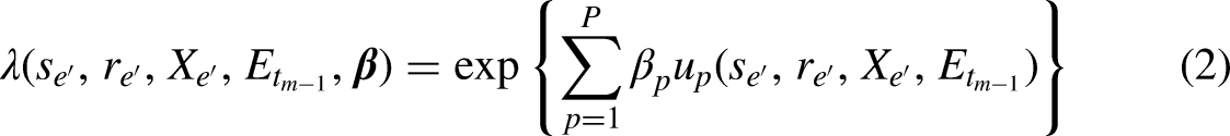
In the relational event framework (Butts, 2008), a relational event $e_m$ is characterized by the 3-tuple $(s_{e_m},r_{e_m},t_m)$ , respectively sender, receiver, and time of occurrence of the event. The joint probability of the realized ordered sequence of $M$ relational events, $E_{t_M}=(e_1,\dots ,e_M)$ , can be modeled as

$$p(E_{t_M};\mathit{\beta })=\prod _{m=1}^M[\lambda (s_{e_m},r_{e_m},X_{e_m},E_{t_{m-1}},\mathit{\beta })\prod _{e^{\prime }\in \mathcal{R}}^{}\exp \{-\lambda (s_{e^{\prime }},r_{e^{\prime }},X_{e^{\prime }},E_{t_{m-1}},\mathit{\beta })(t_m-t_{m-1})\}]$$

(1)

where $t_0$ (at $m=1$ ) is assumed to be equal to zero or to the starting time point of the case study. Further, $\lambda (s_{e_m},r_{e_m},X_{e_m},E_{t_{m-1}},\mathit{\beta })$ is the rate of the event $e_m$ occurred at time $t_m$ and $\lambda (s_{e^{\prime }},r_{e^{\prime }},X_{e^{\prime }},E_{t_{m-1}},\mathit{\beta })$ represents the event rate of any event $e^{\prime }$ that could have happened at time $t_m$ (including $e_m$ ). Indeed, $e^{\prime }$ belongs to the risk set $\mathcal{R}$ consisting of all sender/receiver combinations $\mathcal{S}\times R$ : where $\mathcal{S}$ and $R$ are, respectively, sets of all possible senders and receivers for the entire event sequence. If all actors can be senders as well as receivers in an interaction, then $\mathcal{S}\equiv R$ and the set of actors is simply referred to as $\mathcal{S}$ . Equation (1) can be viewed as the well-known survival model with time-varying covariates, where hazard and survival components form the likelihood in the same way (Lawless, 2002).

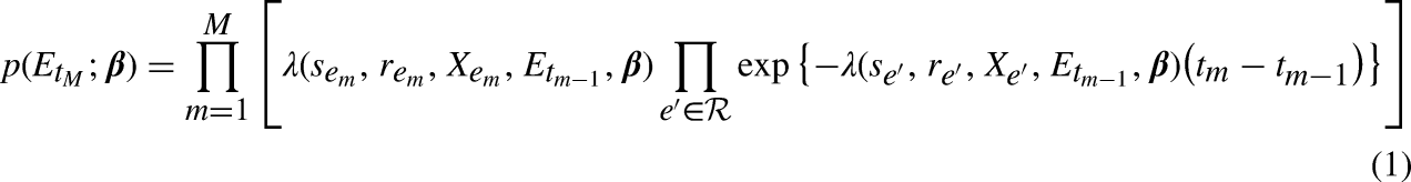
The rate of the specific dyadic event $e^{\prime }\in \mathcal{R}$ at a generic time $t_m$ is modeled as a log-linear function of statistics as follows

$$\lambda (s_{e^{\prime }},r_{e^{\prime }},X_{e^{\prime }},E_{t_{m-1}},\mathit{\beta })=\exp \left\{\sum _{p=1}^P{\beta }_p{u}_p(s_{e^{\prime }},r_{e^{\prime }},X_{e^{\prime }},E_{t_{m-1}})\right\}$$

(2)

where:

• ${\beta }_p$ with $p=1,\dots ,P$ , are parameters describing the effects of statistics on the logarithm of the event rate;

• $X_{e^{\prime }}$ is the set of covariates (exogenous attributes, possibly time-varying) associated with event $e^{\prime }$ ;

• $E_{t_{m-1}}$ refers to the collection of all of those events that occurred before $t_m$ ;

• $u_p(s_{e^{\prime }},r_{e^{\prime }},X_{e^{\prime }},E_{t_{m-1}})$ with $p=1,\dots ,P$ , are the statistics of interest and each one can depend either on transpired events (endogenous statistics calculated for all the dyads at each time point and given $E_{t_{m-1}}$ ) or on exogenous attributes ( $X_{e^{\prime }}$ ).

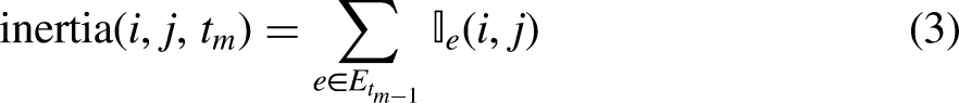
In the standard specification of the model, endogenous statistics describe patterns of interactions occurring in the network that are quantified at each time point by considering the whole history of events that happened from the initial state of the network (i.e., the first observed relational event) until the time point before the current one (i.e., $t_{m-1}$ in (2)). For instance, consider the standard formulation of the inertia statistic, which is a dyadic endogenous statistic that quantifies the volume of interactions of a specific dyad that occurred until the current time point. Inertia quantifies the extent to which specific relational events keep repeating over time. The corresponding formula at a generic time point $t_m$ with history $E_{t_{m-1}}$ is

$$\text{inertia}(\mathit{i}\mathit{,}\mathit{j}\mathit{,}{\mathit{t}}_{\mathit{m}}\mathit{)}\mathit{=}\sum _{\mathit{e}\in {\mathit{E}}_{{\mathit{t}}_{\mathit{m}\mathit{-}1}}}^{}{\mathbb{I}}_{\mathit{e}}\mathit{(}\mathit{i}\mathit{,}\mathit{j}\mathit{)}$$

(3)

where ${\mathbb{I}}_e(i,j)$ is the indicator variable that assumes value 1 if the event $e\in E_{t_{m-1}}$ has $s_e=i$ and $r_e=j$ , 0 otherwise. The event rate for any possible event $e^{\prime }\in \mathcal{R}$ at time $t_m$ with only the inertia in the linear predictor can be written as

$$\lambda (s_{e^{\prime }},r_{e^{\prime }},E_{t_{m-1}},\mathit{\beta })=\exp \{{\beta }_{\text{inertia}}\text{inertia}({\mathit{s}}_{{\mathit{e}}^{\prime }}\mathit{,}{\mathit{r}}_{{\mathit{e}}^{\prime }}\mathit{,}{\mathit{E}}_{{\mathit{t}}_{\mathit{m}\mathit{-}1}}\mathit{)}\}$$

(4)

A positive estimate for ${\beta }_{\text{inertia}}$ reflects that actors interact at higher rates with those actors who were often receivers of their past interactions. This is a sign of social routinization: what happened in the past is bound to be repeated over and over into the future.

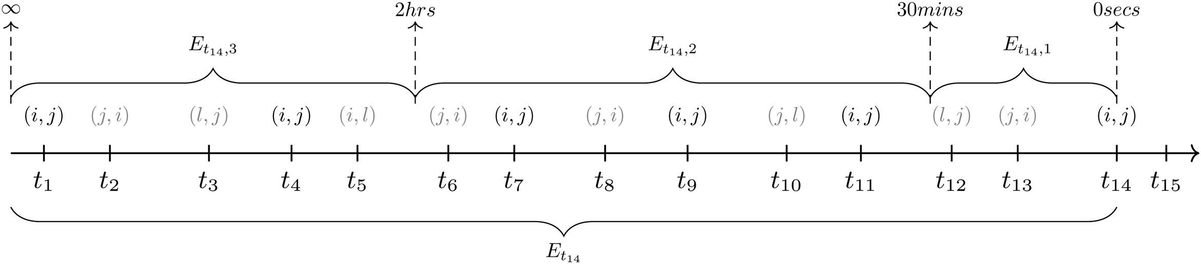
For instance, consider Figure 1 where a sequence of events from $t_1$ to $t_{14}$ is represented on a time line. In order to calculate the inertia at time $t_{15}$ for the specific dyad $(i,j)$ we need to count the number of past events in the history $E_{t_{14}}$ where $i$ targeted an action to $j$ , which is six in the example. Although this approach would give insights into how previous interactions between actors have influence on the event rate, we would be assuming long-passed events (such as those that happened 14 and 11 events ago, over two hours ago) to be equally influential as recent ones (such as the events that are only 1 or 4 events–or 45 minutes or so–old) in the computation of the statistics as well as on the event rate itself. This assumption may not be realistic for relational event data in practice as indicated earlier. Hence, our objective is to specify a model that is capable of accounting for this mutable effect of past events on the dyadic event rate.

Figure 1.

Example of the calculation of Inertia for the dyadic event $(i,j)$ , given the history of events $E_{t_{14}}=\{e_{t_1},\dots ,e_{t_{14}}\}$ .The event of interest in the calculation of the statistic is written in black, others are gray. Without considering intervals, the value of inertia at time $t_{15}$ is 6: the total count of $(i,j)$ events already occurred. When considering intervals (time bounds of each interval of the event history are highlighted by upwards arrows and labeled as $E_{t_{14},1}$ , $E_{t_{14},2}$ and $E_{t_{14},3}$ ), the value of inertia across the three intervals becomes ${\text{inertia}}_1(i,j,t_{15})=1$ , ${\text{inertia}}_2(i,j,t_{15})=3$ , and ${\text{inertia}}_3(i,j,t_{15})=2$ , where each one corresponds to the number of times that the event $(i,j)$ is observed within each interval.

A step-wise memory decay model

Step-wise decay for first-order endogenous effects

As a first step, we model the relative importance of past events as a function of the transpired time since the event was observed using a discretized, step-wise memory decay model (Perry and Wolfe, 2013). After the transpired time is divided into fixed intervals, endogenous statistics are computed for each interval and the corresponding endogenous effects are estimated. These effects quantify the relative importance of past events in predicting future events. For instance, considering the event sequence in Figure 1, we observe that at $t_{15}$ more than two hours have transpired since the starting time point and we divide the history of events $E_{t_{14}}$ into three sub-histories according to a set $\mathit{\gamma }$ of increasing time lengths, for example, $\mathit{\gamma }=(0secs,30mins,2hrs,\mathrm{\infty })$

$$\begin{array}{cc}& E_{t_{14},1}=\{e\in E_{t_{14}}:(t_{15}-t_e)\in (0secs,30mins]\}\\ & E_{t_{14},2}=\{e\in E_{t_{14}}:(t_{15}-t_e)\in (30mins,2hrs]\}\\ & E_{t_{14},3}=\{e\in E_{t_{14}}:(t_{15}-t_e)\in (2hrs,\mathrm{\infty })\}\end{array}$$

(5)

Where the first sub-history $E_{t_{14},1}$ contains all events transpired until 30 minutes before $t_{15}$ ; the second, $E_{t_{14},2}$ , includes those events happened between 30 minutes and 2 hours before $t_{15}$ ; lastly, the third sub-history, $E_{t_{14},3}$ , includes all events happened more than 2 hours before $t_{15}$ (the right bound is left undefined here). In Figure 1, the partition into sub-histories is shown by the upwards arrows corresponding to the time lengths $\gamma$ .

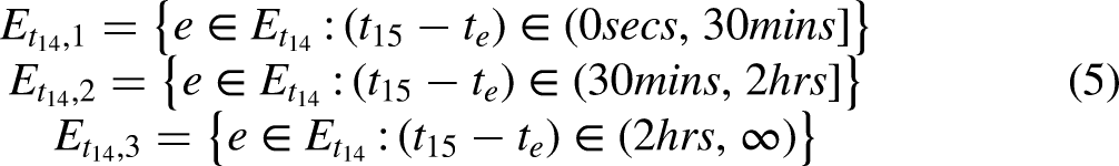
Therefore, three values of inertia can be calculated at any time point $t_m$ in the observed sequence by considering the three different partitions of the event history according to the increasing time lengths ( $\mathit{\gamma }$ ).

$${\text{inertia}}_k(\mathit{i}\mathit{,}\mathit{j}\mathit{,}{\mathit{t}}_{\mathit{m}}\mathit{)}\mathit{=}\sum _{\mathit{e}\in {\mathit{E}}_{{\mathit{t}}_{\mathit{m}\mathit{-}\mathit{1}}\mathit{,}\mathit{k}}}^{}{\mathbb{I}}_{\mathit{e}}\mathit{(}\mathit{i}\mathit{,}\mathit{j}\mathit{)}\mathit{\text{with}}\mathit{k}\mathit{=}\mathit{1}\mathit{,}\mathit{2}\mathit{,}\mathit{3}$$

(6)

Following the example in Figure 1, corresponding values of inertia according to intervals at time point $t_{15}$ are: ${\text{inertia}}_1(\mathit{i}\mathit{,}\mathit{j}\mathit{,}{\mathit{t}}_{15}\mathit{)}\mathit{=}1$ , ${\text{inertia}}_2(\mathit{i}\mathit{,}\mathit{j}\mathit{,}{\mathit{t}}_{15}\mathit{)}\mathit{=}3$ and ${\text{inertia}}_3(\mathit{i}\mathit{,}\mathit{j}\mathit{,}{\mathit{t}}_{15}\mathit{)}\mathit{=}2$ . We may expect that events that occurred in $E_{t_{14},1}$ have a larger impact on the event rate than those occurring in $E_{t_{14},2}$ and $E_{t_{14},3}$ . Although we do not make this assumption (as the goal is to learn from the data), the estimated effects relative to the three statistics will generally decrease in actual data, making the regression coefficient for inertia based on the most recent sub-history higher than that of inertia based on the most distant events, that is ${\beta }_{{\text{inertia}}_1}>{\beta }_{{\text{inertia}}_2}>{\beta }_{{\text{inertia}}_3}$ .

In a more general case where $K$ partitions of the current event history are defined according to increasing time lengths, such as

$$\mathit{\gamma }=({\gamma }_0,{\gamma }_1,\dots ,{\gamma }_K)\text{with}0={\gamma }_0<{\gamma }_1<\dots <{\gamma }_K=\mathrm{\infty }$$

(7)

we can partition the event history $E_{t_{m-1}}$ at time $t_m$ into subsets as

$$\begin{array}{cc}& E_{t_{m-1},1}=\{e\in E_{t_{m-1}}:{\gamma }_e(t_m)\in (0,{\gamma }_1]\}\\ & E_{t_{m-1},2}=\{e\in E_{t_{m-1}}:{\gamma }_e(t_m)\in ({\gamma }_1,{\gamma }_2]\}\\ & ⋮\\ & E_{t_{m-1},K}=\{e\in E_{t_{m-1}}:{\gamma }_e(t_m)\in ({\gamma }_{K-1},\mathrm{\infty })\}\end{array}$$

(8)

where ${\gamma }_e(t_m)=t_m-t_e$ represents the elapsed time at $t_m$ since the past event $e\in E_{t_{m-1}}$ . The general formula for inertia relative to the dyadic event $e$ with $(s_e=i,r_e=j)$ in the k-th partition of the $E_{t_{m-1}}$ at time $t_m$ is

$${\text{inertia}}_k(\mathit{i}\mathit{,}\mathit{j}\mathit{,}{\mathit{t}}_{\mathit{m}}\mathit{)}\mathit{=}\sum _{\mathit{e}\in {\mathit{E}}_{{\mathit{t}}_{\mathit{m}\mathit{-}\mathit{1}}\mathit{,}\mathit{k}}}^{}{\mathbb{I}}_{\mathit{e}}\mathit{(}\mathit{i}\mathit{,}\mathit{j}\mathit{)}\mathit{\text{with}}\mathit{k}\mathit{=}\mathit{1}\mathit{,}\dots \mathit{,}\mathit{K}$$

(9)

The event rate for any possible event $e^{\prime }\in \mathcal{R}$ at time $t_m$ where inertia is defined across $K$ partitions is

$$\lambda (s_{e^{\prime }},r_{e^{\prime }},E_{t_{m-1}},\mathit{\beta })=\exp \left\{\sum _{k=1}^K{\beta }_{{\text{inertia}}_k}{\text{inertia}}_{\mathit{k}}({\mathit{s}}_{{\mathit{e}}^{\prime }}\mathit{,}{\mathit{r}}_{{\mathit{e}}^{\prime }}\mathit{,}{\mathit{t}}_{\mathit{m}}\mathit{)}\right\}$$

(10)

Once statistics are calculated across the $K$ partitions, their corresponding parameters ${\beta }_{\text{inertia},\mathit{k}}$ , with $k=1,\dots ,K$ , can be estimated using the likelihood function in (1). In the interval case for the inertia, parameters express how the propensity of actors to target their actions to the same past receivers changes as a function of the recency of past events.

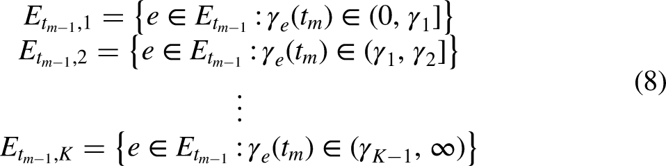
The use of interval statistics according to $K$ partitions of the event history directly relates to the dynamic of the estimated effects and their evolution will follow a step function as in Figure 2 with a mathematical function as in (11), that is based on the time lengths $\mathit{\gamma }$ used to create the partitions:

$${\beta }_{\text{inertia}}(\gamma )=\{\begin{array}{cc}{\beta }_{{\text{inertia}}_{\mathit{1}}}& \text{if }\gamma \in ({\gamma }_0,{\gamma }_1]\\ ⋮& \\ {\beta }_{{\text{inertia}}_{\mathit{K}}}& \text{if }\gamma \in ({\gamma }_{K-1},{\gamma }_K]\\ 0& \text{otherwise}\end{array}$$

(11)

Step-wise memory effects can also be modeled for other first-order endogenous statistics such as reciprocity, sender/receiver-in/out-degree whose formulas can be found in Appendix A.1.

Figure 2.

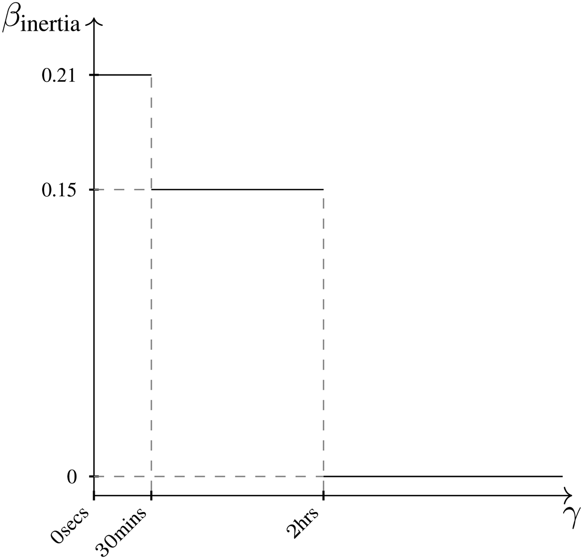
step-wise function for the effect of Inertia on the event rate. The function defines three intervals of the elapsed time $\gamma$ (on the x-axis): the first interval $\gamma \in (0\text{secs},30\text{mins}]$ , the second interval $\gamma \in (30\text{mins},2\text{hrs}]$ and the third interval $\gamma \in (2\text{hrs},\mathrm{\infty })$ . The y-axis shows the value of the effect ${\beta }_{\text{inertia}}$ for each interval.

Step-wise decay for higher order endogenous effects

Besides statistics that are based only on past interactions within a given dyad, the effects of higher order statistics involving more than two actors, can be used as well within this approach. Higher order endogenous statistics are characterized by more than one dyadic relational event in their formula. As such, the behavioral pattern of interest is more complex substantively as well as its computation. Indeed, in the case of triadic statistics, as with transitivity, the computation consists in the quantification of the number of times a dyad could potentially close a particular triangular structure if it occurred as next interaction after a specific sequence of past events.

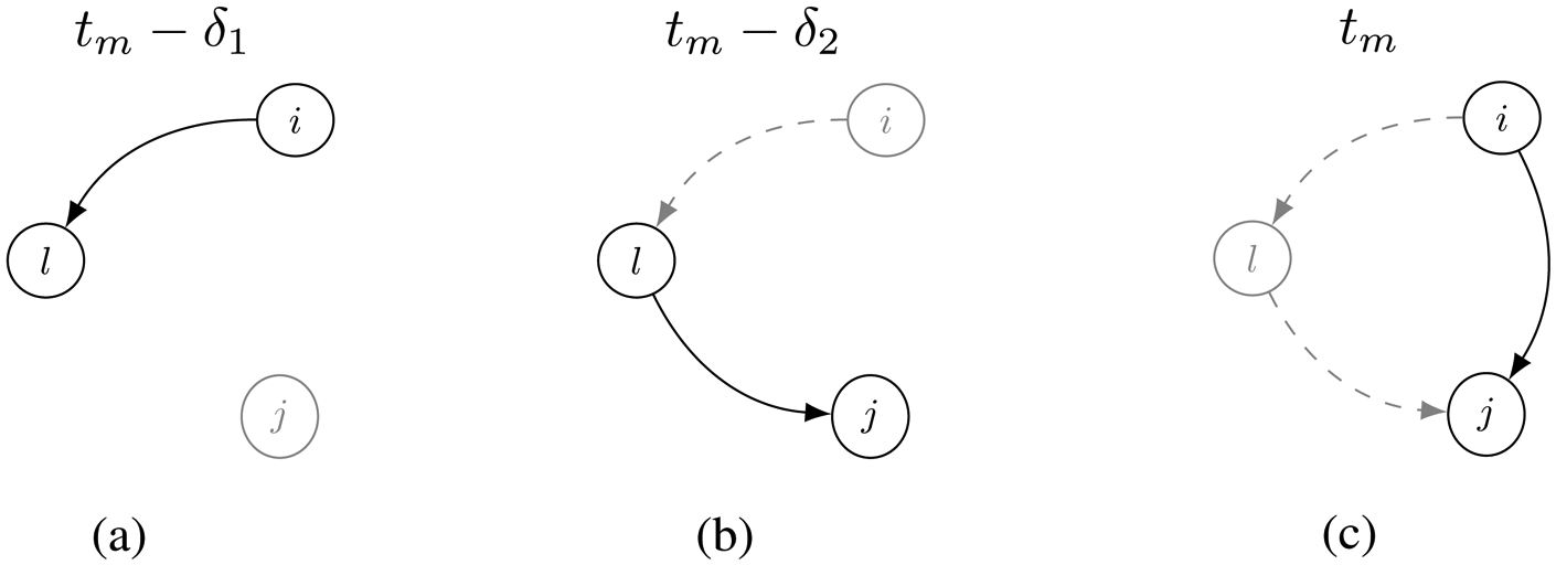
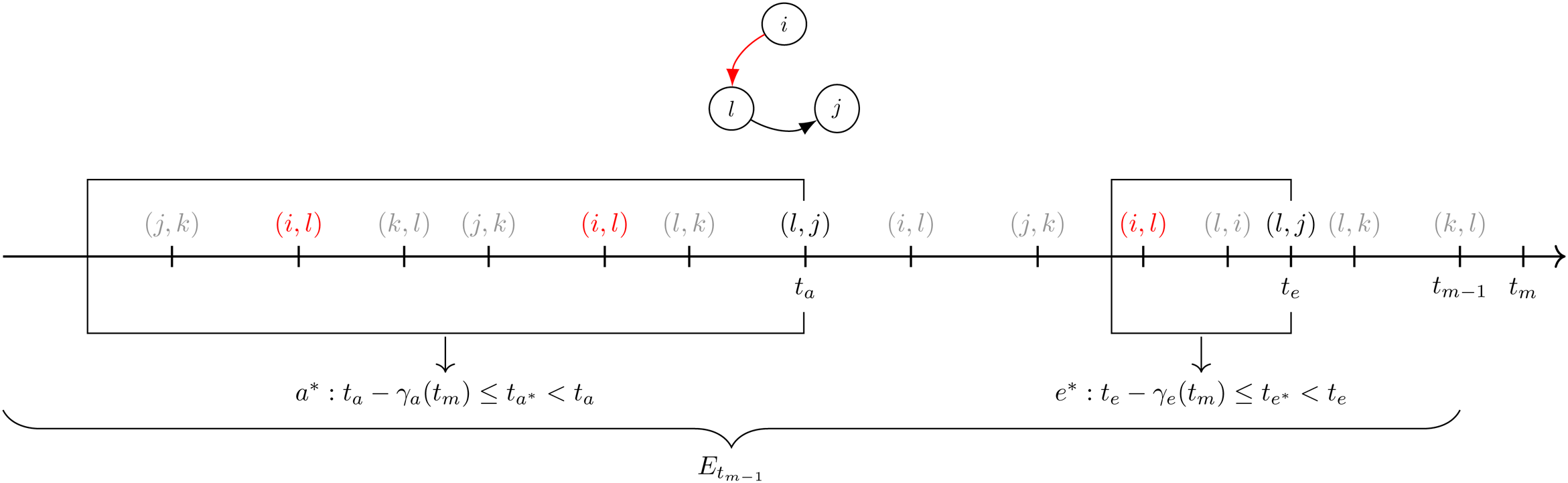
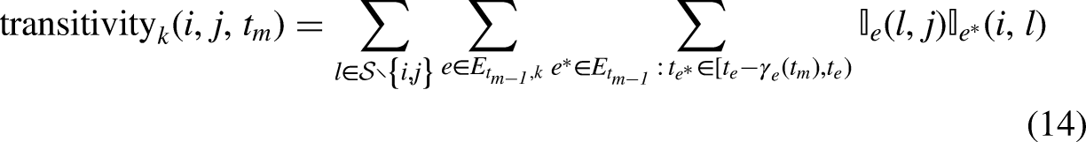
Figure 3 describes the pattern of the transitivity closure (Schecter et al., 2018) in the context of relational event data where interactions are time-ordered. The search for specific behavioral patterns can be improved by introducing such time-ordering in the calculation of the statistics. Specifically for transitivity closure, the following formula computes the statistic for the dyad $(i,j)$ at time $t_m$ :

$$\text{transitivity closure}(\mathit{i}\mathit{,}\mathit{j}\mathit{,}{\mathit{t}}_{\mathit{m}}\mathit{)}\mathit{=}\sum _{\mathit{l}\in \mathcal{S}\setminus \left\{\mathrm{i},\mathrm{j}\right\}}\sum _{\begin{array}{c}\mathrm{e}\in E_{t_{m-1}}\end{array}}\sum _{\begin{array}{c}{e}^{*}\in E_{t_{m-1}}:\\ t_{{\mathrm{e}}^{*}}\in [t_{\mathrm{e}}-{\gamma }_{\mathrm{e}}(t_{\mathrm{m}}),t_{\mathrm{e}})\end{array}}{\mathbb{I}}_{\mathit{e}}\mathit{(}\mathit{l}\mathit{,}\mathit{j}\mathit{)}{\mathbb{I}}_{{\mathit{e}}^{*}}\mathit{(}\mathit{i}\mathit{,}\mathit{l}\mathit{)}$$

(12)

where:

• ${\mathbb{I}}_e(l,j)$ is the indicator variable that assumes value 1 if the event $e\in E_{t_{m-1}}$ has $s_e=l$ and $r_e=j$ , and value 0 otherwise (the same reasoning applies to the other indicator variables in (12));

• $e$ and $e^{*}$ are any pair of events belonging to the event history $E_{t_{m-1}}$ such that $t_{e^{*}}<t_e$ ;

• ${\gamma }_e(t_m)=t_m-t_e$ is the time transpired at $t_m$ since the event $e\in E_{t_{m-1}}$ .

Figure 3.

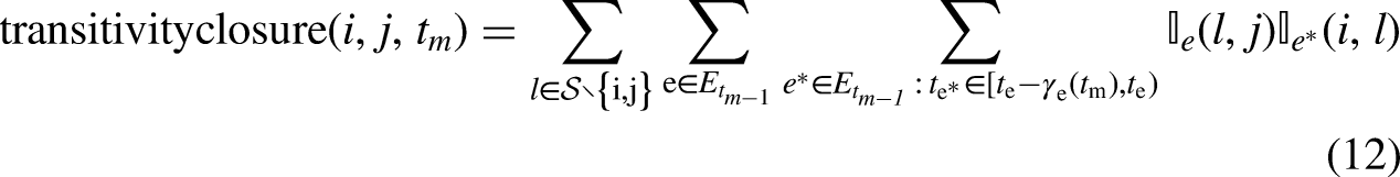
Figures from left to right describe the pattern of the transitivity closure in three time-framed steps. The time order of the three steps is described on the top of each graph, and it goes from the left, where the event $(i,l)$ opens the potential triad at $t_m-{\delta }_1$ , to the right, where the last event $(i,j)$ closes the triad at $t_m$ . Therefore, given the event history $E_{t_{m-1}}$ , the possible event $(i,j)$ occurring at $t_m$ (3c) can close a triad already opened with a third actor ( $l$ in the example) who acts as a broker in the process of information sharing/mediation. Events $(i,l)$ (3a) and $(l,j)$ (3b) occur by following the time order in the example, with ${\delta }_1$ and ${\delta }_2$ at time $t_m$ being the transpired times since the two events $(i,l)$ and $(l,j)$ , such that $t_m-{\delta }_1<t_m-{\delta }_2$ and $0\le {\delta }_2<{\delta }_1<t_m$ . Therefore, in this formulation the time order of the occurrence of events characterizing the triangular structure is taken into account. Gray nodes and dashed gray arrows indicate, respectively, inactive actors and events already occurred, whereas active actors and the occurring dyadic event are in black. (a) opening the triad: relational event $(i,l)\in E_{t_{m-1}}$ observed at time $t_m-{\delta }_1$ .; (b) information mediation stage operated by $l$ : relational event $(l,j)\in E_{t_{m-1}}$ observed at time $t_m-{\delta }_2$ . and (c) closing the triad: relational event $(i,j)$ that can potentially happen at time $t_m$ closing the triangular structure.

Figure 4 shows an example of the formula in (12) for just one $l\in \mathcal{S}\setminus \{i,j\}$ at time $t_m$ , with a history of events $E_{t_{m-1}}$ . In the example, two dyadic events $(l,j)$ , noted as $e$ and $a$ , occurred at $t_e$ and $t_a$ before $t_m$ . For each of them we seek backward for those events $e^{*}$ and $a^{*}$ that occurred within intervals based on the transpired time of $e$ ( ${\gamma }_e(t_m)=t_m-t_e$ ) and $a$ ( ${\gamma }_a(t_m)=t_m-t_a$ ) that are respectively $[t_e-{\gamma }_e(t_m),t_e)$ and $[t_a(t_m)-{\gamma }_a,t_a)$ . Hence, if any event $e^{*}$ or $a^{*}$ in these intervals has sender $i$ and receiver $l$ then the product of the two indicator variables in (12) will be one and so will be contribute to the sum, and is zero otherwise. In the specific example, as to event $a$ we observe two dyadic events $(i,l)$ that happened in $[t_a-{\gamma }_a(t_m),t_a)$ , whereas for $e$ we find just one event $(i,l)$ that occurred in $[t_e-{\gamma }_e(t_m),t_e)$ . Therefore, if the dyad $(i,j)$ is going to occur at $t_m$ it would close at least three potential triangular structures (of the type described in Figure 3) where the actor $l$ is the information mediator. The quantification in Figure 4 is just a simple example where the calculation of the transitivity is performed only in the case where the specific actor $l$ is the mediator (with $l$ being a different actor from $i$ and $j$ ). To quantify the transitivity closure for the dyad $(i,j)$ , which describes the total number of triangular structures closed by the occurrence of $(i,j)$ at $t_m$ , we have to sum all the potential triads that could be closed considering all the possible $N-2$ information mediators. This is described in formula (12) by the outer sum across all the actors in the network excluding $i$ and $j$ ( $\mathcal{S}\setminus \{i,j\}$ ) and indexed by $l$ . The new formula for transitivity closure accounts for the time order of events in the triadic behavioral pattern and assumes that those events $(i,l)$ happened earlier than an event $(l,j)$ and will count in the formula if and only if they transpired within the same time span of the specific $(l,j)$ .

Figure 4.

Example of the calculation of transitivity at $t_m$ for the dyad $(i,j)$ and information mediator $l$ : the event history $E_{t_{m-1}}$ counts only two events $(l,j)$ , at time $t_e$ and $t_a$ . In order to quantify the contribute of $l$ to the $\text{transitivity}(i,j,t_m)$ we : (i) find the second-last event in the pattern, that is $(l,j)$ , two in the example at $t_e$ and $t_a$ (in black); (ii) consider the backward intervals $[t_a-{\gamma }_a(t_m),t_a)$ and $[t_e-{\gamma }_e(t_m),t_e)]$ (black squares in the figure); (iii) for each interval quantify the number of $(i,l)$ observed (in red). In the example, the contribution of events $a$ and $e$ to the statistic is, respectively, 2 (because two events $(i,l)$ are observed in the backward interval of $t_a$ ) and 1 (because one event $(i,l)$ is observed in the backward interval of $t_e$ ). Thus, the value of transitivity for $(i,j)$ at $t_m$ with mediator $l$ is given by their sum, that is 3: if $(i,j)$ is the next event to occur it is going to close three potential triads where the information mediator was $l$ .

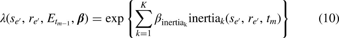
The event rate for any possible event $e^{\prime }\in \mathcal{R}$ at time $t_m$ with only the transitivity in the linear predictor is written as

$$\lambda (s_{e^{\prime }},r_{e^{\prime }},E_{t_{m-1}},\mathit{\beta })=\exp \{{\beta }_{\text{transitivity}}\text{transitivity}({\mathit{s}}_{{\mathit{e}}^{\prime }}\mathit{,}{\mathit{r}}_{{\mathit{e}}^{\prime }}\mathit{,}{\mathit{E}}_{{\mathit{t}}_{\mathit{m}\mathit{-}\mathit{1}}}\mathit{)}\}$$

(13)

A positive ${\beta }_{\text{transitivity}}$ means that the more partners $s_{e^{\prime }}$ and $r_{e^{\prime }}$ had in common in the past the more likely $s_{e^{\prime }}$ will choose $r_{e^{\prime }}$ as receiver of its next interaction. Vice versa, when ${\beta }_{\text{transitivity}}<0$ , the rate of the event $e^{\prime }$ lowers, meaning that there is a tendency by actors to discourage closure and thus to engage in fewer interactions with those actors they had shared a partner with. The statistic in (12) refers to the event history $E_{t_{m-1}}$ , that is the entire sequence of events since the onset until $t_{m-1}$ (including $e_{t_{m-1}}$ ). The ${\beta }_{\text{transitivity}}$ may depend on how recently the event $(l,j)$ occurred. Thus, transitivity can be redefined across intervals in the same way as inertia in previous section.

Consider the more general case of $K$ partitions of the current event history (as in (8)) according to $K+1$ increasing time lengths $\mathit{\gamma }$ (as in (7)). The transitivity as regards the $k\text{-th}$ interval, for the dyad $(i,j)$ at time $t_m$ will be,

$${\text{transitivity}}_{\mathit{k}}(\mathit{i}\mathit{,}\mathit{j}\mathit{,}{\mathit{t}}_{\mathit{m}}\mathit{)}\mathit{=}\sum _{\mathit{l}\in \mathcal{S}\setminus \{\mathit{i}\mathit{,}\mathit{j}\}}\sum _{\begin{array}{c}e\in E_{t_{m-1},k}\end{array}}\sum _{\begin{array}{c}{e}^{*}\in E_{t_{m-1}}:\\ t_{e^{*}}\in [t_e-{\gamma }_e(t_m),t_e)\end{array}}{\mathbb{I}}_{\mathit{e}}\mathit{(}\mathit{l}\mathit{,}\mathit{j}\mathit{)}{\mathbb{I}}_{{\mathit{e}}^{*}}\mathit{(}\mathit{i}\mathit{,}\mathit{l}\mathit{)}$$

(14)

where the quantification of potential triads is divided through the $K$ intervals of the history $E_{t_{m-1}}=\{E_{t_{m-1},1},\dots ,E_{t_{m-1},K}\}$ according to the time transpired at $t_m$ since the event $e$ , that is ${\gamma }_e(t_m)$ . However, the seeking of the event $e^{*}$ still considers the time interval as in (12). By using the interval formulation we are interested in understanding whether there exists an evolution of the transitivity effect on the event rate that depends on the recency of events constituting the triadic pattern. According to the step-wise formulation of transitivity, we can rewrite the rate in (13) as follows:

$$\lambda (s_{e^{\prime }},r_{e^{\prime }},E_{t_{m-1}},\mathit{\beta })=\exp \left\{\sum _{k=1}^K{\beta }_{{\text{transitivity}}_{\mathrm{k}}}{\text{transitivity}}_{\mathrm{k}}({\mathit{s}}_{{\mathit{e}}^{\prime }}\mathit{,}{\mathit{r}}_{{\mathit{e}}^{\prime }}\mathit{,}{\mathit{t}}_{\mathit{m}}\mathit{)}\right\}$$

(15)

The effect of transitivity across intervals conveys more information than in the case without intervals. Although, the interpretation of positive and negative effects remains the same (i.e. positive effects still promote the closure of triads as well as negative effects keep discouraging it), the intensity of such behaviors that promote/discourage triadic closure can change over time and this is the additional information we are after. For instance, if the effects from the first to the last interval are positive and decreasing, that is ${\beta }_{{\text{transitivity}}_{\mathit{1}}}>\dots >{\beta }_{{\text{transitivity}}_{\mathit{K}}}$ , this means that the closer in time the events in the triad are to each other the faster the third event in the pattern is likely to happen.

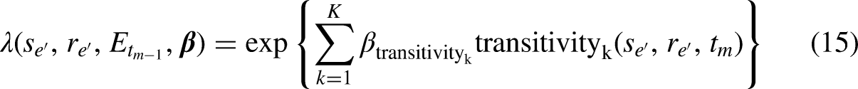
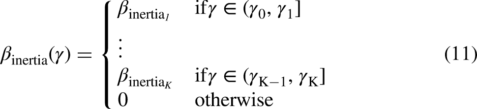
The function in (11) can be written also in the case of triadic statistics:

$${\beta }_{\text{transitivity}}(\gamma )=\{\begin{array}{cc}{\beta }_{{\text{transitivity}}_{\mathit{1}}}& \text{if }\gamma \in ({\gamma }_0,{\gamma }_1]\\ ⋮& \\ {\beta }_{{\text{transitivity}}_{\mathit{K}}}& \text{if }\gamma \in ({\gamma }_{K-1},{\gamma }_K]\\ 0& \text{otherwise}\end{array}$$

(16)

A simple example of step-wise effects for transitivity closure is shown in Figure 5: if we only consider transitivity closure in the model we can conclude that the more triadic events occurred recently, the sooner the third event in the triadic pattern is likely to happen. Formulas of further second-order statistics can be found in Appendix A.1.

Figure 5.

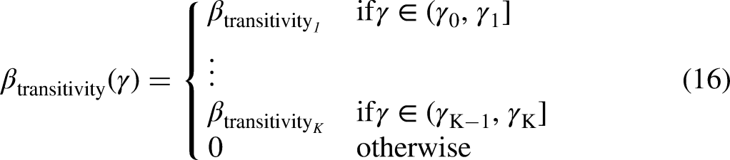
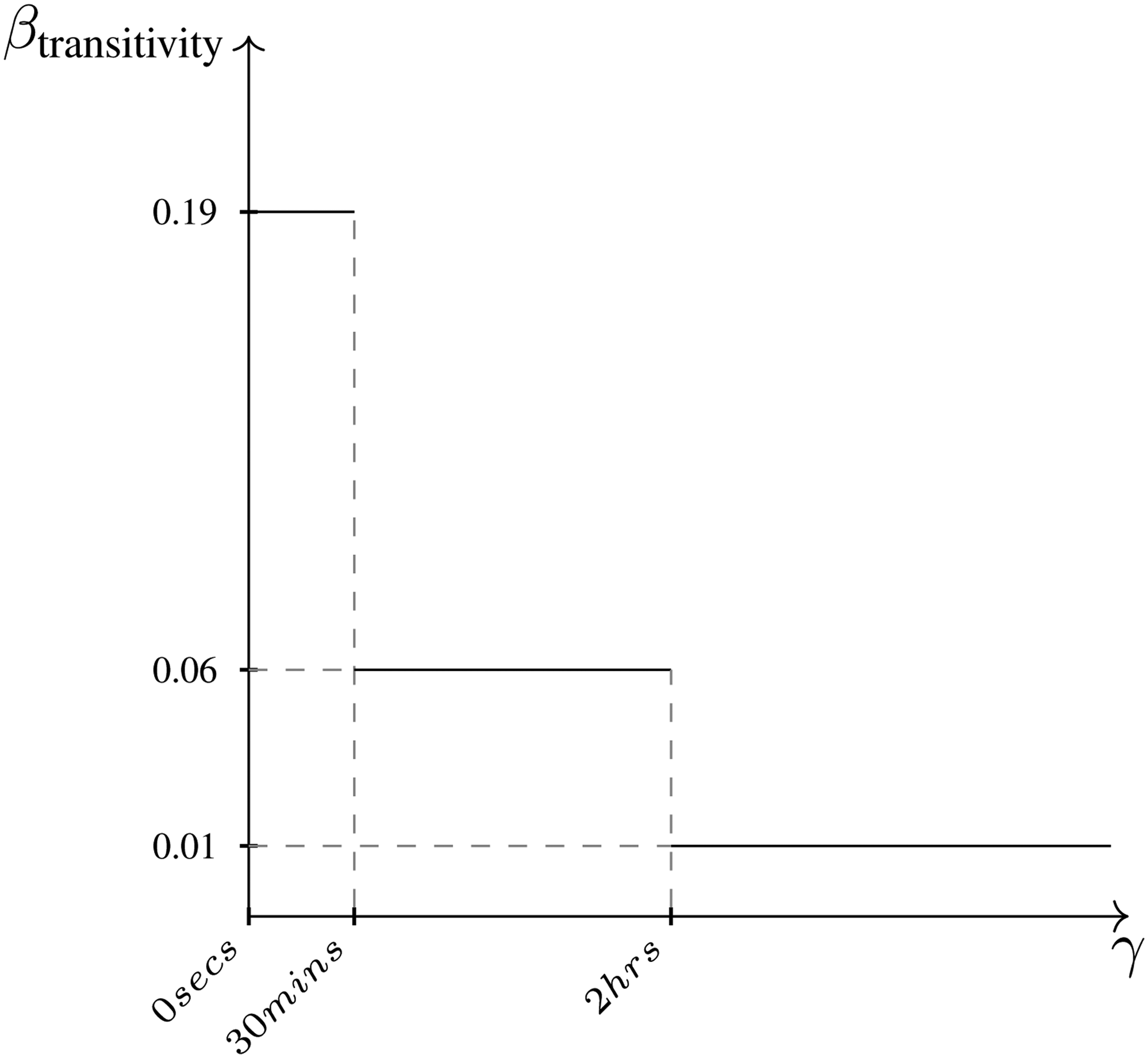
step-wise function for the effect of Transitivity on the event rate. The function defines three intervals of elapsed time $\gamma$ (on the x-axis): the first interval $\gamma \in (0\text{secs},30\text{mins}]$ , the second interval $\gamma \in (30\text{mins},2\text{hrs}]$ and the third interval $\gamma \in (2\text{hrs},\mathrm{\infty })$ . The y-axis shows the value of the effect ${\beta }_{\text{transitivity}}$ for each interval.

Estimation of a relational event model with a step-wise memory decay

The relational event model with step-wise memory decay of endogenous effects has the advantage that it can be easily estimated using existing software as relevent (Butts, 2008), goldfish (Stadtfeld and Hollway, 2020), rem (Brandenberger, 2018), or remverse (Mulder et al., 2020). This can be done as follows. First, the transpired time needs to be divided into disjoint intervals with bounds ${\gamma }_0,\dots ,{\gamma }_K$ . The bounds should be determined such that the step-wise function will be able to capture the expected memory; for periods where a fast (slow) decay is expected narrow (wide) intervals should be chosen. Next, each endogenous statistic (e.g., inertia, transitivity) is split in $K$ separate statistics that capture the volume of past interactions in the $K$ intervals of transpired time. The resulting set of relational event statistics can then be plugged into existing functions for fitting relational event models.

Despite the computational advantage, the step-wise memory decay in (11) and in (16) has two potential challenges: a substantive challenge is that may not always be realistic that memory decay occurs in a step-wise fashion in real life; a methodological challenge is that it may be unclear how many intervals ( $K$ ) should be chosen and where the boundaries $\mathit{\gamma }=({\gamma }_0,\dots ,{\gamma }_K)$ should be placed. When a researcher aims to learn a more fine-grained, potentially smoother continuous decay, it is of course possible to increase the number of intervals. However, we would still be constraining results to prespecified boundaries (the choice for which may not be obvious) and estimates could lose accuracy as this would greatly increase the number of free parameters in the model to be estimated and reduce the number of events per interval. Therefore, we now take the following two steps. First, we develop a continuous memory decay approach that solves these issues. Next, we show how the step-wise model can be used as a building block for an approximation of this continuous decay model.

The gradual nature of memory decay

Since past events often lose their effect gradually over time (rather than step-wise), we propose an often more realistic form of the memory decay in (11) and (16) where, instead of constraining effects to be constant within intervals of $\gamma$ , their change can be continuous over it and depends on a vector of parameters $\mathit{\theta }$ that define the resulting shape of the decay. The continuous effect for statistic $u$ can be written as

$${\beta }_u(\gamma ,\mathit{\theta })$$

(17)

where ${\beta }_u$ is a continuous function on $\gamma$ , describing the trend of the effect of $u$ such that ${\beta }_u:\mathcal{D}\to \mathbb{R}$ and $\mathcal{D}={\mathbb{R}}^{+}\setminus \{\gamma >{\gamma }_K\}$ , with ${\gamma }_K$ being a time length limit either due to the empirical data or simply justified by the researcher. The set of parameters $\mathit{\theta }\in S(\mathit{\theta })$ defines the shape of the decay, where $S(\mathit{\theta })$ is their support.

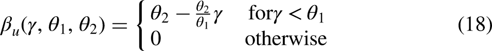
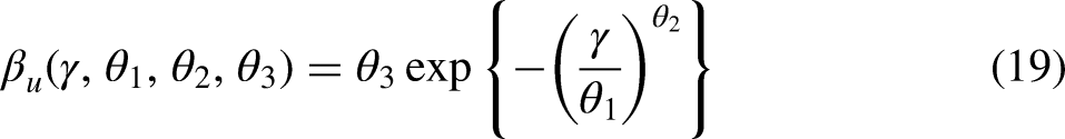
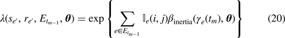
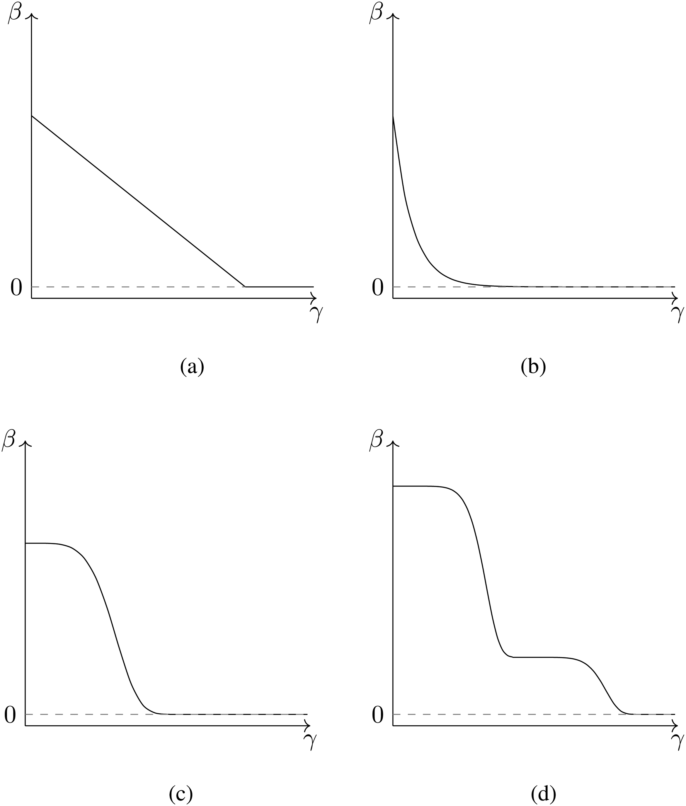
We propose several monotonously decreasing functions ${\beta }_u(\gamma ,\mathit{\theta })$ that might reflect the actual underlying memory decay.

The continuous trends in Figure 6 assume effects to be positive and decreasing towards zero as the time transpired since the event increases.

linear decrease (Figure 6a):

$${\beta }_u(\gamma ,{\theta }_1,{\theta }_2)=\{\begin{array}{cc}{\theta }_2-\frac{{\theta }_2}{{\theta }_1}\gamma & \text{,for }\gamma <{\theta }_1\\ 0& \text{otherwise}\end{array}$$

(18)

where $\mathit{\theta }=\{{\theta }_1,{\theta }_2\}$ , ${\theta }_2>0$ is the maximum value assumed by the function and $-\frac{{\theta }_2}{{\theta }_1}$ (with ${\theta }_1>0$ ) is the slope of the line that describes the steepness of the decrease;

exponential and one-smooth-step decrease (Figure 6b and Figure 6c):

$${\beta }_u(\gamma ,{\theta }_1,{\theta }_2,{\theta }_3)={\theta }_3\exp \{-{\left(\frac{\gamma }{{\theta }_1}\right)}^{{\theta }_2}\}$$

(19)

where the set of parameters $\mathit{\theta }=\{{\theta }_1,{\theta }_2,{\theta }_3\}$ consists of: ${\theta }_1>0$ and ${\theta }_3>0$ that are scale parameters ( ${\theta }_3$ corresponds to the maximum value assumed by the function), ${\theta }_2>0$ is a shape parameter. The survival function of a Weibull distribution is a specific case of the function (19) where the maximum value is ${\theta }_3=1$ . Moreover, where ${\theta }_2=1$ , ${\theta }_3=\frac{1}{{\theta }_1}$ , the (19) reduces to the exponential decreasing weight in Brandes, Lerner, and Snijders (2009) and the half-life parameter is then calculated as $T_{1/2}={\theta }_1\log 2$ . In most cases (except for the exponential one) the trend starts evolving at an initial constant value (one-smooth-step trend) that is the maximum value ${\theta }_3$ and then decreases to zero as $\gamma$ increases;

smoothed multiple steps (Figure 6d): this is a combination of two or more smoothed one-step trends.

The relative influence of past events on the dyadic event rate can follow other more complex shapes than those presented in Figure 6. As a result of this continuous definition of effects, inertia as well as other endogenous statistics are no longer computed as the accumulated number of past events but now consist of a sum of weights, where each weight changes according to the transpired time $\gamma$ of each event; this reflects the relative importance of past events updated at $t_m$ . Therefore, the event rate in (10) where only inertia effect is considered and inertia is divided in $K$ intervals becomes:

$$\lambda (s_{e^{\prime }},r_{e^{\prime }},E_{t_{m-1}},\mathit{\theta })=\exp \left\{\sum _{e\in E_{t_{m-1}}}^{}{\mathbb{I}}_e(i,j){\beta }_{\text{inertia}}({\gamma }_e(t_m),\mathit{\theta })\right\}$$

(20)

where $\beta ({\gamma }_e(t_m),\mathit{\theta })$ is a continuous function that returns the relative effect as to the event $e$ contributing to the inertia statistics, ${\gamma }_e(t_m)=t_m-t_e$ is the time transpired at $t_m$ since $t_e$ (and increases over time), and $\mathit{\theta }$ is the set of parameters that describe the shape of the decay. A formal mathematical procedure about moving from a step-wise effect function to a continuous effect function can be found in the Appendix A.2.

Figure 6.

Possible trends of the effect $\beta$ for any endogenous statistics. All four trends develop over $\gamma$ (x-axis), which is the elapsed time of the event characterizing the statistic. In these specific examples, trends decrease towards zero with different shapes depending on a set of memory parameters $\mathit{\theta }$ : (a) linear decay; (b) exponential decay; (c) one-smooth-step decay and (d) two-smooth-steps decay.

However, the process of estimation of the set of parameters $\mathit{\theta }$ governing the memory evolution results in a computationally complex maximization of the likelihood in (1). The more realistic scenario that the influence of past events changes as a continuous function of their elapsed time since the current time comes at the expense of constantly changing values of the network statistics; this increases the complexity of their estimation. Hence, in the next subsection we revalue the step-wise approach and present a Bayesian approach to approximate continuous memory decay with it.

A semi-parametric approach to estimate a smooth memory decay

In this section we propose a methodology that (i) builds on the computational advantage of the step-wise model introduced in Step-Wise Decay for Higher order Endogenous Effects section, (ii) avoids the issue of arbitrarily choosing intervals, and (iii) results in an approximate continuous estimate for memory decay. This is achieved by applying Bayesian Model Averaging (BMA) (Volinsky et al., 1999) to model memory decay in endogenous REM statistics. The idea is to randomly generate a bag of many step-wise models with different interval configurations for the transpired time. Next, the fit of all these models is evaluated and a weighted average of all step-wise models (weighted according to their relative fit) is achieved. This results in that approximate smooth trend for the memory decay that best fits the data.

We start with a simple example where we look at inertia. If we consider $Q$ step-wise models and denote a single step-wise model by ${\mathcal{M}}_q$ , then the Bayesian model average of the posterior distribution of the decay of the inertia effect ${\beta }_{\text{inertia}}$ as a function of the transpired time $\gamma$ is defined by

$$p({\beta }_{\text{inertia}}(\gamma )|E_{t_M})=\sum _{q=1}^{Q}p({\beta }_{\text{inertia}}(\gamma )|E_{t_M},{\mathcal{M}}_q)p({\mathcal{M}}_q|E_{t_M}).$$

(21)

Bayesian model averaging is, in fact, a direct application of the law of total probability where we marginalize over the discrete model space $\{{\mathcal{M}}_1,\dots ,{\mathcal{M}}_Q\}$ . Note that the law of total probability can be applied because a Bayesian framework allows us to quantify the uncertainty about a statistical model using probabilities. For other endogenous effects or other quantities of interest, Bayesian model averaging can be used in a similar manner. The posterior probabilities, $p({\mathcal{M}}_q|E_{t_M})$ , serve as relative weights in the Bayesian model average. Below, we consider two approaches to quantify these probabilities: BIC and WAIC. Before discussing these we explain how we can generate a bag of step-wise models to approximate different memory decay functions.

Generating a bag of step-wise relational event models

First, we define a bag of $Q$ step-wise relational event models where the transpired time is divided into interval configurations:

$${\mathcal{M}}_q:{\mathit{\gamma }}_q,\text{ with; }{\mathit{\gamma }}_q=({\gamma }_{q0},\dots ,{\gamma }_{q{K}_q}),$$

where $K_q$ denotes the number of intervals in model ${\mathcal{M}}_q$ . In order for the bag of models to approximate a variety of possible shapes, we vary both the number of intervals ( $K$ ) and the widths of the intervals. The sequences of time widths may be generated according to three features reflecting three possible changes of the decay over time:

• when memory change is likely to be stronger for the more recent events and to change less for events that already are in the farther past (where it is approximately constant) (e.g., an exponential decay), then intervals with increasing size will better catch this behavior and their widths will follow the inequality: ${\gamma }_k-{\gamma }_{k-1}<{\gamma }_{k+1}-{\gamma }_k$ for $k=1,\dots ,K-1$ . In other words, memory is short such that events are “forgotten” fairly fast and the most recent events carry a much higher weight than less recent events, and fairly distant events have as little effect on the future as events from the far past. The increasing size intervals (i) are generated by means of an algorithm based on the Dirichlet distribution and its pseudocode can be found in Appendix A.3.

• if the decay is expected to occur in the long term (close to ${\gamma }_K$ ) whereas it is steady during the more recent past (e.g., a one-smoothed step decay), then intervals with decreasing size will be best capable of catching this behavior and their widths will satisfy the inequality: ${\gamma }_k-{\gamma }_{k-1}>{\gamma }_{k+1}-{\gamma }_k$ for $k=1,\dots ,K-1$ . These widths can be generated by simply inverting the increasing widths in (i). This represents the situation where the effect of events decays only slowly for a while until they are far enough back in time, which is when they lose their effect fast (e.g., where events from the past week matter, but anything beyond that is quickly forgotten). The decreasing size intervals (ii) are generated by first drawing random intervals using increasing intervals according to (i), and subsequently, the order of the widths is inverted.

• if the decay is likely to decrease at a constant pace (e.g., a linear decreasing function), intervals of the same size will most easily emulate this behavior.

Figure 7 illustrates how different interval configurations can approximate different possible shapes. The figure also shows that a single step-wise model cannot approximate these smooth shapes accurately. Rather, an appropriate approximation can be achieved by taking a weighted average of many step-wise models. We discuss the computation of these weights next.

Figure 7.

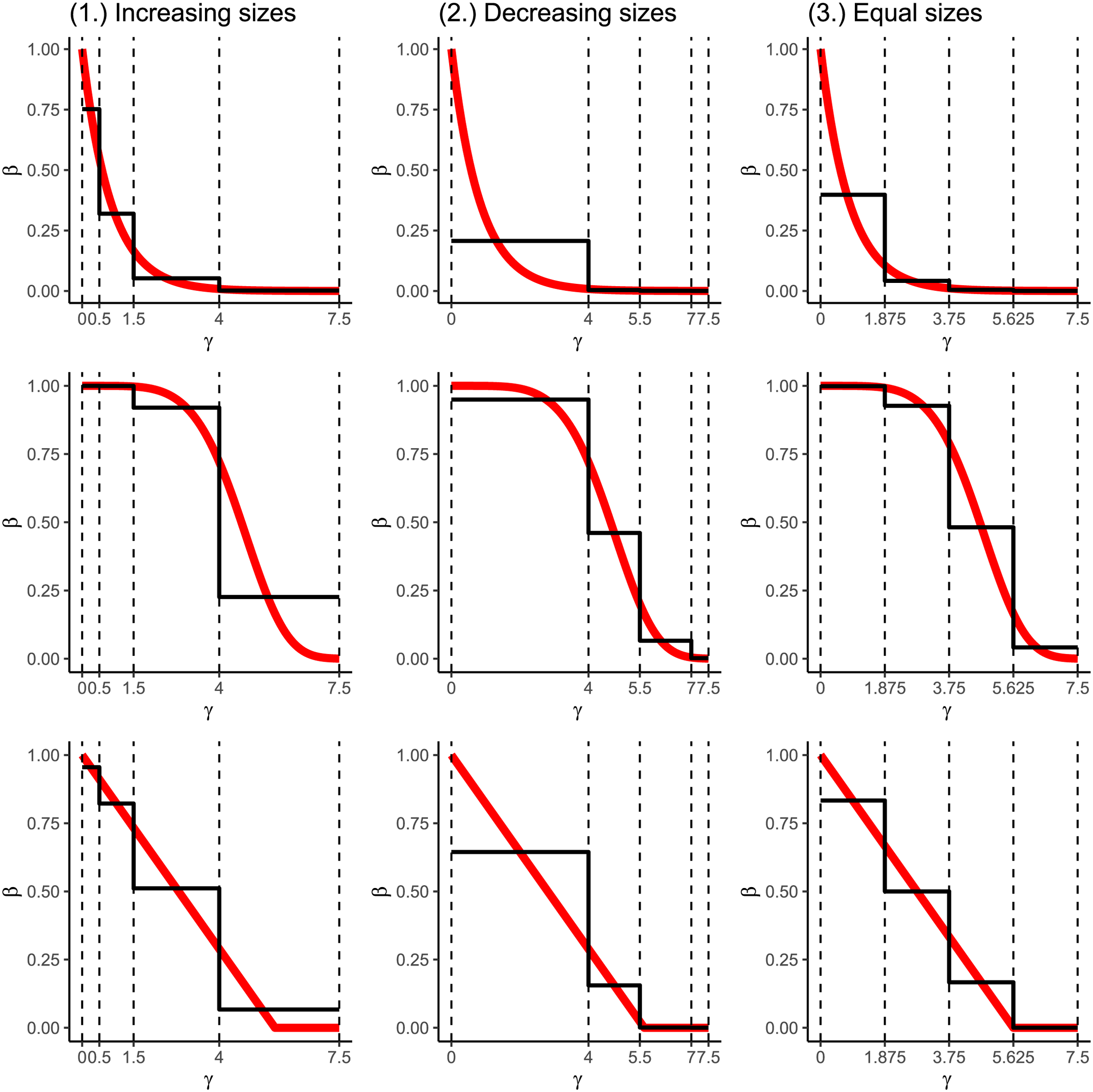
Examples of approximation of three different decays (red lines) by means of three types of step-wise functions (black lines) defined according to three different types of interval widths. The type of decay differs row-wise, from the top to the bottom: exponential decay, one-smooth-step decay and linear decay. The type of interval widths differs column-wise, from left to the right: increasing size, decreasing size and equal size intervals. The maximum time width is fixed to ${\gamma }_K=7.5$ .

Evaluating the fit of the step-wise relational event models

In this section, we describe two weighting systems for the $Q$ step-wise models that were generated in the previous section. The first weighting system is based on the BIC (capturing the probability of the observed data under each step-wise model (Schwarz, 1978; Raftery, 1995)). The second weighting system is based on the WAIC (which quantifies the predictive performance of each step-wise model (Watanabe, 2013; Vehtari, Gelman, and Gabry, 2017)).

BIC weights

In a Bayesian analysis, the posterior probability of a model is obtained using Bayes’ theorem:

$$p({\mathcal{M}}_q|E_{t_M})=\frac{p(E_{t_M}|{\mathcal{M}}_q)p({\mathcal{M}}_q)}{p(E_{t_M})},$$

where $p(E_{t_M}|{\mathcal{M}}_q)$ denotes the probability of the observed data under a given model (also referred to as the marginal likelihood), $p({\mathcal{M}}_q)$ is the prior probability of the model, and $p(E_{t_M})$ is the marginal probability of the data. We assume that all step-wise models are equally likely a priori, i.e., $p({\mathcal{M}}_q)=\frac{1}{Q}$ . The computation of the marginal likelihood can be expensive (Kass & Raftery, 1995). For this reason the Bayesian information criterion is used as an approximation (Schwarz, 1978; Raftery, 1995):

$$p(E_{t_M}|{\mathcal{M}}_q)\approx \exp \{-BI{C}_q/2\},$$

where the BIC of model $M_q$ is computed as

$$BI{C}_q=d_q\log (n)-2p(E_{t_M}|{\hat{\mathit{\beta }}}_q),$$

where $d_q$ is the number of parameters under model $M_q$ and $p(E_{t_M}|{\hat{\mathit{\beta }}}_q)$ is the maximized log likelihood under $M_q$ .

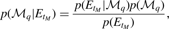
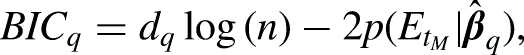
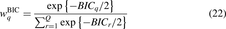
Thus, the normalized BIC weight for the $q\text{-th}$ model is

$$w_q^{\text{BIC}}=\frac{\exp \{-BI{C}_q/2\}}{\sum _{r=1}^Q\exp \{-BI{C}_r/2\}}$$

(22)

Despite its theoretical and computational appeal, it has been shown that the marginal likelihood, and its approximation via the BIC, may not perform well in Bayesian model averaging problems when the “true model” is not part of the bag of models that is considered. This is also called a $\mathcal{M}$ -open model selection problem (Yao et al., 2018). In the current setting this would be the case when the true decay function is smooth, that is not part of the bag of models but it could very well be the true shape of the decay in real-life networks. In this case, the relative weight in (22) converges to 1 for the step-wise model that is closest to the truth as the sample size grows. However, a smooth function can better be approximated by averaging over multiple step-wise models than by placing all its weight on one step-wise model. In such $\mathcal{M}$ -open problems it is preferable to use weights that are based on the WAIC.

WAIC weights

WAIC weights build upon the Expected Log-pointwise Predictive Density (ELPD) (Watanabe, 2013; Vehtari, Gelman, and Gabry, 2017; Yao et al., 2018). In each step-wise model, the ELPD quantifies the quality of the posterior predictions given the estimated posterior distribution of the model parameters. Therefore, if the model performs well in predicting new observations, then the predictive power quantified by the ELPD will assume a high value on a log-density scale as well as on a density scale. The calculation of the Watanabe-Akaike Information Criterion (WAIC) is based on an approximation of the ELPD as follows:

$${\widehat{elpd}}_q^{\text{waic}}={\widehat{lpd}}_q-{\hat{p}}_q^{\text{waic}}\text{,for}q=1,\dots ,Q$$

(23)

where the Log-pointwise Predictive Density ( ${\widehat{lpd}}_q$ ) represents the predictive log-density calculated on in-sample observations and typically overestimates the actual ELPD. This can be corrected by subtracting ${\hat{p}}_q^{\text{waic}}$ , which quantifies the uncertainty introduced by the posterior distribution of the model parameters ( ${\mathit{\beta }}_q$ ) in predicting the in-sample observations and can be seen as a form of penalization.

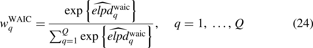
Hence, WAIC weights are computed as

$$w_q^{\text{WAIC}}=\frac{\exp \left\{{\widehat{elpd}}_q^{\text{waic}}\right\}}{\sum _{q=1}^Q\exp \left\{{\widehat{elpd}}_q^{\text{waic}}\right\}},q=1,\dots ,Q$$

(24)

Thus, the higher the estimated predictive power of a model ( ${\widehat{elpd}}_q^{\text{waic}}$ ), the higher its WAIC-based weight ( $w_q^{\text{WAIC}}$ ).

Bayesian model averaging for approximating smooth decay functions

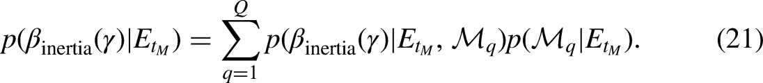
By means of BMA one can elicit a posterior estimate of a quantity of interest as well as its average posterior predictive distribution by finding the optimal linear combination of a set of models, and accounting, in turn, for their uncertainty. A crucial aspect of BMA is the use of model weights that quantify the relative importance of the models according to their posterior probability. In subsection BIC weights and WAIC weights we considered two weighting systems that can be employed in the estimation of the memory decay trend. Here we explain how to get posterior draws of the decay function of an endogenous effect from the Bayesian model averaged posterior.

In BMA, the posterior estimate of any parameter of interest can be calculated as the weighted mean of the posterior estimates provided by each model in the averaging. Considering (21), we can generate a posterior draw by first randomly selecting a model from the bag of models according to their relative weights, and then generate a trend from the posterior distribution of the selected model. We achieve this last step by approximating the posterior of $\mathit{\beta }$ using a multivariate normal distribution where the mean is equal to the maximum likelihood estimates and the posterior covariance matrix is set equal to the error covariance matrix. This is an application of large sample theory in a Bayesian framework (Gelman et al., 2013). We consider the following steps to get posterior draws:

Draw a model from ${\mathcal{M}}_q|E_{t_M}\sim \text{Multinomial}(\mathit{w})$ , where the vector of normalized weights $\mathit{w}=(w_1,\dots ,w_Q)$ quantifies the relative fit of the respective step-wise models;

Generate a vector of posterior effects from $\mathit{\beta }|{\mathcal{M}}_q,E_{t_M}\sim MVN({\hat{\mathit{\beta }}}_q,{\hat{\mathbf{\Sigma }}}_q)$ . The posterior distribution for the step-wise model $M_q$ (the model drawn at the first step) is approximated by a multivariate normal distribution with parameters given by maximum likelihood estimates under model $M_q$ and corresponding error covariance matrix;

Repeat steps 1 and 2 a sufficient number of times.

After these three steps, the resulting posterior distribution of each endogenous effect $\beta$ over $\gamma$ resembles Figure 8a. Then, we estimate the posterior decay of the effect over $\gamma$ as follows: (i) define a (dense) grid with evenly spaced $\gamma \in [0,{\gamma }_K]$ , where ${\gamma }_K$ is usually based on the data (Figure 8b, first step); (ii) for each $\gamma$ select the corresponding interval effect in each posterior draw (as shown by the step-wise functions in (11) and (16)), this selection results in a posterior density at a given $\gamma$ (Figure 8c, second step); (iii) calculate the posterior mode of these densities as well as their highest posterior density intervals at each $\gamma$ , resulting in a semi-continuous effect decay (Figure 8d). As a consequence of this, the posterior estimate of those statistics that are not defined in intervals (e.g, a baseline effect) is simply obtained with the draws generated after the three initial steps.

Figure 8.

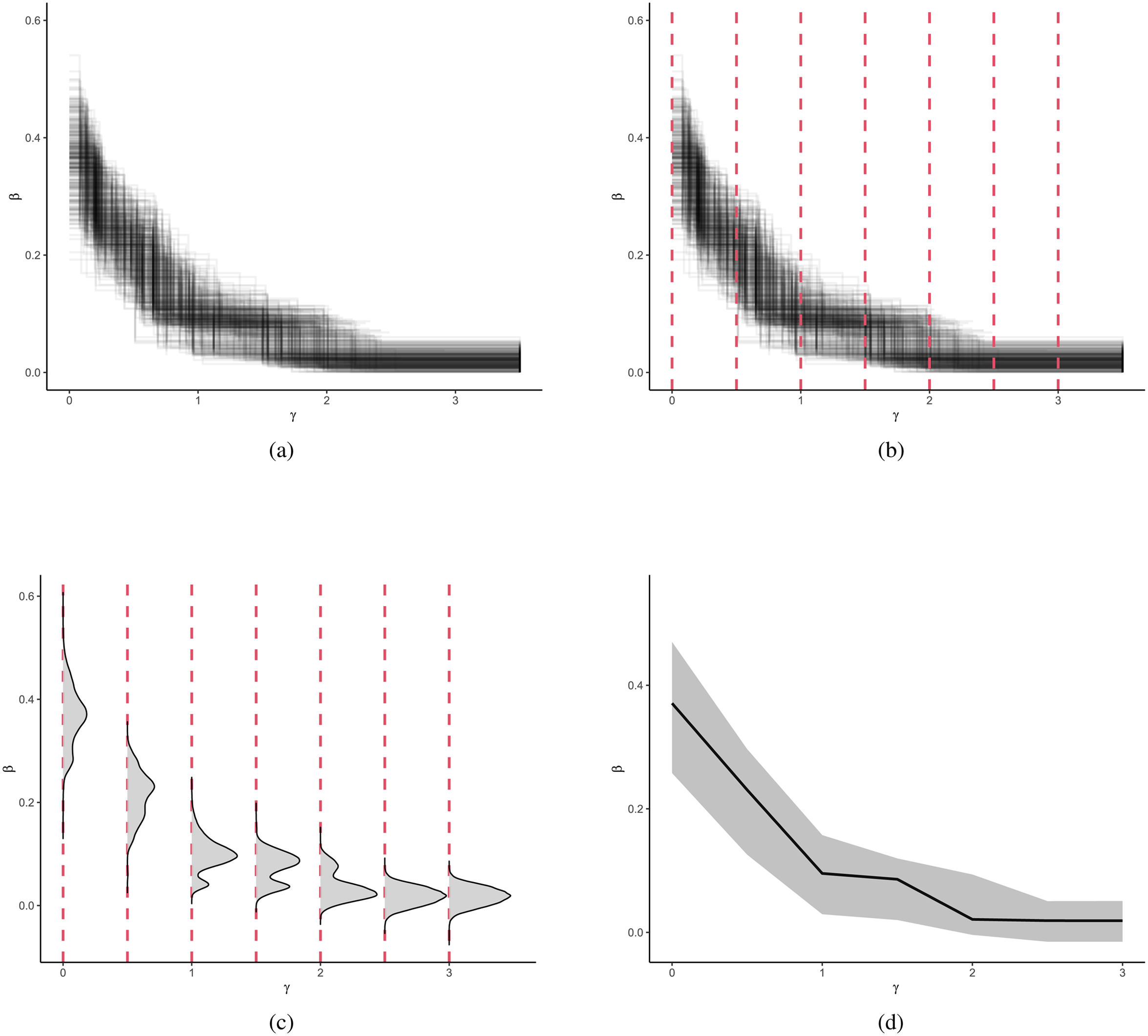
The estimate of the posterior decay is explained here in four plots: (a) Result of the Bayesian Model Averaging: posterior draws of (step-wise) $\beta$ generated by repeating step 1. and 2; (b) Estimating the posterior trend (first step): defining a dense grid of evenly spaced $\gamma$ ’s (vertical dashed red lines); (c) Estimating the posterior trend (second step): for each $\gamma$ the corresponding interval effect in each posterior step-wise draw is selected. The resulting density characterizes the posterior density at the specific $\gamma$ and (d) Posterior trend of $\beta$ : for each $\gamma$ and given the corresponding estimated posterior density (estimated in (c)), the posterior mode (solid black line) as well as the highest posterior density interval (shaded area) are estimated.

Computational details of the BMA

The most expensive step before estimating the posterior decay with the BMA is the estimation of all the $Q$ step-wise models in the bag. This subsection focuses on computational complexity of step-wise models compared to parametric decay models (e.g., exponential decay). We describe two stages where such models show differences in terms of their computational complexity: (1) the computation of endogenous statistics and (2) the estimation stage.

Calculation of endogenous statistics: A comparison on the number of operations performed in a single model

The computation of endogenous statistics is a time-consuming stage as it must be carried out across all the observed time points ( $M$ ) and for all the dyads that can occur over time. Without loss of generality we assume that at each time point all dyads are at risk of occurring, thus we consider the complete risk set as it is assumed in (1) where $D=|\mathcal{R}|=N\times (N-1)$ , with $N$ being the number of actors and $D$ the number of dyads in the risk set $\mathcal{R}$ . When a parametric weight decay is used (e.g., exponential decay), the computation of the endogenous statistics requires more operations than what is required in a step-wise model: the weight of past events has to be updated at each time point where an event is observed and according to the weight decay function. Such update requires the numerical evaluation of the decay function and this eventually increases the needed computational time.

The continuous update of the event weights is not required for the step-wise decay model where past events are assumed to have a unitary weight in each interval. Therefore, for a step-wise model the main steps for computing each endogenous statistic consist of: (i) at each time point defining the partitions of the event history according to the $K$ intervals describing the step-wise model, (ii) computing each endogenous statistic within such intervals. We optimize these two steps by minimizing the number of times that the algorithm has to compute the endogenous statistics according to each specific interval. Some time intervals might appear more than once along the event sequence. Therefore, we first find the time boundaries of the $K$ intervals across all the time points, then we consider the reduced set of intervals and calculate the endogenous statistics according to this reduced set. Finally, for each interval of the reduced set, the value of the endogenous statistics for all dyads is assigned to the correspondent interval in the original data-structure for the statistics, which is used in the estimation stage. This improvement makes the computation of the statistics faster since we avoid to compute the same statistic more than once. This optimization only works for endogenous statistics such as inertia, reciprocity, in-/out-degree, and other first-order endogenous statistics as well as for second- or higher-order endogenous statistics where the time order of the events doesn’t affect the value of the statistic.

The number of operations required in the computation of a single endogenous statistic can be quantified as follows:

In a step-wise decay model without our optimization, the number of operations is $(M-1)\times D\times K+(M-1)\times (K+1)$ , where $(M-1)\times D\times K$ consists of the number of times the statistic is computed, which is at each time point for each interval and for all dyads. We consider $M-1$ because at time $t_1$ all endogenous statistics assume value zero for all dyads. Furthermore, $(M-1)\times (K+1)$ is the total number of updates of the time boundaries characterizing the $K$ intervals throughout the event sequence. This step runs fast because it only requires simple subtractions between numbers;

In a step-wise decay model where our optimization is performed the number of operations is $\mathrm{\Psi }(\mathit{t},\mathit{\gamma })\times D+(M-1)\times (K+1)$ , where $\mathrm{\Psi }(\mathit{t},\mathit{\gamma })$ is the size of the reduced set of intervals; this is $\mathrm{\Psi }<(M-1)\times K$ and it depends both on the vector of observed time points $\mathit{t}=(t_1,\dots ,t_M)$ and on the vector of $K+1$ increasing widths $\mathit{\gamma }=({\gamma }_0,{\gamma }_1,\dots ,{\gamma }_K)$ that define the $K$ intervals over time. Furthermore, $(M-1)\times (K+1)$ again is the number of times we have to update the time boundaries before finding the reduced risk set;

In a parametric decay model (e.g., exponential, linear, or other decays) the number of operations is $(M-1)\times D+\frac{M\times (M-1)}{2}$ , where $(M-1)\times D$ is the number of times the statistic is computed and $\frac{M\times (M-1)}{2}$ is the number of total updates for the weights of the already-occurred dyads.

Let us compare the optimized step-wise decay with the parametric decay model. For this effort, we assume that: (i) $K$ is set to a low number around 3, 4 or 5 intervals; and (ii) the update of one single event weight requires as much computational time as the update of one time bound. Then, the number of updates in a parametric decay increases faster than in a step-wise decay. Indeed, the $(M-1)\times (K+1)$ operations for the computation of the time boundaries in the optimized step-wise model follow a linear function of the number of events ( $M$ ), whereas the $\frac{M\times (M-1)}{2}$ operations for the update of the weights in the parametric model follow a quadratic function of the number of events. Unfortunately, the optimized approach for the step-wise model cannot be performed on the transitivity closure introduced in Step-Wise Decay for Higher Order Endogenous Effects subsection, because the order of events in the triadic pattern matters. However, the optimization for the first-order statistics already saves much computational time, because in the estimation of more endogenous statistics the reduced set of intervals will be shared and calculated only once.

In Figure 9, we compare the running times for estimating inertia using four models: the optimized step-wise model with $K=\{3,4,5\}$ and the parametric decay model with exponential decay. Per each model, a set of intervals or half-life values were chosen, and their running times for computing inertia were repeatedly measured (each run of the algorithm was parallelized on 8 threads). Finally, every model has a total number of 1000 samples of running times. We performed such analysis on the empirical data used in Case Study: Investigating the Presence of Memory Decay in the Sequence of Demands sent Among Indian Socio-Political Actors section where the number of actors is $N=10$ , the number of dyads is $D=90$ and the number of events is $M=7567$ .

Figure 9.

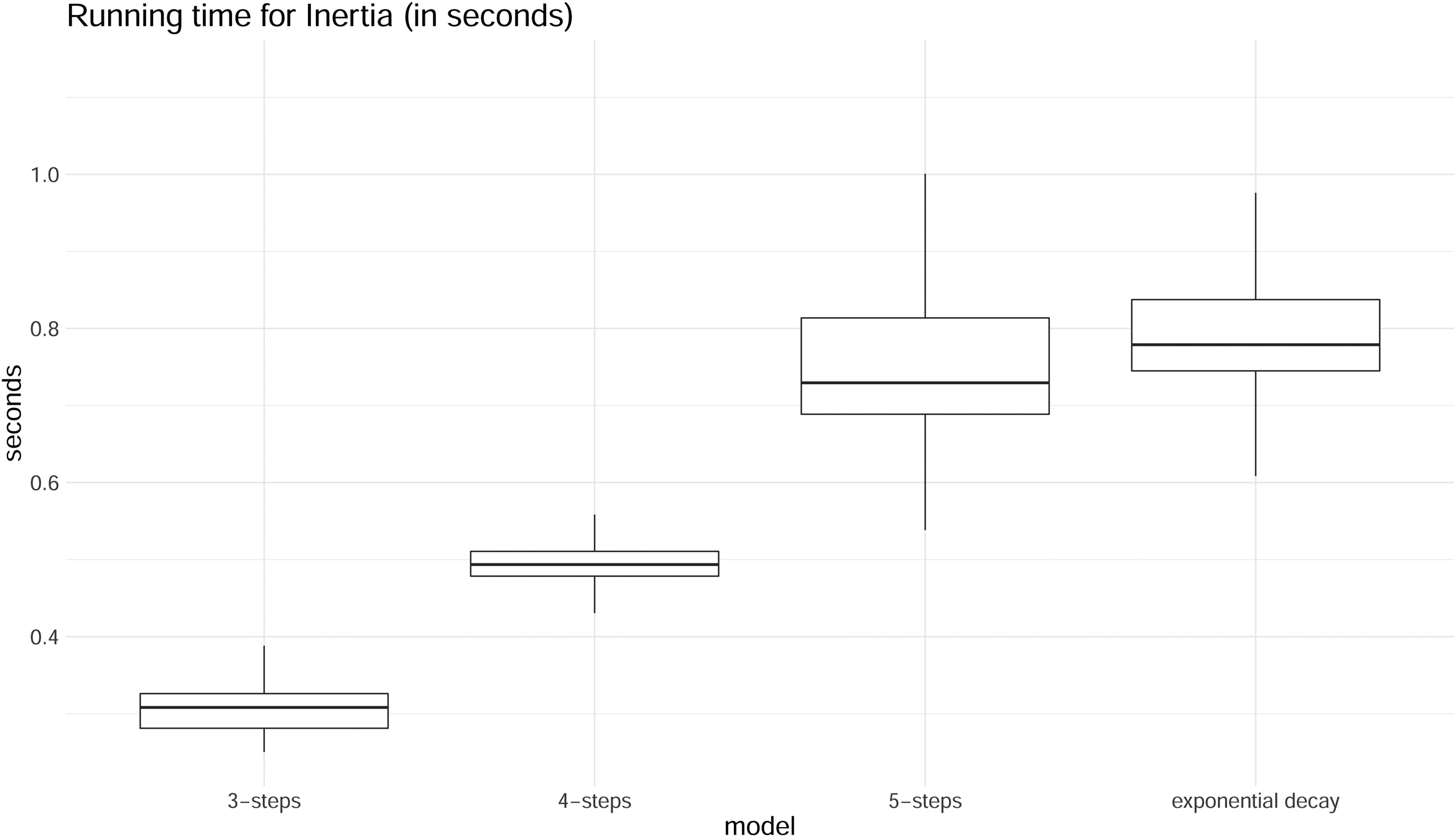
Distributions of running times for the endogenous statistic Inertia (in seconds). 3-steps, 4-steps and 5-steps models are compared to the parametric model with exponential decay. For each type of model, the running time was measured 1000 times.

Estimation stage: Comparison on the number of parameters to be estimated

Considering $U_{\text{exo}}$ exogenous statistics (including the intercept) and $U_{\text{endo}}$ endogenous statistics, in the estimation stage the total number of parameters to be estimated is

$U_{\text{exo}}+U_{\text{endo}}$ in REMs where endogenous statistics follow any parametric weight decay (e.g., exponential, linear, one-step decay);

$U_{\text{exo}}+(U_{\text{endo}}\times K)$ in step-wise REMs where $K$ is the number of intervals (steps) and all the endogenous statistics follow the same step-wise model.

Therefore, a step-wise model has always more parameters than a model with any parametric decay. However, this disadvantage at the estimation stage is not really an issue because it is not recommended to consider many intervals as the uncertainty around estimates increases when intervals become narrower and only a few events fall inside them.

Case study: Investigating the presence of memory decay in the sequence of demands sent among Indian socio-political actors

We have now introduced our modeling approach, starting from a purely step-wise decay model to a continuous decay model based on model averaging of a set of step-wise models. In this section, we illustrate the method by applying it to empirical data. First, we describe the empirical application and dataset. Next, we present analyses using different prespecified step-wise decay functions, followed by an application of the Bayesian model averaging estimated to obtain approximate smooth decay functions. Finally, we compare the semi-parametric model (that results from the Bayesian Model Averaging) with other relational event models where the memory decay is fixed either to a step-wise or exponential decay. In this comparison we focus on the predictive performance of the models as well as their resulting fit.

Relational events between socio-political actors

We retrieved data from the ICEWS (Integrated Crisis Early Warning System) (Boschee et al., 2015) repository, which is hosted in the Harvard Dataverse repository. ICEWS consists of relational events interactions between socio-political actors that were extracted from news articles. Information about the source actor, the target actor, and the event type is recorded along with geographical and temporal data that are available within the same news article. Event types are coded according to the CAMEO (Conflict and Mediation Event Observations) ontology. In this example analysis, we focus on the sequence of relational events within the country of India. Each event represents a request from an actor targeted to another actor. These requests range from humanitarian to military or economic in nature and in this analysis this distinction is not made.

The event sequence includes M = 7567 dyadic events between June 2012 and April 2020 among the ten most active actor types: citizens, government, police, member of the Judiciary, India, Indian National Congress Party, Bharatiya Janata Party, ministry, education sector, and “other authorities.” Since the time variable is recorded at a daily level, we consider events that occurred on the same day as evenly spaced throughout that day.

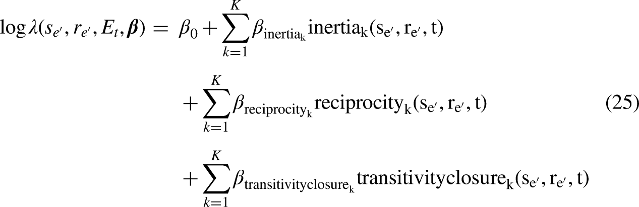
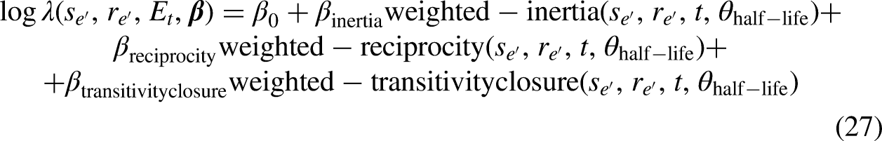
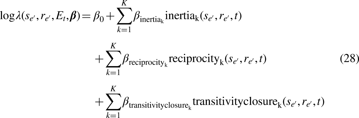
The network dynamics of interest are inertia, reciprocity, and transitivity closure. Given a generic step-wise model with $K$ steps, the log-rate at any time $t\in [t_1,t_M]$ and for any request $e^{\prime }$ is:

$$\begin{array}{rl}\log \lambda (s_{e^{\prime }},r_{e^{\prime }},E_t,\mathit{\beta })=& {\beta }_0+{\displaystyle \sum _{k=1}^K{\beta }_{{\text{inertia}}_k}{\text{inertia}}_k(s_{e^{\prime }},r_{e^{\prime }},t)}\\ & +{\displaystyle \sum _{k=1}^K{\beta }_{{\text{reciprocity}}_k}{\text{reciprocity}}_k(s_{e^{\prime }},r_{e^{\prime }},t)}\\ & +{\displaystyle \sum _{k=1}^K{\beta }_{{\text{transitivity closure}}_k}{\text{transitivity closure}}_k(s_{e^{\prime }},r_{e^{\prime }},t)}\end{array}$$

(25)

where ${\beta }_0$ represents the logarithm of the baseline rate of requests and the remaining effects describe the estimated step-wise trends for the three network statistics. Inertia quantifies the persistence of the sender in targeting its requests to the same receiver, for instance because the receiver is an actor with some socio-political relevance like a legal figure or authority. Reciprocity describes the level of reciprocation of the sender towards the receiver based on the past volume of interactions that the receiver addressed to the sender. Transitivity closure quantifies the level of information mediation by means of the volume of triads that can be potentially closed by the occurrence of event $e^{\prime }$ . We assume that at every point in time, every possible dyad is at risk of occurring, hence the risk set consists of $|\mathcal{R}|=N\times (N-1)=90$ dyads.

Predefined step-wise decay models

As the maximum time ( ${\gamma }_K$ ) that past events may affect current relational events we consider 180 days (roughly half an year). Furthermore, we consider three different predefined step-wise memory decay functions by dividing the past in $K=4$ intervals with either increasing widths, equal widths, or decreasing widths (as described in Generating a Bag of Step-Wise Relational Event Models subsection).

Figure 10 shows the estimated step-wise decay functions for inertia, reciprocity, and transitivity given the three different interval configurations.

Figure 10.

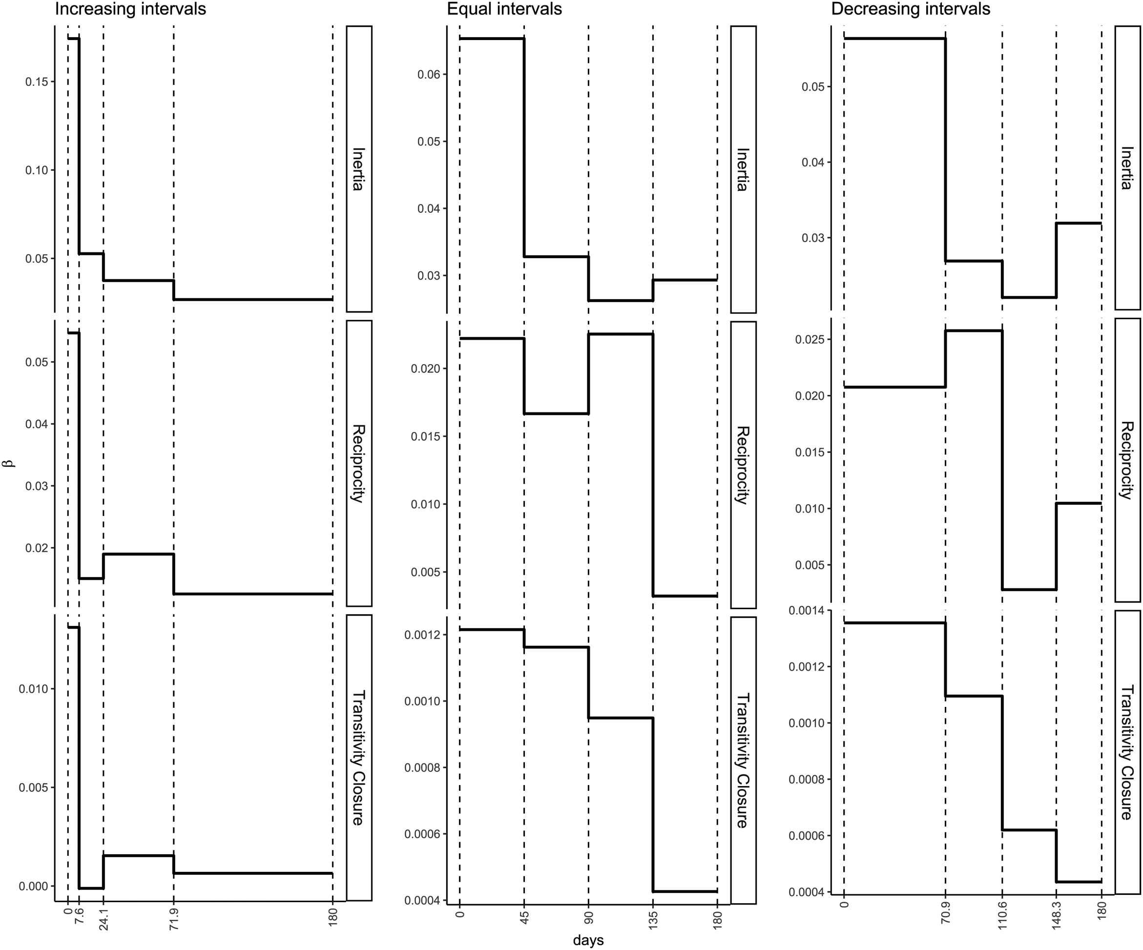
MLE estimates of $\hat{\beta }=\{{\hat{\beta }}_{{\text{inertia}}_1},\dots ,{\hat{\beta }}_{{\text{inertia}}_4},{\hat{\beta }}_{{\text{reciprocity}}_1},\dots ,{\hat{\beta }}_{{\text{reciprocity}}_4},{\hat{\beta }}_{{\text{transitivity}}_1},\dots ,{\hat{\beta }}_{{\text{transitivity}}_4}\}$ according to three different step-wise models (with $K=4$ ) that are randomly chosen from the bag of the estimated models and each following one of the three interval types (by column: increasing, equal and decreasing intervals). The bold black line represents the step-wise function for each endogenous effect in the model and the vertical dashed lines indicate the time bounds characterizing the intervals.

As is to be expected, the three models result in different estimated (discretized) shapes of memory decay. For instance, for Transitivity Closure we see that decreasing intervals and increasing intervals produce contrasting decays where the decays not only follow different shapes, but the magnitudes of the effect are different as well. The magnitudes of the effects are similar for the “equal” and “decreasing” intervals, whereas for “increasing” interval widths the magnitudes are quite different from the models with “equal” and “decreasing” widths.

In sum, step-wise models with predefined interval configurations provide us with a very rough idea of how fast memory decays in a given relational event network. However, predefined step-wise memory decay models provide only limited insight into the full shape of memory decay along transpired time, or, for example, whether an (approximated) exponential decay is more likely than a (approximated) smooth one-step decrease. To learn this from an observed relational event network, we need the proposed weighting system for a bag of step-wise models together with a Bayesian model averaging approach. We consider this next.

Approximately smooth memory decay models

For our bag of step-wise models, three sets of 501 intervals were generated for $K=\{3,4,5\}$ steps (250 intervals with increasing size, 250 intervals with decreasing size, 1 with equal size). Thus in total, 1503 step-wise models were considered. We chose to use around 500 models per $K$ since we noticed that the overall number of random intervals (1503) already provides stable final results. The estimation of the whole bag of models required about 6.5 hours: for each step-wise model the computation of the endogenous statistics as well as the estimation of parameters was parallelized on 8 threads ¹ .

Figure 11 shows the posterior trends resulting from two Bayesian Model Averaging approaches: one with BIC weights (left panels) and one with WAIC weights (right panels). Because most of the decay occurs in the first twenty days, only this period is plotted in the figure. The intercept ${\beta }_0$ is the only parameter without a decay by definition and the posterior point estimate of the baseline event rate is $\exp \{{\hat{\beta }}_0\}\approx 0.0129$ (similar for both BIC and WAIC weights; upper panels).

Figure 11.

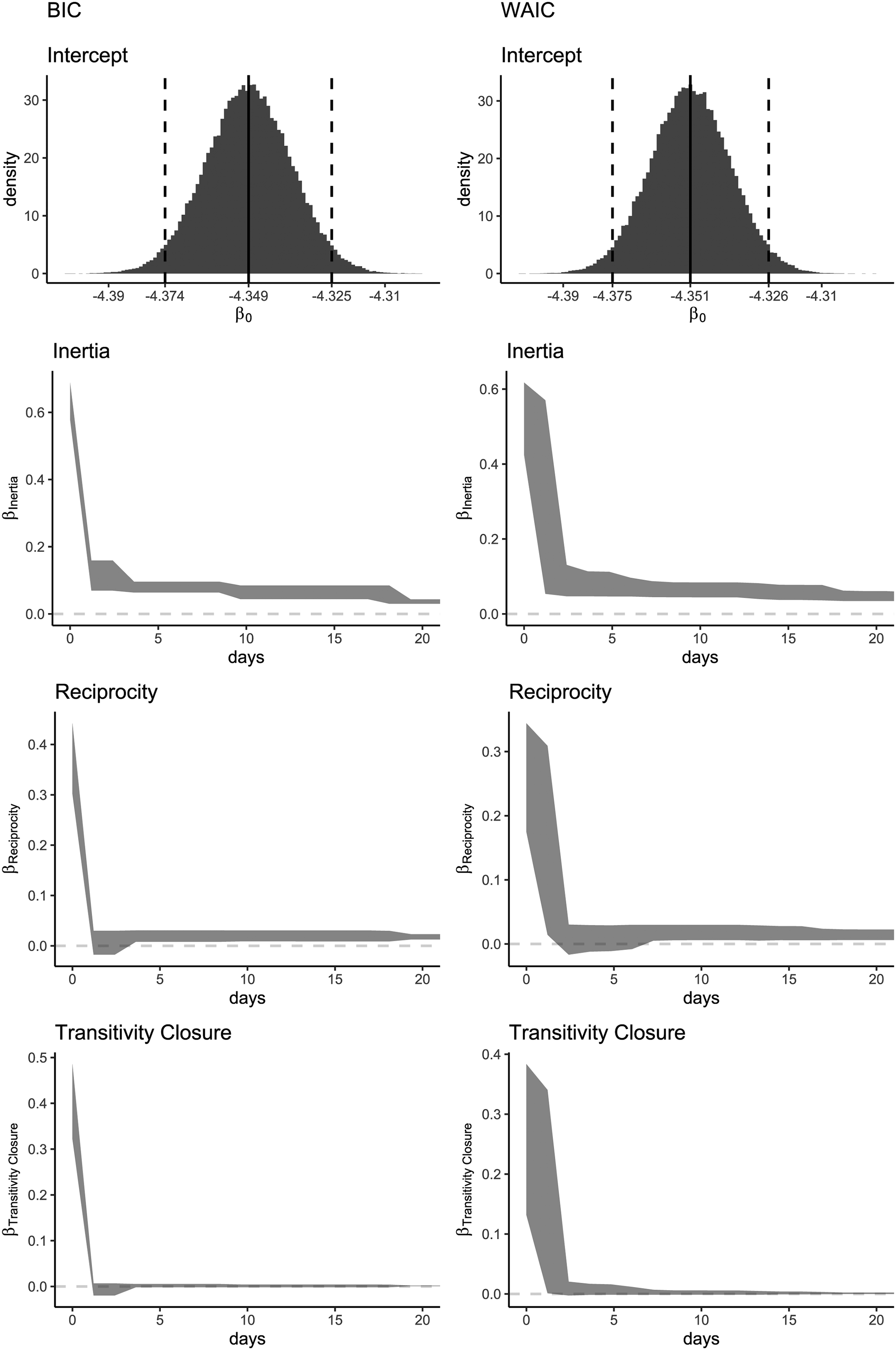
Posterior estimates resulting from the BMA with BIC (left) and WAIC (right) weights, from the top to the bottom: posterior distribution for the intercept ( ${\beta }_0$ ), posterior trends for inertia, reciprocity and transitivity closure. The gray area (dashed lines for the intercept) is generated by the highest posterior density intervals calculated until 20 days (maximum value plotted on the x-axis).

Since the network consists of nodes that represent collectives of individuals, it is important to interpret the estimated memory decay functions as referring to the memory of groups, rather than of individuals. Focusing on the results for the WAIC weights in Figure 11 (right panels), all the three trends show a clear approximately exponential memory decay. The drastic decrease near zero suggests that recent requests have a much higher impact on the event rate than less recent ones. Therefore, the trend observed for inertia indicates a tendency of actors to keep sending requests to the same recipient of their most recent requests. This reflects “short-lived inertia” (driven by the requests that happened in a fairly recent past) rather than “long-lived inertia” (where requests that have occurred over a much longer time span continue to be repeated).

For reciprocity, we see that memory drops a bit faster than for inertia and stabilizes around a low value that decreases further, indicating that actors reciprocate on requests received in the very recent past, but requests that were not responded to quickly are soon “forgotten” and are unlikely to be responded to. Norms of reciprocity are clearly not enduring and non-reciprocated requests disappear from social memory very quickly. Finally, transitivity is similarly driven by very recent interactions. Considering that dyadic requests only briefly trigger the tendency to respond, it makes sense that having common past communication partners also mainly matters if those joint interactions date back to only recent history rather than to a period somewhat longer ago.

Together, the results paint a picture of a “delusion of the day” kind of politics. Interactions between these institutional actors appears to be driven by current events in the country, where response to actuality appears more predictive of future interactions than long-term governed interaction. While this may be typical of governmental interactions, the effect may be strengthened by the fact that the data come from news paper articles. News paper articles will generally only report publicly visible interaction (hence, journalists may miss interaction that occurs behind closed doors or interactions that are not made public) and will tend to focus mainly on what is of interest “today.” That said, it does make a lot of sense to find that governmental parties seem to base their interactions mainly (but not exclusively) on what is going on in the present and the very recent past, and focus less on what happened longer ago and may be less salient in the public’s eye.

The resulting trends obtained from the BIC weights approximately follow the same decays as the WAIC. However, we see that the BIC weights show an approximate step-wise trend because the BIC becomes increasingly large for that step-wise model that is the closest to the true (smooth) model (in terms of Kullback-Leibler distance (Grünwald and Ommen, 2017)). Thus, the weight of that step-wise model dominates the weights of all other step-wise models. This illustrates that the BIC is useful for finding the best fitting step-wise model, which, in this case, has increasing interval widths over the transpired time, forming roughly an exponential decay. On the other hand, the BIC is less useful for finding an approximate smooth decay trend. For this purpose we recommend the WAIC.

Assessing the predictive performance: A comparison with parametric memory decays

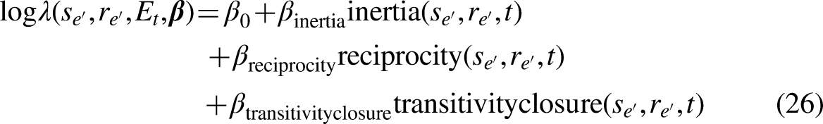
The results show that memory decays approximately exponentially in this dataset. Next, we compare the performance of the fitted semi-parametric model with other relational event models that either do not contemplate a memory decay (REM without memory) or fix it to some predefined parametric trend (step-wise or exponential):

REM without memory: this is a basic relational event model where endogenous statistics such as inertia, reciprocity, and transitivity closure are embedded in the linear predictor as a function of the total volume of past events without any memory decay. For the REM model without memory, the log-rate at any time $t\in [t_1,t_M]$ and for any request $e^{\prime }$ in the risk set $\mathcal{R}$ is:

$$\begin{array}{rl}\log \lambda (s_{e^{\prime }},r_{e^{\prime }},E_t,\mathit{\beta })& ={\beta }_0+{\beta }_{\text{inertia}}\text{inertia}({\mathit{s}}_{{\mathit{e}}^{\prime }},{\mathit{r}}_{{\mathit{e}}^{\prime }}\mathit{,}\mathit{t}\mathit{)}\\ & +{\beta }_{\text{reciprocity}}\text{reciprocity}({\mathit{s}}_{{\mathit{e}}^{\prime }}\mathit{,}{\mathit{r}}_{{\mathit{e}}^{\prime }}\mathit{,}\mathit{t}\mathit{)}\\ & +{\beta }_{\text{transitivity closure}}\text{transitivity closure}({\mathit{s}}_{{\mathit{e}}^{\prime }}\mathit{,}{\mathit{r}}_{{\mathit{e}}^{\prime }}\mathit{,}\mathit{t}\mathit{)}\end{array}$$

(26)

REM with exponential decay: We specify three models with endogenous statistics such that events follow an exponential weight decay. The weight decay at $t_m$ for any event occurred at $t_{e^{\prime }}<t_m$ is $\frac{\ln (2)}{{\theta }_{\text{half-life}}}\exp \{-(t_m-t_{e^{\prime }})\frac{\ln (2)}{{\theta }_{\text{half-life}}}\}$ (Brandes, Lerner, and Snijders, 2009), where ${\theta }_{\text{half-life}}$ is fixed, respectively, to 7 days, 30 days, and 90 days. For these models, the log-rate at any time $t\in [t_1,t_M]$ and for any request $e^{\prime }$ in the risk set $\mathcal{R}$ is:

$$\begin{array}{c}\log \lambda (s_{e^{\prime }},r_{e^{\prime }},E_t,\mathit{\beta })={\beta }_0+{\beta }_{\text{inertia}}\text{weighted-inertia}({\mathit{s}}_{{\mathit{e}}^{\prime }}\mathit{,}{\mathit{r}}_{{\mathit{e}}^{\prime }}\mathit{,}\mathit{t}\mathit{,}{\theta }_{\mathit{\text{half-life}}}\mathit{)}\mathit{+}\\ {\beta }_{\text{reciprocity}}\text{weighted-reciprocity}({\mathit{s}}_{{\mathit{e}}^{\prime }}\mathit{,}{\mathit{r}}_{{\mathit{e}}^{\prime }}\mathit{,}\mathit{t}\mathit{,}{\theta }_{\mathit{\text{half-life}}}\mathit{)}\mathit{+}\\ +{\beta }_{\text{transitivity closure}}\text{weighted-transitivity closure}({\mathit{s}}_{{\mathit{e}}^{\prime }}\mathit{,}{\mathit{r}}_{{\mathit{e}}^{\prime }}\mathit{,}\mathit{t}\mathit{,}{\theta }_{\mathit{\text{half-life}}}\mathit{)}\end{array}$$

(27)

These models are named Exp 7, Exp 30 and Exp 90 in Appendix A.4. The idea is similar to the approach of Brandenberger (2018) who also considers exponential decay models and uses different predefined values for the half-life parameter.

REM with step-wise decay: We specify three step-wise models with the following widths:

${\gamma }_{\text{days}}=\{0,90,180\}$ (two intervals with equal size);

${\gamma }_{\text{days}}=\{0,7,30,90,180\}$ (four intervals with increasing size);

${\gamma }_{\text{days}}=\{0,1.32,14,46.2,180\}$ (four intervals, using the widths of the model with the best WAIC found with the semi-parametric approach).

The step-wise models above are named respectively StepEqual, StepIncr and bestWAIC in Appendix A.4. The three models have ${\gamma }_{\text{max}}=180\text{days}$ . The log-rate at any time $t\in [t_1,t_M]$ and for any request $e^{\prime }$ in the risk set $\mathcal{R}$ is:

$$\begin{array}{rl}\log \lambda ({\mathit{s}}_{{\mathit{e}}^{\prime }}\mathit{,}{\mathit{r}}_{{\mathit{e}}^{\prime }}\mathit{,}{\mathit{E}}_{\mathit{t}}\mathit{,}\mathit{\beta }\mathit{)}=& {\beta }_0+{\displaystyle \sum _{k=1}^K{\beta }_{{\text{inertia}}_k}{\text{inertia}}_k({\mathit{s}}_{{\mathit{e}}^{\prime }}\mathit{,}{\mathit{r}}_{{\mathit{e}}^{\prime }}\mathit{,}\mathit{t}\mathit{)}}\\ & +{\displaystyle \sum _{k=1}^K{\beta }_{{\text{reciprocity}}_k}{\text{reciprocity}}_k({\mathit{s}}_{{\mathit{e}}^{\prime }}\mathit{,}{\mathit{r}}_{{\mathit{e}}^{\prime }}\mathit{,}\mathit{t}\mathit{)}}\\ & +{\displaystyle \sum _{k=1}^K{\beta }_{{\text{transitivity closure}}_k}{\text{transitivity closure}}_k({\mathit{s}}_{{\mathit{e}}^{\prime }}\mathit{,}{\mathit{r}}_{{\mathit{e}}^{\prime }}\mathit{,}\mathit{t}\mathit{)}}\end{array}$$

(28)

where $K$ is the number of intervals in the model. Endogenous statistics in step-wise models are calculated as explained in A Step-Wise Memory Decay Model section.

In Appendix A.4, we include a table with the maximum likelihood estimates and standard errors for each model.

In Figures 12 and 13, we examine two plots that assess the predictive performance of the models.

Figure 12.

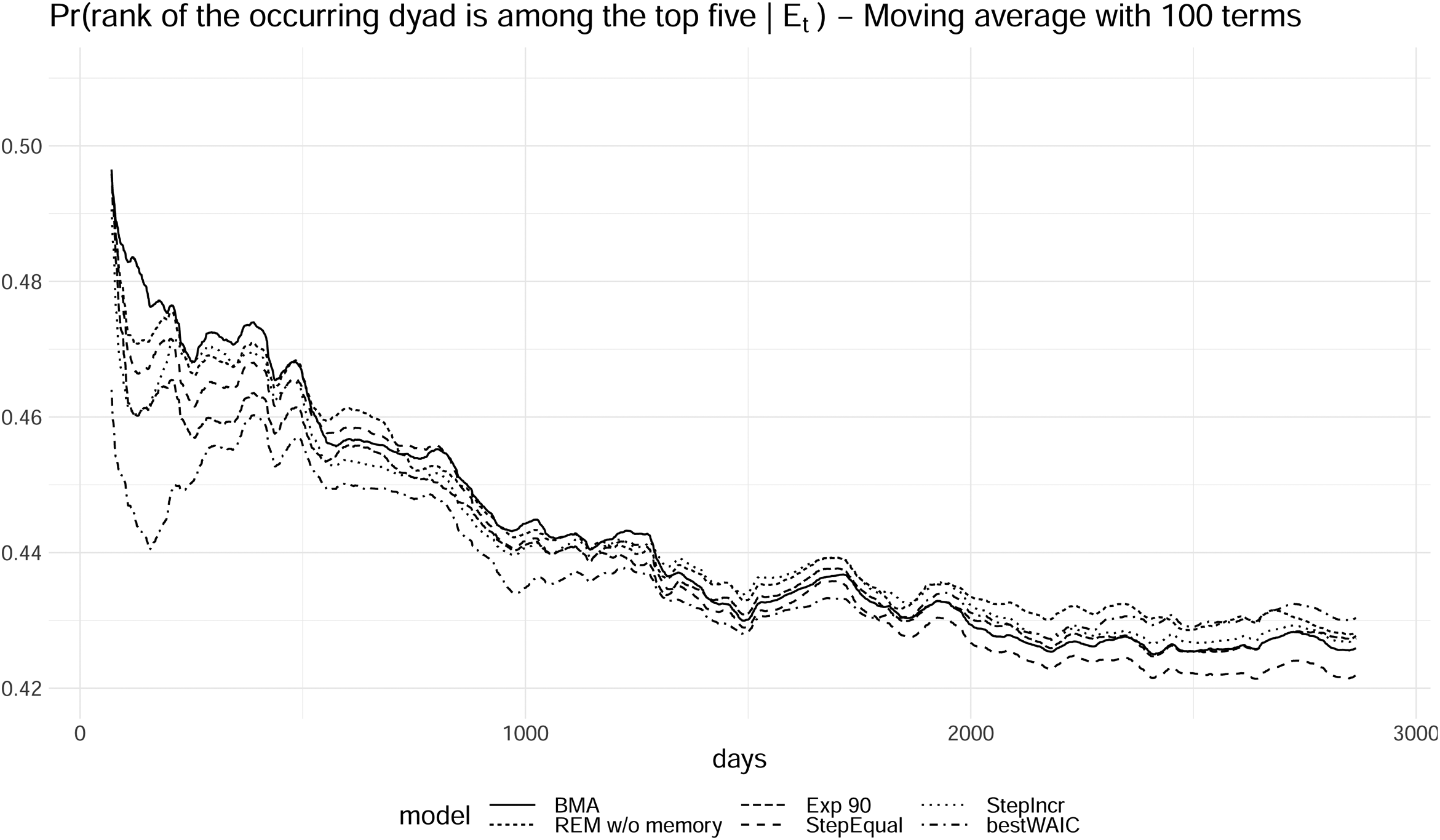
Probability of observing the rank of the occurring dyads being among the first five most likely dyads (moving average with 100 terms, Exp 7 and Exp 30 performed worse than the rest of the models and were removed from the plot).

Figure 13.

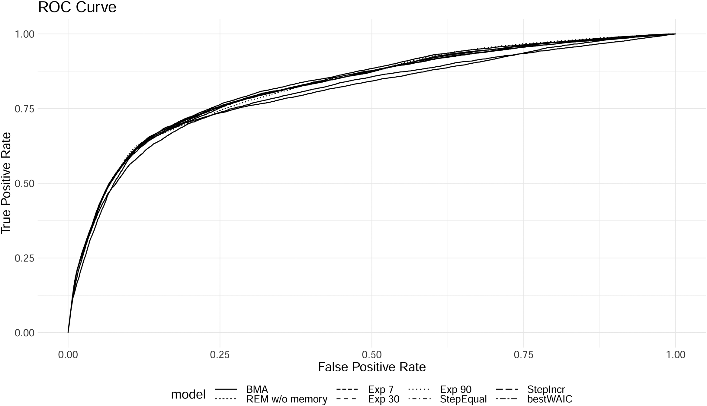
ROC curve of each model in the comparison.

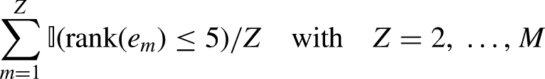
Figure 12 displays the probability of the observed dyads having rank less or equal than five, calculated as

$$\sum _{m=1}^Z\mathbb{I}(\text{rank}({\mathit{e}}_{\mathit{m}}\mathit{)}\le 5)/\mathit{Z}\mathit{\text{with}}\mathit{Z}\mathit{=}2,\dots ,\mathit{M}$$

where $\text{rank}(e_m)$ returns the rank of the predicted probability for event $e_m$ and $M=7567$ is the number of events in the sequence. Thus, at each time point, given the sequence of already occurred events (including the occurring event at $t_m$ ), the count of predicted ranks being less or equal than five (out of the 90 dyads that were at risk at each time point) is divided by the number of events in the partial event sequence. We calculate this probability for all models under comparison. We consider a moving average with 100 events to better visualize the overall predictive trends. We excluded models Exp 7 and Exp 30 from the figure because they performed clearly worse than the rest of the models (this keeps the figure more readable).

The plotted trends show how well the models perform over time. The solid line represents the performance of the BMA model resulting from the semi-parametric approach introduced in this paper. In comparison to the other decay models, its performance maintains a level that is, on average, higher than most of the models in the comparison. This illustrates that a model where the shape of the decay is learned from the data on average results in better predictions and better model fit than competing models where the decay is prespecified based on rough heuristic arguments. Finally it is interesting to observe that the REM without memory also performs quite competitively.

We note that the aim of our approach is not to generate a model that necessarily outperforms other models in predictive accuracy. Although the model is expected to generally do equally well or better than most competing models, an important aspect of the approach is that it allows a researcher to get a good idea of how long past events maintain their influence. This allows a researcher to then specify better further inferential models (informed by the decay shape that is found from the semi-parametric model). Perhaps more importantly, empirical results of exactly how the past keeps influencing the present and the future are essential for theory development. Considering the dearth of time-sensitive social theory, approaches that can uncover the empirical pattern of time can be highly informative for theorists to develop truly time-sensitive social theories upon. Of course, this requires the application of the model to a wider set of data than just our illustrative data set.

We plot the ROC curves in Figure 13; again we see that the BMA model on average performs best. Here, the REM without memory performs relatively poorly. The no-memory REM under-predicts actually occurring events and can only achieve high accuracy by predicting a relatively large number of events that actually do not occur. The memory-based models have a better overall trade-off between incorrectly and correctly predicted events, even considering the simplicity (the models are fully based on only inertia, reciprocity, transitivity closure, and an intercept) of the model for such complex interaction patterns among governmental actors in India.

Discussion

In this paper, we presented different methods for learning how past interactions between social actors affect future interactions in the network. We first considered a $K$ -step-wise model that approximated memory decay with a discrete step-wise trend. This model can be estimated using existing software functions for relational event analysis. The proposed Bayesian model averaged memory decay estimator will be made available in a new R package.

The next key contribution is a novel Bayesian model averaging approach to estimating memory decay in a relational modeling framework where events are assumed to continuously change in importance as the time since the event increases. The promising aspect of this semi-parametric approach lies in its ability to learn the shape of the memory decay without making any parametric assumption about it. Furthermore, by building on the step-wise model, the proposed method is computationally feasible. We considered two weighting systems for Bayesian model averaging of a bag of step-wise models: the BIC and the WAIC. As was illustrated, the BIC is useful for finding the one best fitting step-wise model for a given empirical relational event history. The BIC, however, is not suitable for finding an approximate smooth trend of the memory decay, as all weight is placed on the single step-wise model that is closest to the true smooth decay model. This issue does not occur for the WAIC as the Bayesian model average of many step-wise models results in a smooth trend.

The semi-parametric approach on average provided better predictive performance than other approaches where the weight decay was set using predefined parameters. This illustrates the usefulness of relaxing the assumption of predefined decay functions when making predictions and doing inferences. Moreover, the semi-parametric approach can uncover exactly how and for how long past events matter and can show if this is perhaps different between reciprocity and transitivity (or other statistics). A researcher can use the semi-parametric approach to first run several relatively simple models that can inform the researcher about the memory decay shapes that are present in the data at hand. Following that, the researcher can then specify further, more complex, models that utilize some predefined memory structure that is based on the shape found by the semi-parametric approach. This allows a researcher to run quite complex relational event models, without the computational burden of repeating the memory decay model several times for each new model that is specified, while, at the same time, taking into account the empirically extracted memory decay function for the dataset at hand.

In addition, researchers can use the methodology to uncover empirical trends of how past events matter as time passes by. Once this has been applied to enough datasets, these findings can inform solid theory development on how the past matters for the future. There is barely any social theory that is able to systematically explain and predict how present social interaction affect future social interactions and for how long exactly, whether the effects are linear or non-linear (and, in which case: following which shape?), and which conditions have an effect on that. Although social scientists acknowledge that time and timing matters for social reality (e.g., Leenders, Contractor, and DeChurch et al. (2016); Ancona et al. (2001); Monge (1990); Mitchell and James (2001); Kozlowski et al. (2016)), the empirical means to uncover actual memory shapes or the empirical means to test potential theoretical expectations about the course of time has lacked. We believe that our approach has the ability to support these efforts.

In this paper, we assume that all events are random, in the sense of having some probability of occurrence at any time. Some events, however, are not random and follow a fixed deterministic pattern. Marcum and Butts (2015) refer to these events as “clock events”. Examples include standardized lunch times (“every day we eat together in the cafeteria between 1200h and 1230h”), fixed office hours, the end of the workday at 1700h, et cetera. These deterministic events can affect interaction rates directly, but can also affect memory decay. For example, consider a workplace where work ends strictly at 1700h. If it happens to be the norm to follow up on a request from a colleague within half an hour (and older requests “drop from the radar”), requests that come in at 1645h should be handled within fifteen minutes and may be forgotten as the clock turns 1700h. In this case, the deterministic end-of-workday event directly affects the memory decay. In situations where clock events occur, it would be interesting to incorporate them into the modeling approach. At the very least, the researcher should be aware of them, so as to not have the memory shapes be affected by the clock events without the researcher realizing it.

The empirical example presented in this paper involves a relatively small network. It is important to note however that the methodology can be used for larger networks as well, even though the computation can be expensive in that case. We leave computational optimization of the approach for larger networks for future work.

Another important direction for future research would be to apply the method to different event types or sentiments. For instance, one expects negative events (e.g., a country threatening another country, a pupil insulting a peer, a teacher rebuking a student) to have a memory decay that is slower and more persistent than for positive events (e.g., a teacher praising a student, a country cooperating with another country) (Brass and Labianca (1999); Labianca and Brass (2006)). This difference may apply as well to other event types from which possible different memory shapes might emerge. For example, it might be that email interaction is more fleeting than face-to-face interaction. This is especially relevant in the understanding of projects where some project members may be co-located and have ample face-to-face interaction, while other members of the project team may reside in different locations which makes technology-enabled communication with them more pertinent. The team leader may give a similar message to a co-located project member (using face-to-face interaction) as to a physically-distant project member (sending an email), where the two communication media may have differential memory effects. Having a modeling approach like the semi-parametric model from this paper allows researchers to study conditions that affect memory decay patterns differently.

Furthermore, in the case of more dynamic situations, e.g., when the network switches between different states or regimes, memory decay may also change accordingly. For example, in emergency situations, recently past events may play an even larger role on interaction dynamics than long past events compared to the period of time before the emergency happened. Consequently, we would want to learn the change of the shape (and length) of memory decay across different states in dynamic environments.

In our approach, we do not prespecify the shape of the memory decay. However, with the choice for BIC or WAIC and with the choice for increasing/decreasing/equal intervals, some shapes are more likely to be found than others. We have illustrated how a researcher can compare these various choices against each other and pick that specification that fits the data best (according to predictive fit or some other criterion). However, a substantively very meaningful next step would be to examine when it is more plausible for memory decay to follow a step-wise or a continuous shape. It is worth it to systematically examine which social mechanisms are likely to lead to step-wise temporal effects and which mechanisms are not. This would both assist further model building and the further development of time-sensitive social theory.

We expect that the acquired ability of both estimating social memory decay processes and testing for the various conditions that might shape them can be a crucial step towards a more accurate understanding of network dynamics developing at a local as well as at a global level.