Sage Journals: Discover world-class research

Abstract

It is widely recognized that segregation processes are often the result of complex nonlinear dynamics. Empirical analyses of complex dynamics are however rare, because there is a lack of appropriate empirical modeling techniques that are capable of capturing complex patterns and nonlinearities. At the same time, we know that many social phenomena display nonlinearities. In this article, we introduce a new modeling tool in order to partly fill this void in the literature. Using data of all secondary schools in Stockholm county during the years 1990 to 2002, we demonstrate how the methodology can be applied to identify complex dynamic patterns like tipping points and multiple phase transitions with respect to segregation. We establish critical thresholds in schools’ ethnic compositions, in general, and in relation to various factors such as school quality and parents’ income, at which the schools are likely to tip and become increasingly segregated.

Keywords

dynamical systems tipping points nonlinearities social systems segregation school segregation

Introduction

Thomas Schelling’s work on segregation dynamics (1969, 1971) has been enormously influential. His analyses brought to the fore how highly segregated outcomes can emerge even when all individuals involved would prefer nonsegregated outcomes. While Schelling’s model has mainly been used for analyzing neighborhood segregation, the core mechanisms are general and they are at work in other types of segregation processes as well, such as those leading to segregated schools (Caetano and Maheshri 2013; Card, Mas, and Rothstein 2008; Burgess et al. 2005; Noreisch 2007; Saporito and Lareau 1999). When individuals with certain sociodemographic characteristics leave a school, they change the sociodemographic composition of the school, and this may prompt others to leave, which again changes the sociodemographic composition of the school, triggering further reactions. In this way, even small initial events can set in motion dynamic processes with considerable long-term effects.

Schelling’s analyses also highlighted the importance of focusing on complex dynamics like “tipping points” in order to explain observed segregation processes.¹ A tipping point is a state of a system at which the dynamics change in qualitatively important ways. For example, the tipping point may refer to the percentage of students with foreign-born parents at which students with native-born parents start to leave the school at an increasing rate. A given change in the proportion of students with foreign-born parents may have a huge effect on the collective outcome if it occurs in the vicinity of a tipping point, while it may have little or no effect if it occurs elsewhere. Therefore, if we want to understand how segregation processes are likely to unfold, we need to identify points at which systems are likely to tip.

Over the years, Schelling’s ideas have been used and elaborated in various ways but mostly in purely theoretical models (Pancs and Vriend 2007; Zhang 2009). Until recently, many researchers were skeptical about the possibility of deriving tipping points empirically, because tipping points were assumed to be too variable historically, demographically, and socially (Goering 1978). More lately, several studies have tried to identify tipping points empirically however. One important example is Card et al.’s analyses of neighborhood tipping (2008). They used regression discontinuity methods and U.S. census tract data from 1970 through 2000 to test hypotheses about ethnic-based tipping behavior. They found that the behavior of the white population exhibited tipping-like behavior in most cities, with a distribution of tipping points ranging from a 5 percent to a 20 percent minority share.

The analyses of Card et al. have been criticized by Caetano and Maheshri (2013) for assuming that all neighborhoods within a city have the same fixed tipping point. Using a combination of statistical and agent-based simulation analyses, their own school segregation analyses suggest considerable between-school variations (Caetano and Maheshri 2013). In fact, the conclusion that there is no single typical tipping point was already made by Quercia and Galster (2000) who reviewed theories and empirical literature concerning thresholds related to neighborhood change. Instead, Quercia and Galster (2000) found many different tipping points that varied according to a host of factors.

What is often overlooked in research with a focus on finding tipping points is that there may be other dynamics at work which possibly are also of importance for understanding the complexity of phenomena like segregation. Searching for single or typical tipping points may lead researchers to overlook for instance multistate effects, where the tipping behavior itself is changing in interaction with other factors and with the transforming state of the social system. We need therefore not only a way to identify single tipping points but rather a way to identify the best fitting pattern for a nonlinear social process selected from a range of possible complex patterns.

In this article, we introduce a new dynamical systems modeling technique for deriving empirically complex dynamics like tipping points, multistate effects, acceleration, and decelerating processes, to name a few. This method allows us to include several variables that may have complex nonlinear effects of their own and in mutual interaction.

We apply this methodology to analyze school segregation dynamics in Sweden. We derive a common model for all schools, but our approach allows for different dynamics, tipping points, and trajectories for different schools depending upon various attributes of the schools. School segregation is a rather well-studied phenomenon. Compared to other Nordic countries, Sweden has a high level of school segregation, which moreover has increased over time (Skolverket 2006; Utbildnings och kulturdepartementet 2006). Since the early 1990s Sweden has a free school choice system and according to many scholars, school choice has increased the segregation level of schools in Sweden (Andersson, Malmberg, and Östh 2012; Andersson, Östh, and Malmberg 2010; Bunar and Kallstenius 2005; Söderström and Uusitalo 2010; Trumberg 2011). Studies have shown that schools are often chosen based on their ethnic and socioeconomic composition (Burgess et al. 2005; Karsten et al. 2003; Noreisch 2007; Reay 2004), and several studies have suggested that self-segregation mechanisms may be important (Bunar 2010; DeSena 2006; Johansson and Hammarén 2010). The self-segregation mechanism is further reinforced by the fact that schools of lower performance tend to recruit students rather locally compared to high performing schools (Butler et al. 2007; Trumberg 2011). School choice therefore seems to reinforce the segregation of those schools that are already at risk of becoming segregated because they are located in segregated neighborhoods.²

Most studies of school segregation look at individual-level data although segregation is a property of supra-individual entities such as schools and neighborhoods. The reason for using individual-level data is to understand the micromechanisms generating the observed segregation patterns. But, looking only at the individual-level data means that we may not capture the systemic dynamics that social phenomena display on the aggregate level: nonlinearities, negative and/or positive feedbacks, and so on. Systemic dynamics are brought about and are supervenient upon micro-level processes, but they often are extremely difficult to derive from the micro-level behavior of individuals. It is therefore necessary to also study systemic dynamics on their own in order to fully understand the segregation dynamics. Here we present an approach to study such systemic dynamics using aggregate school data. In contrast to classic approaches to identifying tipping points that try to establish strict causality, that is, changes in demographic composition that lead to a causal response on the individual level (Caetano and Maheshri 2015), the dynamical systems approach presented in this article allows for mutual interactions, feedbacks, and reinforcements that do not necessarily follow a clear causal pattern. For clear causal interpretation, either experimental approaches or some sort of instrumental variables, which however are very difficult to find in practice (Bowden and Turkington 1990; Caetano and Maheshri 2015), would be necessary. The variables included in our analysis are known to be strong predictors from earlier research on school choice and school segregation (Andersson et al. 2012; Andersson et al. 2010; Bunar and Kallstenius 2005; Söderström and Uusitalo 2010; Trumberg 2011). However, our data are not experimental data and the variables at hand turned out not to be instrumental variables, as they affected both the predictor and the outcome variable. If appropriate instrumental variables could be found, they could be easily incorporated into the dynamical system approach used here, which would then facilitate causal interpretations of results. Generally, the strength of our methodological approach lies not so much in identifying clear causal effects, but rather complex interactive, coupled system dynamics that enhance our understanding of the system and its often nonlinear dynamics as whole and that allows for predictions on the social system level.

The rest of the article is organized as follows: In the next section, we provide a brief theoretical background to the approach adopted here. Thereafter, we introduce our modeling approach and we describe the data to which the method will be applied exemplarily. This is followed by a detailed presentation of the empirical results. We conclude by summarizing the main results and with a brief discussion of the methodological implications of our analyses.

Complex Dynamics, Tipping, and Segregation Dynamics

Dynamical system is a common mathematical approach in complexity sciences (Bossel 1994; de Vries 2013; Meadows 2008; Richardson 1991) and is receiving increasing attention in the social sciences. The aim of dynamical systems modeling is to go beyond conventional linear modeling when studying complex social processes (Andrey, Andreev, and Levandovskii 1997; Campbell and Mayer-Kress 1997; Hatt 2009; Zambelli and George 2012).

One prominent nonlinearity pattern in segregation dynamics is tipping behavior. Drawing upon ideas about phase transitions in physics, Morton Grodzins introduced the concept of the tipping point and thresholds into the social sciences in a study of the segregation of U.S. neighborhoods (1957, 1958). As the concept is used here, the tipping point is a macro-level property characterizing schools (or other social entities). It is a property that is definable only for a collectivity of individuals but not for any single member of the collectivity (Hedström 2005). Individuals’ actions bring about changes in the composition of schools, and their actions can be influenced by the properties of the schools, but it is the schools that tip and the tipping points refer to these collective entities.

The same applies to other complex patterns like multistate effects. We speak of multistate effects, if a social system has multiple states at which phase transitions can occur. Applied to the case of school segregation this means that schools’ tipping behavior may be far more complex than assumed in most of the previous literature. Tipping phenomena may not be the result of some critical ethnic school composition but rather the result of the interplay between ethnic school composition and other relevant factors, like the schools’ socioeconomic characteristics or the schools’ quality.

We now make the notion of a tipping or a phase transition more precise. In Schelling (1971) tipping behavior, a discontinuity between the current and future neighborhood composition, arises when the share of minorities m in a mixed neighborhood rises above a threshold that depicts a minority share m* that white neighborhood inhabitants are willing to tolerate. Even if the threshold is assumed to vary among the white residents, a random variable distributed across the white population with some distribution function f(), tipping behavior is likely to arise. A fraction of the white population will tolerate a certain minority share m* in their neighborhood, but if the minority share m rises above this threshold, this fraction of white inhabitants will leave the neighborhood, which will result in further increase of the minority share in that neighborhood, which in turn will affect another fraction of whites with a higher threshold m**, that is now surpassed as well—a cascade of white flight is initiated. The dynamic is illustrated in Figure 1.

Figure 1.

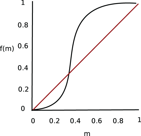
Tipping point model in Schelling (1971), cf. also Card, Mas, and Rothstein (2006), with f(m) depicting the distribution of white inhabitants with various minority share thresholds and m representing the minority share in a neighborhood. The 45-degree red line represents the capacity of the neighborhood, when f(m) = m.

Card et al. (2008) expanded Schelling’s model of tipping based on minority share, by including housing prices as an additional factor. And Caetano and Maheshri (2013, 2015) applied Schelling’s tipping model to school segregation, extending the model to other factors that may play a role in school choice, besides the minority share in a school. The minority share m of a school at t₀ is conceptualized as a function f() of the minority share m in that school and other school characteristics X_i at a previous point in time t₋₁. The change in m is a result of aggregate white and minority parental demand function, based on the school’s minority share and other characteristics. Following Schelling (1971), Caetano and Maheshri (2013, 2015) define a tipping point as a point on the curve that crosses the 45 degree line from below (see Figure 1).

More recently, Lamberson and Page (2012) suggested an updated conceptualization and formalization of tipping. Tipping points based on Schelling’s tipping model are all direct tips, they occur when a gradual change in a variable leads to a discontinuous jump in the value of this variable in the future (Lamberson and Page 2012). Lamberson and Page suggest a second type of tipping, contextual tips, which often explain the direct tipping. A contextual tip occurs when a gradual change in the value of one variable leads to a discontinuity in some other variable (Lamberson and Page 2012). Lamberson and Page moreover use mathematical formalism of dynamical systems to define tipping points as discontinuities in the relationship between present conditions and future states of the system:

“Let x_t, y_t and z_t be dynamic processes such that future states of x_t are determined by the current states of x_t, y_t and z_t which belong to Ω _x , Ω _y , and Ω _z respectively. We call the variable x _t the tipping variable and y_t the threshold variable and use z_t as a place holder for anything else that might affect the function value. (…). To capture the effect of present condition on the future, we introduce a function L_Δ(x_t, y_t, z_t) = x_t+_Δ, which gives the value of x_t exactly Δ steps after t (…). A point τ ∈ Ω_y is a tipping point for x_t, if there exists a path q: (−1, 1) → Ω_y with q(0) = τ such that L_Δ(x_t, q(s), z_t) is discontinuous as a function of s at s = 0 for some Δ > 0. (Lamberson and Page 2012:178-79)”

That is, small changes in y_t near the threshold point τ cause the future path of x_t to drift apart. In our conceptualization of tipping points, we largely follow the approach suggested by Lamberson and Page (2012). Let us assume that Y is the indicator we are interested in, the tipping variable in Lamberson and Page (2012) terms. We are interested in the rate of change in Y over a time interval, dt, as a function of itself and a threshold variable, X₁ and other relevant variables X₂, X₃, …, X_n.

Specifically, we focus on

\frac{d Y}{d t} = f (Y, X_{1}, X_{i}) .

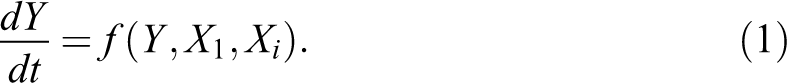
The rate of changes in Y thus is a function of the threshold variable X₁ and other variables X_i from a set of relevant factors.

We identify tipping points to be the points at which f(Y, X₁, X_i) changes sign from positive to negative, thus representing a discontinuity that shifts the system from one equilibrium (positive changes) to another (negative changes), in response to a change in the threshold variable, X₁. These points are identified by finding X_* such that

f (Y, X_{*}, X_{i}) = 0.

We call this equation defining X_* the threshold equation, identifying the critical X₁ values at which Y tips. Typically, X_* is a function of the other variables, including Y, and not a uniquely defined point.

The empirical approach adopted here implements this formalization. In our empirical application, example Y is the proportion of students of Swedish origin (S) in a school and X₁ is a variable measuring the degree of perceived foreignness (F) of the minorities represented in the school, while other relevant variables measure factors like school quality and socioeconomic characteristics of the students (see Data subsection for details). In the empirical application of our methodological approach, we therefore focus on:

\frac{d S}{d t} = f (S, F, X_{i}) .

This gives us the rate of change in the proportion of students of Swedish origin as a function of the perceived foreignness due to the school’s overall ethnic composition and other variables from a set of relevant factors. The tipping points in the threshold variable, F_* (tolerated maximum perceived foreignness of minorities in a school) are identified by setting f(S, F_*, X_i) = 0. F_* would be a function of S and X_i in our empirical case. Hence, the approach meets Caetano’s and Maheshri’s (2011, 2013, 2015) reasonable demand that models of tipping behavior must allow for the possibility that the aggregate units may differ from one another in respect to various attributes of relevance for the tipping points. For instance, schools may vary from one another in such a way that a unique and common tipping point is unlikely to be observed.

Data and Methods

Methods

As mentioned earlier, a narrow focus on tipping behavior only may lead to overlooking of other nonlinear dynamics in a social system. The method we introduce here does not only allow us to identify tipping in a rather straightforward way, it allows us also to capture various other complex patterns. More specifically, we are using a methodology called Bayesian dynamical systems modeling, outlined in Ranganathan et al. (2014).

Based on theoretical considerations and results from previous research, we specify the variables likely to be of relevance for explaining changes in the ethnic composition of schools. We then allow the data to do as much of the talking as possible in order not to let preconceived notions unduly influence the specification of the models and thereby also the results. We use panel data to model changes and we do this by estimating the parameters of ordinary differential equations.

Our basic approach is to fit ordinary differential equation models to available panel data. For each variable, we model changes in one variable between times t and t + 1 as a function of all included model variables at time t. In a model with only two variables X, Y, a dynamical system would be represented by a system of two differential equations:

\frac{d Y}{d t} = f_{1} (Y, X) .

\frac{d X}{d t} = f_{2} (Y, X) .

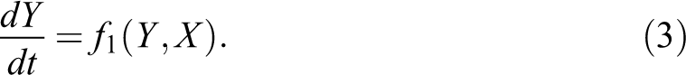
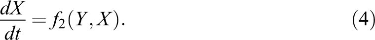
In order to model as many nonlinearities as possible, we take each f_i(.) to be polynomial of sufficiently high degree. Specifically, we define a set of polynomial terms that allow us, on the one hand, to model a number of different complex dynamics and, on the other hand, keeps the number of evaluated models sufficiently small. We note here that if prediction were the most important goal of modeling, various nonparametric approaches from the machine learning literature may be used to model the changes in Y and X (Bishop 2006; Li and Racine 2007). Since we want to understand the process also in terms of the mechanisms involved, we use polynomial terms which provide us some insight into how the changes take place. In a two-variable model, we therefore study models f(Y, X) of the form:

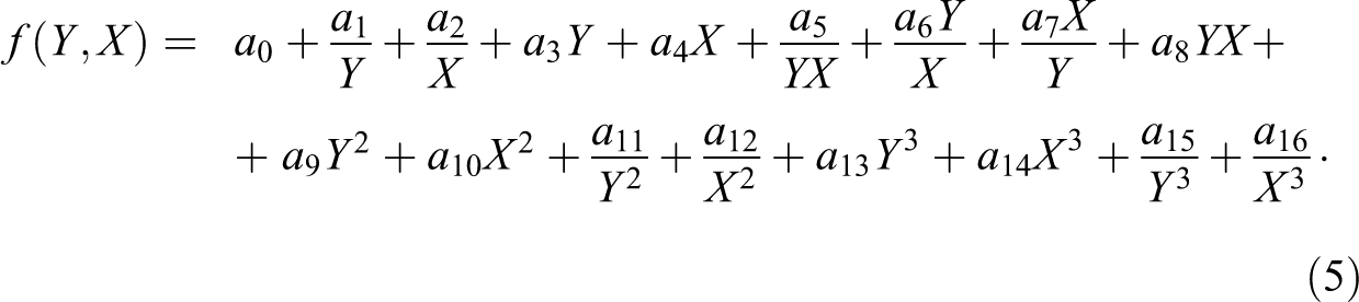
\begin{array}{l} f (Y, X) = & a_{0} + \frac{a_{1}}{Y} + \frac{a_{2}}{X} + a_{3} Y + a_{4} X + \frac{a_{5}}{Y X} + \frac{a_{6} Y}{X} + \frac{a_{7} X}{Y} + a_{8} Y X + \\ + a_{9} Y^{2} + a_{10} X^{2} + \frac{a_{11}}{Y^{2}} + \frac{a_{12}}{X^{2}} + a_{13} Y^{3} + a_{14} X^{3} + \frac{a_{15}}{Y^{3}} + \frac{a_{16}}{X^{3}} \end{array} .

The coefficients {a₀, …, a₁₆} are estimated with ordinary least square regression. With these 17 right-hand side terms, we can capture a wide range of nonlinearities and complex interactions between Y and X. For models with two indicators, we restrict the maximum number of polynomial terms to be included in the model to be six. Our approach iterates through all possible combinations with 1 to 6 polynomial terms from the 17 defined, that is, $(\begin{matrix} 17 \\ 6 \end{matrix}) = 12, 376$ models are estimated.

In order to search efficiently through the vast model space, we use a two-stage fitting approach. In the first stage, given that the number of terms m included in a model can range from 1 to 6, we find the maximum likelihood model for each number of terms. This can be done quickly by computing the log-likelihood values for all 12,376 models that we consider and sorting them according to number of terms and log-likelihood values. Assuming that modeling error is due to additive Gaussian noise (which is a reasonable assumption for most models), finding the maximum log likelihood is equivalent to finding the minimum of the sum of squared errors (SSE) scaled by the variance (Bishop 2006). Then, we determine the best fit model f(Y, X; φ(m)), where the parameter set φ(m) maximizes the log likelihood over all models with m terms, where m ranges from 1 to 6, thus giving us 6 best fitting models. We also estimate the goodness of fit for these models by calculating the coefficient of determination or the R² value. Given a total of N observations, we use the SSE to calculate the R² value as:

R^{2} = 1 - \frac{SSE}{N σ_{e}^{2}},

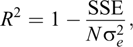
where $σ_{e}^{2}$ is equal to the data variance. Thus, the maximum log-likelihood values and R² values serve as goodness-of-fit measures at the first stage to preselect a number of best fitting models of varying complexity (number of polynomial terms included).

In the second stage of our model selection algorithm, we choose the best model among those obtained in the first stage based on their “robustness.” This stage is necessary because the maximum log-likelihood value increases monotonically with the number of terms, since each term allows an extra degree of freedom on curve fitting. Using maximum log-likelihood values alone for model selection may lead to selecting models with too many terms which fit the existing data accurately but generalize poorly to unseen data and have little predictive power (MacKay 2003; Ranganathan et al. 2014).

To address this problem and evaluate the fit of the six best models selected in the first stage, we adopt a Bayesian model selection approach (Bernardo and Smith 2009; Jaynes 2003; MacKay 2003; Robert 1994; Skilling 2006). We calculate the Bayesian marginal-likelihood (MacKay 2003; Skilling 2006) or the Bayes factor B(m) for the set of models which have the largest log-likelihood value among models with their respective number of terms.

The Bayes factor compensates for the increase in complexity whenever an additional polynomial term is added to the model by integrating over all possible parameter values (MacKay 2003), that is, in our example, for the dY model,

B (m) = \int_{φ (m)} P (d Y | Y, X, φ (m)) π (φ (m)) d φ (m),

where φ(m) is the set of parameters that defines the specific m-term model under consideration. The integration over all possible values of this set of parameters thus means that the Bayes factor is the likelihood value (given a particular value of the parameters) averaged over the parameter space with a prior distribution defined by π(φ(m)). The prior distribution says how likely we thought a particular set of parameter values was before we started the fitting procedure (Bishop 2006).

In our study, we choose a noninformative prior distribution, such that π(φ(m)) is uniform over a range of parameter values. This “noninformative” prior is reasonable when we have no information about the parameter space except its likely range. Since we use Monte Carlo methods to perform the integration, we also need to limit the range of values for φ(m) to include all feasible values but to be small enough for the integral to be computed numerically. Note that the Bayes factor is computationally expensive to calculate. Therefore, we use the two-stage algorithm described above, since models of equal complexity (same number of terms in this context) can be more fairly evaluated in terms of their log-likelihood values. Given the models preselected in the first stage, computing the Bayes factor for these models f(Y, X; φ(m)) with different numbers of terms m is reasonably fast, and we obtain the function B(m). Then, the model with the highest Bayes factor is the model that fits the data best, without overfitting it. As such, the Bayes factor also helps preventing multicollinearity, because a smaller set of uncorrelated polynomial terms is favored by the Bayes factor.

As a result of this model fitting procedure, we arrive at the differential equation that best describes the change dynamics. The parameter estimates of the best fitting differential equation model will all be statistically significant since the Bayes factor is essentially a Bayesian equivalent of significance testing; a model with nonsignificant parameter estimates would have been rejected (Dienes 2011). If no significant effects are detected, the resulting model will be a model, where the changes in the outcome variable are constant (a₀) only.

We can visualize the dynamics described in the derived differential equations in a so-called phase portrait, which shows the coevolution of the two variables over time as suggested by the models, with the vectors representing rates of change in the social system (in our empirical case schools) with specific combinations of Y and X initial values (see Figure 2 for an example). The captured dynamics include acceleration processes, and the phase portrait visualizes the pace through vector arrow lengths: longer arrows mean faster, or accelerated change, shorter arrows mean slower change, with dots indicating absence of change (see Figure 2).

Figure 2.

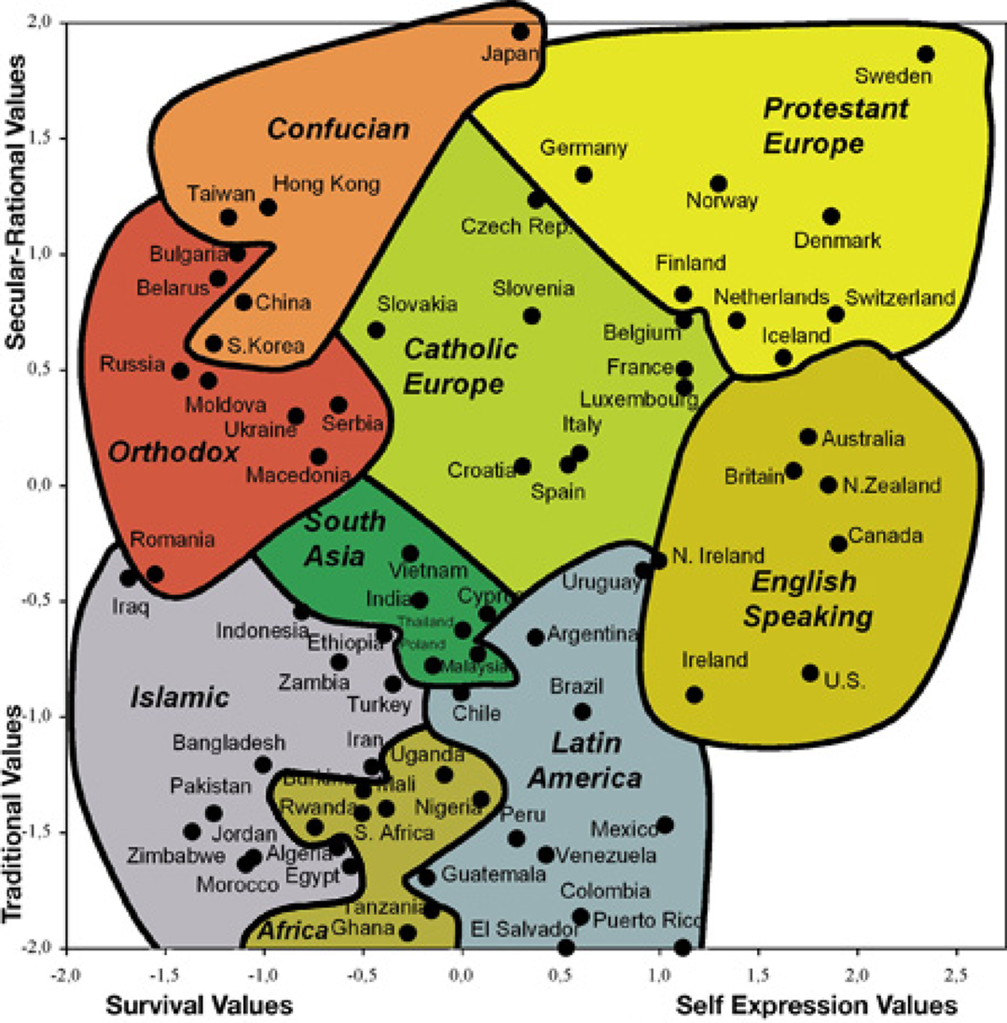
World Values Survey Cultural Map (Inglehart and Welzel 2010:554).

We can also include more variables (X_i). Continuing within the same modeling framework, the function f(Y, X₁, X₂) may now consist of up to 39 different right-hand side terms (Ranganathan et al. 2014). In the two-variable case, the “complexity” of a model depended only on the number of polynomial terms included in the model. When there are three variables, complexity may be measured both in terms of the number of polynomial terms and in terms of the number of explanatory variables included in the model. We use the two-stage algorithm as before but extend it to test if adding other predictors improves the model fit. For instance, in the dY model, we may find that X₂ does not significantly affect changes in Y and hence can be dropped as an explanatory variable. Specifically, the Bayes factor may reveal that the increased model complexity due to the additional predictor X₂ is not sensible in terms of model fitting (Ranganathan et al. 2014).

The discrete data (yearly changes) used in this article would suggest the use of difference equations instead of differential equations. However, we use continuous time models because the underlying social dynamics are mostly continuous, even though the data are not, and doing so provides certain mathematical conveniences. For certain parametrizations, difference equations can produce numerically unstable results when solving the model forward in time. In the models we fit, any such numerical instabilities do not reflect the underlying processes and we therefore assume the variables change smoothly in time, hence the use of differential equations. In most cases, however, it is equally valid to interpret the results in differential as in difference terms.

Data

To demonstrate how our methodological approach can be applied to study complex social system dynamics, we use data from the so-called Stockholm database. This database contains information on all individuals who ever resided in Stockholm county during the years 1990 to 2002. The data are collected from various government registers and includes detailed sociodemographic information. Missing data are almost nonexistent, and the quality of the information is very high.

In Sweden, there are nine years of compulsory education, and this is usually completed between the ages of 7 and 16. In our database, there existed a total of 281 upper secondary schools during the years 1990 to 2002. We focus on the graduating classes of each school, and we use information on the number of students graduating every year, their parents’ countries of birth, their grade point average, and the economic status of their parents. Data availability is the reason for focusing on graduating classes only. This is also the reason why we focus exclusively at the school level in this article. While we can follow schools over long periods of time, we are not able to follow individuals as they move through the school system.

For our main analysis, we used the following four variables:

Proportion of students with Sweden-born parents is denoted by the variable S. The proportion of students within a school whose parents both were born in Sweden measures the presence of the majority group within the school. The rate of change in this variable is the dependent variable in the analyses because it is a key for understanding the segregation dynamics (Caetano and Maheshri 2011, 2013; Card et al. 2006, 2008; Fekjaer and Birkelund 2007).

Perceived foreignness index is denoted by the variable F. Many studies of segregation processes use crude dichotomies between majority and minority groups when measuring the composition of schools, but this obliterates important distinctions between different immigrant groups and their effects on the majority group. A student of Norwegian origin, for example, most likely will be perceived in a different way by students and parents of Swedish origin than would a student of Jordanian background. The Jordanian student would be perceived as more “foreign” than the Norwegian student, and as we know from a range of studies in the homophily tradition (McPherson, Smith-Lovin, and Cook 2001; Wimmer and Lewis 2010), perceptions of similarity are important for attitudes and behavior.

For ease of estimation as well interpretation, we would prefer to have a single variable that takes such country differences into account. We have used results from the World Values Survey to arrive at such a composite proxy variable. More specifically, we combine data from Ingelhart’s so-called cultural map of the world for the 2005 to 2008 period (see Figure 2) with information on the country of birth of the students’ parents. First, we placed the parents of all children in the schools on this map based on their country of birth. Second, we calculated the straight-line distance between Sweden and each parent’s position on the map. For instance, the distance between Sweden and Norway, thus defined, is 0.456 while the distance between Sweden and Jordan is 3.103. Third, each year we calculated the average of these distances for each school, and these averages form the basis of our measure of “perceived foreignness.” The range for the perceived foreignness index in the data is 0 to 2.8.³

Let us emphasize that this index is not intended to properly measure cultural differences. It simply is a proxy for dissimilarity that we think is better at capturing the complexity of people’s perceptions of others than a simple dichotomous categorization of immigrants and nonimmigrants.

Parents’ average income is denoted by the variable I. When calculating the average income of the students’ parents, first we summed the disposable after tax and transfer income of the parents of each child. Then, we used information on family size and number of children to adjust the total disposable income of the family in order to get as good measure as possible of each family’s economic standing. Finally, we calculated the average parental income within each school each year, and the log of this value constitutes our measure. It ranges between 6.0 (around 410,000 Swedish Krona [SEK]/year) and 9.3 (around 11,000,000 SEK/year).

Average grades are denoted by the variable G. We calculated the average grades per year and school on the basis of the students’ average grade in their graduation year. The grading system changed in 1998, and in order to make the grade scores comparable through time, we rescaled the post-1998 grades to make them equivalent to the pre-1998 grades. The range of average grades in the data is 1.2 to 4.7.

Results

We start by examining the relation between two indicators, in our empirical case the perceived foreignness index and the rate of change in the proportion of students with Sweden-born parents. Figure 3 shows how seven randomly selected schools changed position in the space defined by the two indicators over a 12-year period. The dots represent their initial position (usually in 1990) and the lines how they evolved over time. There are some random fluctuations in this data but also some systematic patterns. For example, the black and the brown schools start with similar proportions of students with Sweden-born parents but different perceived foreignness index values. While the black school experiences an increase in the proportion of students with Sweden-born parents, the brown school experiences a decrease. A general trend of schools becoming increasingly ethnically mixed is also visible.

Figure 3.

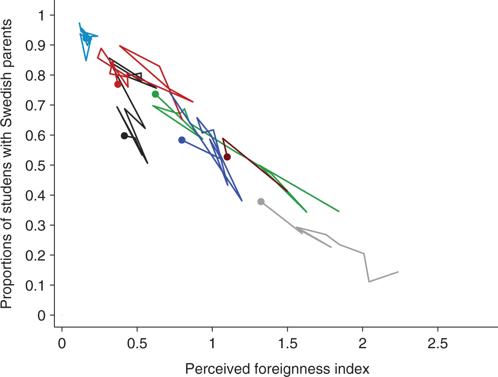
Trajectories of seven randomly selected schools over time in a two-dimensional phase plane defined by S and F.

To systematically identify patterns in this type of data, we fitted equation (5) to the data from all 281 schools. Table 1 summarizes the log likelihood and Bayes factor for the best 1-, 2-, 3-, 4-, and 5-term models, and the model with the highest Bayes factor has four terms:

Table 1.

Model Fits for All Models. Model Fits for the Selected Models in Text (Equations [7], [10], and [12]) Are Highlighted.

Models	Log Likelihood	Bayes Factor
Models with S and F
Equation (7)	−9.4556	−9.4786
$\frac{d S}{d t} = - 0.014 S^{3}$	−9.5578	−9.5408
$\frac{d S}{d t} = 0.045 S^{2} - 0.065 S^{3}$	−9.5461	−9.5501
$\frac{d S}{d t} = 0.196 S - 0.121 S F - 0.214 S^{3}$	−9.5059	−9.4800
$\frac{d S}{d t} = 0.073 F - 0.222 S F + 0.476 S^{2} - 0.493 S^{3} - 0.001 F^{3}$	−9.4453	−9.6179
Models with S, F, and I
Equation (10)	−9.3630	−9.4056
$\frac{d S}{d t} = - 0.014 S^{3}$	−9.5032	−9.5432
$\frac{d S}{d t} = - 0.317 \frac{S}{I} + 0.0005 I^{3}$	−9.4890	−9.5594
$\frac{d S}{d t} = 0.027 I - 1.34 \frac{F}{I} + 0.061 F^{2} - 0.201 S^{3}$	−9.2520	−9.4278
$\frac{d S}{d t} = 0.249 S + 0.6 F - 3.66 \frac{F}{I} - 1.61 \frac{S F}{I} - 0.265 S^{3}$	−9.1749	−9.4209
Models with S, F, and G
Equation (12)	−9.3664	−9.4069
$\frac{d S}{d t} = - 0.014 S^{3}$	−9.5007	−9.5408
$\frac{d S}{d t} = - 0.013 S G + 0.001 G^{3}$	−9.4469	−9.5082
$\frac{d S}{d t} = 0.044 S G - 0.026 S F G - 0.166 S^{3}$	−9.3257	−9.4470
$\frac{d S}{d t} = - 0.088 S - 0.040 S F G + 0.464 S^{2} + 0.006 G^{2} - 0.461 S^{3}$	−9.2175	−9.4072

\frac{d S}{d t} = 0.05 - 0.14 S F + 0.31 S^{2} - 0.37 S^{3} .

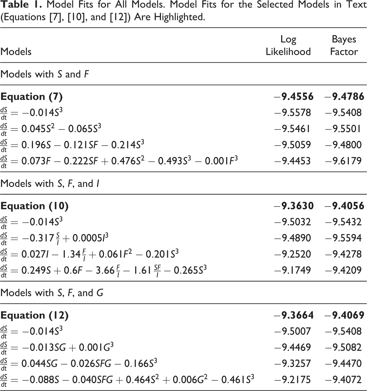
Taking one term at a time, we can understand how these two variables interact. The SF term reveals that perceived foreignness has a negative effect on the rate of change in the proportion of students with Sweden-born parents. The S² term displays a positive feedback loop in regard to the proportions of students with Sweden-born parents, while the negative S³ term represents a self-limiting negative feedback loop, as S approaches its limit at 1.⁴

The estimated model for changes in the perceived foreignness index was much simpler than for changes in the proportion of students with Sweden-born parents. The model

\frac{d F}{d t} = 0.03 S,

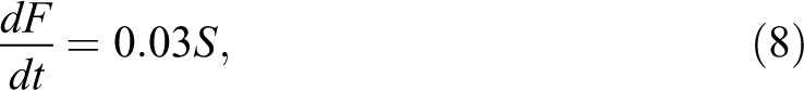
is the one that best fits the data as judged by the Bayes factor. This model tells us that the perceived foreignness index grew on average in the years 1990 to 2002 in all schools, but that it was growing slower in schools with a low proportion of students with Sweden-born parents. We focus in this article on the $\frac{d S}{d t}$ models, because we see changes in the proportion of students with Sweden-born parents as particularly important if we are to understand how the segregation process unfolds. Generally, a dynamical system reveals systematic coevolution of the variables included in the model, which may or may not reflect causality, depending on the relations between the variables in the data. With the two equations (7) and (8), a clear causal interpretation cannot be maintained, we rather see a complex coupling of both indicators and the tipping behavior is a result of this coupling.

The phase portrait (Figure 4a) gives a visual representation of equations (7) and (8) and therefore of the complex dynamics that these equations capture. The figure points to multiple states of the system. Figure 4b shows the predicted trajectories for the seven schools in Figure 3, using the two best fitting differential equations (7) and (8). Comparing the data-based and model-predicted trajectories, we may conclude that our model seems to predict reasonably well the development of various schools in terms of their ethnic composition.

Figure 4.

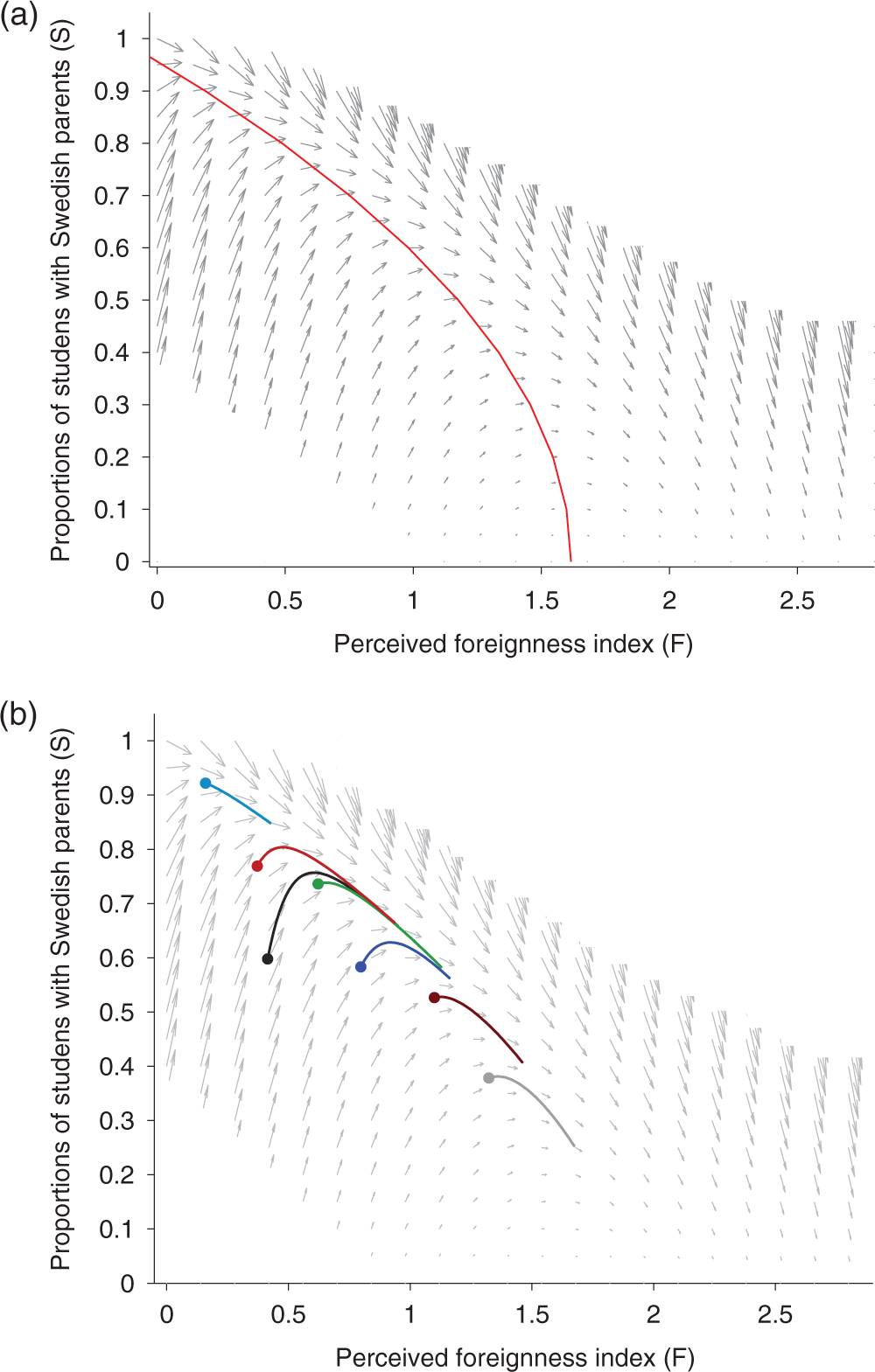
(a) Phase portrait for $\frac{d S}{d t}$ and $\frac{d F}{d t}$ models given by equations (7) and (8) with the red curve visualizing the solutions to the threshold equation (9) and (b) trajectories for the seven randomly selected schools in Figure 3 predicted by the two models (7) and (8), plotted over the phase portrait.

The red curve in Figure 4a represents the set of tipping points. We derived those tipping points by setting equation (7) equal to zero and solving for F_*. This results in the following threshold equation for the perceived foreignness index:

F_{*} = \frac{7.41 (- 0.37 S^{3} + 0.31 S^{2} + 0.05)}{S} .

This threshold equation (red curve in Figure 4a) shows that, in general, schools with a low value on the perceived foreignness index tended to tip toward an increase in the proportion of students with Sweden-born parents, the vectors in Figure 4a point upward. Likewise, schools with high values on the perceived foreignness index tended to tip in the opposite direction, that is, toward a decrease in the proportion of students with Sweden-born parents. It also should be observed that changes in the ethnic makeup of the schools were not simply a function of the proportion of students with Swedish parents. For example, schools at middling levels of S, for example, 70 percent, but with low values on the perceived foreignness variable tended to tip toward larger proportions of students with Sweden-born parents, while those with similar values of S, but higher perceived foreignness tipped in the opposite direction.⁵

Beyond a perceived foreignness index of around 1.5, the proportion of students with Sweden-born parents nearly always tends to decrease. An example is useful to make this pattern easier to understand. A school with a perceived foreignness index of 1.5 could have 65 percent students of Swedish origin, 20 percent of Iranian background, and the rest could consist of small proportions of students from Finland, Middle Europe, South America, and with mixed parental backgrounds. Such a school is highly likely to end up with fewer and fewer students of native Swedish background. In contrast, if the 20 percent were not of Iranian background but of Spanish background, for instance, the perceived foreignness index would be around 0.85 and the school would not tip.

It is often suggested that it is not the ethnic composition that makes the majority group leave, but rather the socioeconomic composition of a school. Because minority groups are often socioeconomically marginalized (Van der Slik, Driessen, and De Bot. 2006; Iceland and Wilkes 2006; Rothstein and Wozny 2011; Sager 2011), the socioeconomic effect may appear as an ethnicity effect. In order to test whether that seems to be the case, we estimated models as those above but which included an additional variable, average parental income (I).

We arrive at the following best fitting model (see also Table 1) for f(S, F, I):

\frac{d S}{d t} = 0.03 S (I - 29.33 \frac{F}{I} - 8.33 S^{2}) .

Like equation (7), this equation includes a negative effect of F on changes in S. It also has a self-limiting negative feedback of S on itself. The multiplicative I term indicates that schools with wealthier parents experience larger increases in students with Sweden-born parents.⁶ From equation (10), we can also derive the threshold equation:⁷

F_{*} = 0.04 I (I - 9.33 S^{2}) .

Figure 5 displays various tipping point curves based on equation (11), solved with different values for S and I. The curves show how the tipping points depend on the level of parental income I.⁸ The dashed red curve is the solution to the original threshold equation (9), that is, when not taking parents’ average income into account. Figure 5 reveals how parents’ average income moves the set of tipping points. There is a general tendency for schools with high parental income to have higher tipping points, thus the set of tipping points is moved to the right from the original tipping point curve (dashed red curve). The effect of parents’ income on the perceived foreignness index tipping points decreases slightly for schools with high proportions of Sweden-born parents (i.e., the curves in Figure 5 for large S are closer together).⁹

Figure 5.

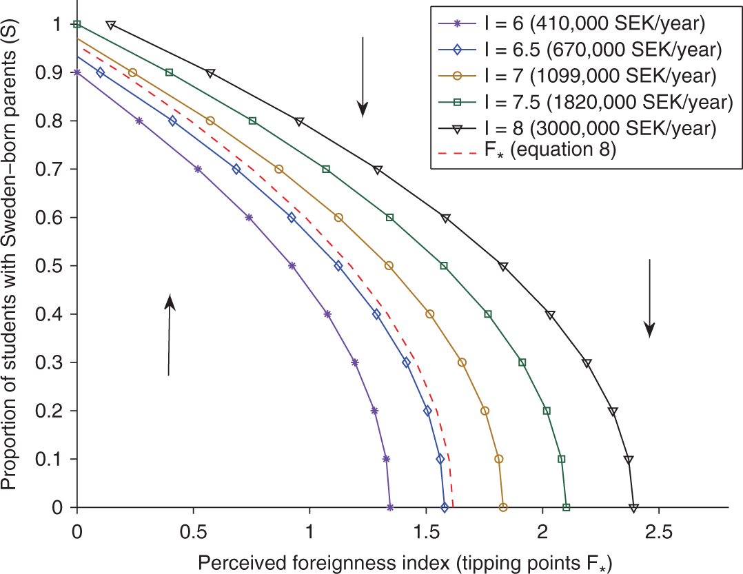
Perceived foreignness index tipping points for various initial conditions for proportion of students with Sweden-born parents S [0–1] and average parents’ income I [6–8]. The red dashed curve represents the F_* curve in Figure 4a and therefore the solutions to equation 9. The arrows indicate the regions where S is either expected to increase or decrease.

Another factor that could be of potential importance is the quality of the school, which we approximated with average grades (G). The following was the best fitting model (see Table 1) for f(S, F, G):

\frac{d S}{d t} = 0.3 S (S - 1.267 S^{2}) + 0.01 G (G - 4 S F) .

Again, we see a combination of reinforcement of S on itself, combined with a self-limiting feedback. The quadratic positive G term suggests that schools with high average grades tend to get increasing proportions of students with Sweden-born parents. The three-way interaction term −SFG shows that the effect of grades is reduced in schools, where the perceived foreignness index is high.

Once grades are included in the analysis, the threshold equation becomes:¹⁰

F_{*} = \frac{22.68 (0.30 S^{2} + 0.005 G^{2} - 0.38 S^{3})}{S G} .

Solutions to the threshold equation (13) with various values for S and G are visualized in Figure 6. In general, schools with higher average grades are less likely to experience decreases in the number of students with Sweden-born parents. This pattern is most pronounced when S is low and F is high. When the grades in the school are average or above, then the number of students with Sweden-born parents reaches a stable equilibrium. If the grades are low, however, schools with high values on the perceived foreignness index will experience decreases in students with Sweden-born parents (as was the case for equation [9]).

Figure 6.

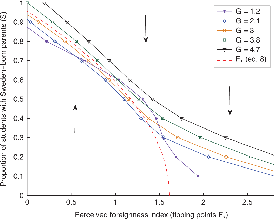
Perceived foreignness index tipping points for various proportions of students with Sweden-born parents S [0–1] and average grades G [1.2–4.7]. The red dashed curve represents the F_* curve in Figure 4a and therefore the solutions to equation (9). The arrows indicate the regions where S is either expected to increase or decrease.

We also estimated models with all four indicators, S, F, I, and G, thus f(S, F, I, G). The best overall model was again equation (10), with a Bayes factor of −9.4056. The fact that the best model does not contain G as predictor tells us, that including all four predictors does not result in a better model. Ultimately, income of parents is a better predictor of changes in the proportion of students with Sweden-born parents than are average grades. This result reminds us to interpret Figure 6 with caution. While increasing grades do appear to move the tipping point upward, the evidence for this is not as strong as for parents’ income.

Finally, we also included neighborhood characteristics (neighborhood proportion of native Swedes and neighborhood perceived foreignness index) in our analysis. Earlier studies (Bergsten 2010; Brännström 2008; Kauppinen 2008; Östh, Andersson, and Malmberg 2013) have already suggested that school segregation is strongly coupled with neighborhood segregation. Our analyses confirm these findings and show that both types of segregation phenomena influence each other without a clear causal ordering (see Appendix Table A1). However, the correlation between school and neighborhood segregation is far from perfect (see Appendix Figure A1). This suggests that although schools’ ethnic composition resembles strongly neighborhood ethnic composition, and although we find equivalent segregation dynamics in the neighborhoods as in the schools (see fifth row in the Appendix Table A1), there are also endogenous dynamics in both the schools and the neighborhoods.

Discussion

Identifying complex dynamics and interactions is important if we are to understand how complex processes in social systems, such as segregation, unfold. Identifying complex patterns like tipping points or multiple phase transitions contributes to our understanding of what triggers big and often abrupt changes in social systems. From a more practical point of view, the identification of complex dynamics enables us to make predictions for concrete cases, for instance for the segregation of specific schools (see Figure 4b). Such knowledge is important for the design of efficient policy interventions.

Recently, Lamberson and Page (2012:177) have argued for the importance of using the “mathematical formalism of dynamical systems to define tipping points as discontinuities in the relationship between present conditions and future states of the system”. In this article, we have responded to this call by proposing a dynamical systems approach. We demonstrated how to use this approach with empirical data in order to identify complex nonlinear social system dynamics, such as tipping and multiple phase transitions. More specifically, we used Swedish register data to empirically identify multiple thresholds in Swedish schools in terms of their perceived foreignness and analyzed how these thresholds depend upon the proportion of students with Sweden-born parents in the school, the quality of the schools, and the income of the parents.

Our results confirm earlier studies based on micro-level data which have suggested that the ethnic and socioeconomic composition of schools and school quality are important school choice criteria. However, our approach also reveals nonlinear systemic patterns and complex interactions. Ethnically mixed schools lead to a rapid decrease in the proportion of Swedish students only once the perceived foreignness index of a school reaches a critical level. The critical threshold itself however varies with different factors. For instance, ethnically mixed schools are less affected by a downward trend in the proportion of Swedish students if the (immigrant) students have a rather affluent background or if the ethnically mixed schools are high performing schools.

When interpreting the results it is important to distinguish between segregation dynamics and schools becoming increasingly ethnically diverse. Our empirical analyses allowed for models with trend terms (intercepts) and the fact that we nevertheless found that the best fitting models included terms that indicated tipping-like behavior suggests that endogenous segregation dynamics were indeed important. We also would like to emphasize once more that the models should not be interpreted in strictly causal terms. Even though the dynamics we analyze have a temporal pattern, the causal direction of these patterns is not always clear, since the indicators and therefore their effects seem to be coupled and mutually reinforcing and interdependent. Moreover, as mentioned in the introduction, our data did not provide any variables that could serve as instrumental variables, which calls for even more caution when making any causal inferences. But, causality is not necessarily always the best way to understand system dynamics, in fact, studying the complex coupling of various phenomena and the nonlinear effects this coupling may have, can provide important and useful explanations of the processes through which changes in social systems are brought about.

We do not seek to generalize our substantive findings beyond the actual set of schools being analyzed. With John Goering’s words: “[…] there is nothing necessarily predetermined or inevitable about these shifts [tipping points]” (2013:14). The aim of the article has been to provide methods for capturing complex empirical dynamics that lead to phase transitions and discontinuities in social systems such as schools. Focusing on state changes in the social system is one way to study complex dynamics. Another approach would be to study changes in the flows of students between schools, that is to model dynamical flows and not dynamical systems change. This latter approach would have required individual-level panel data however.

Ultimately, we think that both types of approaches can generate novel insights that help us to better understand the dynamics and mechanisms at work. Whenever possible, it is preferable to perform both types of analyses and to compare the results with one another. Moreover, having identified the crucial dynamics observed on the macro level and the mechanisms at the micro level we can take the next step and try to systematically link both levels to one another, for instance, by developing agent-based models based on the empirical results.

The method detailed in this article is applicable to a wide range of phenomena. Complex, nonlinear phenomena appear in all social systems on all aggregation levels. Political transitions, economic development, and sociocultural changes may be analyzed using this approach (Anderies 2003; Spaiser et al. 2014) as well as social conflicts (Coleman, Vallacher, and Nowak 2007) or socioeconomic changes in cities, neighborhoods, schools, or working places (Batty 1971; White, Engelen, and Uljee 2015). The method is moreover highly flexible in response to the specific research requirements, that is, we could include instrumental variables and increase time lags in order to be able to make stronger causal claims. It is also possible to include linear control variables in the models that would not serve the purpose of identifying complex interactions, but would allow for controlling for various factors that are not of primary interest. Various types of stochasticity can be additively implemented as well. This is of particular interest if the models are to be used for making predictions about changes in the social system (Ranganathan et al. 2015). And the mathematical models derived from the data can be used to explore various social or political scenarios involving the social system (Ranganathan and Swain 2014; Strulik 1999). Finally, the set and type of polynomial terms defined in equation (5) can be easily changed as well, either reduced to specific terms that for instance represent specific theoretical assumptions or extended to include other polynomial terms, if there is reason to assume that such an extension is necessary to represent certain patterns in the data. As such, our methodological approach can be seen as a flexible toolbox; a potentially important addition to other approaches, suitable for analyzing social system dynamics.

Footnotes

Declaration of Conflicting Interests

The author(s) declared no potential conflicts of interest with respect to the research, authorship, and/or publication of this article.

Funding

The author(s) disclosed receipt of the following financial support for the research, authorship, and/or publication of this article: The authors received financial support for the research and publication of this article by the European Research Council, ERC grant agreement no. 324233, Riksbankens Jubileumsfond and Vetenskaprådet project grant 2013: Development Space.

Supplemental Material

Supplementary material for this article is available online.

Notes

References

Anderies

John M.

2003. “Economic Development, Demographics, and Renewable Resources: A Dynamical Systems Approach.” Environment and Development Economics 8:219–46.

Andersson

Eva

Malmberg

Östh

John

. 2012. “Travel-to-school Distance in Sweden 2000-2006: Changing School Geography with Equality Implications.” Journal of Transport Geography 23:35–43.

Andersson

Eva

Östh

John

Malmberg

. 2010. “Ethnic Segregation and Performance Inequality in the Swedish School System: A Regional Perspective.” Environment and Planning A 42:2674–86.

Andrey

Andreev

Borodkin

Leonid

Levandovskii

Mikhail

. 1997. “Using Methods of Non-linear Dynamics in Historical Social Research: Application of Chaos Theory in the Analysis of the Worker’s Movement in Pre-revolutionary Russia.” Historical Social Research 22:64–83.

Batty

Michael

. 1971. “Modelling Cities as Dynamic Systems.” Nature 231:425–28.

Bergsten

Zara

. 2010. Battre framtidsutsikter? Blandade bostadsområden och grannskapseffekter: en analys av visioner och effekter av blandat boende. Uppsala, Sweden: Department of Social and Economic Geography, Uppsala University.

Bernardo

Jose M.

Smith

Adrian F. M.

. 2009. Bayesian Theory. Chichester, UK: John Wiley & Sons.

Bishop

Christopher M.

2006. Pattern Recognition and Machine Learning. New York: Springer.

Bossel

Hartmut

. 1994. Modeling and Simulation. Wiesbaden, Germany: Vieweg.

10.

Bowden

Roger J.

Turkington

Darrell A.

. 1990. Instrumental Variables. Cambridge, UK: Cambridge University Press.

11.

Brännström

Lars

. 2008. “Making Their Mark: The Effects of Neighbourhood and Upper Secondary School on Educational Achievement.” European Sociological Review 24:463–78.

12.

Bunar

Nihad

. 2010. “The Geographies of Education and Relationships in a Multicultural City.” Acta Sociologica 53:141–59.

13.

Bunar

Nihad

Kallstenius

Jenny

. 2005. I min gamla skola lärde jag mig fel svenska. En studie om skolvalfrihet i det polariserade urbana rummet. Stockholm, Sweden: Integrationsverket.

14.

Burgess

Simon

McConnell

Brendon

Propper

Carol

Wilson

Deborah

. 2005. The Impact of School Choice on Sorting by Ability and Socio-economic Factors in English Secondary Education. CMPO, University of Bristol. Bristol, UK.

15.

Butler

Tim

Hamnett

Chris

Ramsden

Mark

Webber

Richard

. 2007. “The Best, the Worst and the Average: Secondary School Choice and Education Performance in East London.” Journal of Education Policy 22:7–29.

16.

Caetano

Gregorio

Maheshri

Vikram

. 2011. “School Segregation and the Identification of Tipping Points.” Working Paper, University of Rochester, Rochester, NY.

17.

Caetano

Gregorio

Maheshri

Vikram

. 2013. “School Segregation and the Identification of Tipping Behavior.” Working Paper 2013-252-50, University of Houston, Houston, TX.

18.

Caetano

Gregorio

Maheshri

Vikram

. 2015. “School Segregation and the Identification of Tipping Behavior.” Working Paper, University of Houston. Accessed March 21, 2015. Retrieved (http://www.gregoriocaetano.net/resources/Research/caetano_maheshri_tipping.pdf).

19.

Campbell

David K.

Mayer-Kress

Gottfried

. 1997. “Chaos and Politics: Application of Non-linear Dynamics to Socio-political Issues.” In The Impact of Chaos on Science and Society, 18–63 edited by Grebogi

Celso

Yorke

James A.

. Tokyo, Japan: United Nations University Press.

20.

Card

David

Mas

Alexander

Rothstein

Jesse

. 2006. “Tipping and the Dynamics of Segregation in Neighborhoods and Schools.” Working Paper, University of California, Berkeley.

21.

Card

David

Mas

Alexander

Rothstein

Jesse

. 2008. “Tipping and the Dynamics of Segregation.” The Quarterly Journal of Economics 123:177–218.

22.

Coleman

Peter T.

Vallacher

Robin R.

Nowak

Andrzej

. 2007. “Intractable Conflict as an Attractor. A Dynamical Systems Approach to Conflict Escalation and Intractability.” American Behavioural Scientist 50:1454–75.

23.

de Vries

Bert J. M.

2013. Sustainability Science. Cambridge, UK: Cambridge University Press.

24.

DeSena

Judith N.

2006. “What’s a Mother to Do?” American Behavioral Scientist 50:241–57.

25.

Dienes

Zoltan

. 2011. “Bayesian versus Orthodox Statistics: Which Side Are You On?” Perspectives of Psychological Science 6:274–90.

26.

Fekjaer

Silje N.

Birkelund

Gunn E.

. 2007. “Does the Ethnic Composition of Upper Secondary Schools Influence Educational Achievement and Attainment? A Multilevel Analysis of the Norwegian Case.” European Sociological Review 23:309–23.

27.

Goering

John

. 1978. “Neighborhood Tipping and Racial Transition.” Journal of the American Institute of Planners 44:68–78.

28.

Goering

John

. 2013. “Neighborhood Effects and Public Policy.” City & Community 12:13–20.

29.

Granovetter

Mark

Soong

Roland

. 1988. “Threshold Models of Diversity: Chinese Restaurants, Residential Segregation and the Spiral of Silence.” Sociological Methodology 18:69–104.

30.

Grodzins

Morton

. 1957. “Metropolitan Segregation.” Scientific American 197:33–41.

31.

Grodzins

Morton

. 1958. Government and Housing in Metropolitan Areas. New York: McGraw Hill.

32.

Hatt

Ken

. 2009. “Considering Complexity: Toward a Strategy for Non-linear Analysis.” Canadian Journal of Sociology 34:313–47.

33.

Hedström

Peter

. 2005. Dissecting the Social: On the Principles of Analytical Sociology. Cambridge, UK: Cambridge University Press.

34.

Iceland

John

Wilkes

Rima

. 2006. “Race, Class and Residential Segregation.” Social Problems 53:248–73.

35.

Inglehart

Ronald

Welzel

Christian

. 2010. “Changing Mass Priorities: The Link between Modernization and Democracy.” Perspectives on Politics 8:551–67.

36.

Jackson

Matthew O.

Yariv

Leeat

. 2007. “Diffusion of Behavior and Equilibrium Properties in Network Games.” American Economic Review 97:92–98.

37.

Jaynes

Edwin T.

2003. Probability Theory: The Logic of Science. Cambridge, UK: Cambridge University Press.

38.

Jervis

Robert

. 2009. “Black Swans in Politics.” Critical Review 21:475–89.

39.

Johansson

Thomas

Hammarén

Nils

. 2010. “Konsten att välja rätt spårvagn. En studie av segregation, skolval och unga människors studieplaner.” Sociologisk forskning 47:51–71.

40.

Karsten

Sjoerd

Ledoux

Guuske

Roeleveld

Jaap

Felix

Charles

Elshof

Dorothé

. 2003. “School Choice and Ethnic Segregation.” Educational Policy 17:452–77.

41.

Kauppinen

Timo M.

2008. “Schools as Mediators of Neighbourhood Effects on Choice between Vocational and Academic Tracks of Secondary Education in Helsinki.” European Sociological Review 24:379–91.

42.

Lamberson

P. J.

Page

Scott E.

. 2012. “Tipping Points.” Quarterly Journal of Political Science 7:175–208.

43.

Qui

Racine

Jeffrey Scott

. 2007. Nonparametric Econometrics: Theory and Practice. Princeton, NJ: Princeton University Press.

44.

Lindbom

Anders

. 2010. “School Choice in Sweden: Effects on Student Performance, School Costs, and Segregation.” Scandinavian Journal of Educational Research 54:615–30.

45.

Lindbom

Anders

Almgren

Ellen

. 2007. “Valfrihetens effecter på skolornas elevsammansättning: Skolsegreation i Sverige.” In Friskolorna och framtiden—segregation, kostnader och effektivitet, 89–118 edited by Lindbom

Anders

. Stockholm, Sweden: Institutet för framtidsstudier.

46.

MacKay

David J. C.

2003. Information Theory, Inference and Learning Algorithms. Cambridge, UK: Cambridge University Press.

47.

McPherson

Miller

Smith-Lovin

Lynn

Cook

James M.

. 2001. “Birds of a Feather: Homophily in Social Networks.” American Review of Sociology 27:415–44.

48.

Meadows

Donella H.

2008. Thinking in Systems. West River Junction, VT: Chelsea Green.

49.

Meuleman

Bart

Davidov

Eldad

Billiet

Jaak

. 2009. “Changing Attitudes toward Immigrant in Europe, 2002-2007: A Dynamic Group Conflict Theory Approach.” Social Science Research 38:352–65.

50.

Noreisch

Kathleen

. 2007. “School Catchment Area Evasion: The Case of Berlin.” Journal of Education Policy 22:69–90.

51.

Östh

John

Andersson

Eva

Malmberg

. 2013. “School Choice and Increasing Performance Difference: A Counterfactual Approach.” Urban Studies 50:407–25.

52.

Pancs

Romans

Vriend

Nicolas J.

. 2007. “Schelling’s Spatial Proximity Model of Segregation Revisited.” Journal of Public Economics 91:1–24.

53.

Quercia

Roberto

Galster

George

. 2000. “Threshold Effects and Neighborhood Change.” Journal of Planning Education and Research 20:146–62.

54.

Ranganathan

Shyam

Swain

Ranjula Bali

. 2014. “Setting Sustainable Development Goals—A Dynamical Systems Approach.” Working Paper No. 491, Stanford Center for International Development, Stanford, CA.

55.

Ranganathan

Shyam

Nicolis

Stamatios C.

Spaiser

Viktoria

Sumpter

David J. T.

. 2015. “Understanding Democracy and Development Traps Using a Data-driven Approach.” Big Data 3:22–33.

56.

Ranganathan

Shyam

Spaiser

Viktoria

Mann

Richard P.

Sumpter

David J. T.

. 2014. “Bayesian Dynamical System Modelling in Social Sciences.” PLOS One 9:e86468. doi: 10.1371/journal.pone.0086468.

57.

Reay

Diane

. 2004. “Exclusivity, Exclusion, and Social Class in Urban Education Markets in the United Kingdom.” Urban Education 39:537–60.

58.

Richardson

George P.

1991. Feedback Thought in Social Science and System Theory. Philadelphia: University of Pennsylvania Press.

59.

Robert

Chistian P.

1994. The Bayesian Choice: A Decision-theoretic Motivation. New York: Springer.

60.

Rothstein

Jesse

Wozny

Nathan

. 2011. “Permanent Income and the Black-white Test Score Gap.” NBER (National Bureau of Economic Research Inc.) Working Papers 17610, Cambridge, MA.

61.

Sager

Lutz

. 2011. “Residential Segregation and Socioeconomic Neighbourhood Sorting: Evidence at the Micro-neighbourhood Level for Migrant Groups in Germany.” Urban Studies 49:2617–32.

62.

Saporito

Salvatore

Lareau

Annette

. 1999. “School Selection as a Process: The Multiple Dimensions of Race in Framing Educational Choice.” Social Problems 46:418–39.

63.

Schafer

Chelsea E.

Shaw

Greg M.

. 2009. “Trends—Tolerance in the United States.” Public Opinion Quarterly 73:404–31.

64.

Schelling

Thomas C.

1969. “Models of Segregation.” American Economic Review 59:488–93.

65.

Schelling

Thomas C.

1971. “Dynamic Models of Segregation.” Journal of Mathematical Sociology 1:143–86.

66.

Sethi

Raijv

Somanathan

Rohini

. 2004. “Inequality and Segregation.” Journal of Political Economy 112:1296–321.

67.

Skilling

John

. 2006. “Nested Sampling for General Bayesian Computation.” Bayesian Analysis 1:833–59.

68.

Skolverket. 2006. “Vad händer med likvärdigheten i svensk skola?” Skolverket Report, Stockholm, Sweden.

69.

Söderström

Martin

Uusitalo

Roope

. 2010. “School Choice and Segregation: Evidence from an Admission Reform.” The Scandinavian Journal of Economics 112:55–76.

70.

Sole

Richard V.

2011. Phase Transitions. Princeton, NJ: Princeton University Press.

71.

Spaiser

Viktoria

Ranganathan

Shyam

Mann

Richard P.

Sumpter

David J. T.

. 2014. “The Dynamics of Democracy, Development and Cultural Values.” PLOS One 9:e97856. doi: 10.1371/journal.pone.0097856.

72.

Strulik

Holger

. 1999. “Demographic Transition, Stagnation, and Demoeconomic Cycles in a Model for the Less Developed Economy.” Journal of Macroeconomics 21:397–413.

73.

Trumberg

Anders

. 2011. “Den delade skolan. Segregationsprocesser i det svenska skolsystemet.” Working Paper, Örebro University, Örebro, Sweden.

74.

Utbildnings och kulturdepartementet. 2006. “Likvärdighet i utbildningen.” Utbildnings-och kulturdepartementet Report, Stockholm, Sweden.

75.

Van der Slik

W. P. Frans

Driessen

Geert W. J. M.

De Bot

Kees L. J.

. 2006. “Ethnic and Socioeconomic Class Composition and Language Proficiency: A Longitudinal Multilevel Examination in Dutch Elementary Schools.” European Sociological Review 22:293–308.

76.

White

Roger

Engelen

Guy

Uljee

Inge

. 2015. Modelling Cities and Regions as Complex Systems. From Theory to Planning Applications. Cambridge, MA: MIT Press.

77.

Wimmer

Andreas

Lewis

Kevis

. 2010. “Beyond and Below Racial Homophily: ERG Models of a Friendship Network Documented on Facebook.” American Journal of Sociology 116:583–642.

78.

Zambelli

Stefano

George

Donald A. R.

. 2012. Nonlinearity, Complexity and Randomness in Economics: Towards Algorithmic Foundations for Economics. West Sussex, UK: Wiley-Blackwell.

79.

Zhang

Junfu

. 2009. “Tipping and Residential Segregation: A Unified Schelling Model.” Journal of Regional Science 51:167–93.

Supplementary Material

Please find the following supplemental material available below.

For Open Access articles published under a Creative Commons License, all supplemental material carries the same license as the article it is associated with.

For non-Open Access articles published, all supplemental material carries a non-exclusive license, and permission requests for re-use of supplemental material or any part of supplemental material shall be sent directly to the copyright owner as specified in the copyright notice associated with the article.

0.00 MB

0.14 MB

Identifying Complex Dynamics in Social Systems

Abstract

Keywords

Introduction

Complex Dynamics, Tipping, and Segregation Dynamics

Data and Methods

Methods

Data

Results

Discussion

Footnotes

Declaration of Conflicting Interests

Funding

Supplemental Material

Notes

References

Supplementary Material