An Innovative Approach to Predict Drinking Water Risks Using System,Community,and Regulatory Characteristics

Abstract

Robust predictive models are essential for preventing and mitigating risks associated with public drinking water systems (PWS), which pose significant public health threats and incur substantial medical costs. This study introduces a novel approach by comparing the performance of Logit, Support Vector Machine (SVM), and Extreme Gradient Boosting (XGBoost) models in predicting risks based on PWS characteristics, community attributes, and regulatory developments, rather than relying on water quality and hydrological parameters. The study yields 3 key findings: (1) XGBoost outperforms Logit and SVM, though all models perform less effectively for predicting health-based risks; (2) community and regulatory characteristics exert a greater influence on risk predictions than PWS characteristics; and (3) XGBoost performs comparably to the water parameter-based prediction approach, with the added benefits of lower cost and suitability for long-term forecasting. This innovative approach offers substantial potential for residents, environmental advocates, and policymakers to better anticipate and address PWS risks by focusing on fundamental social determinants.

• ■ A novel approach for predicting U.S. public drinking water system (PWS) risks using system, community, and regulatory characteristics.

• ■ XGBoost outperforms Logit and SVM models in risk prediction.

• ■ XGBoost achieves comparable performance to the water quality and hydrological parameter-based prediction approach.

• ■ Community and regulatory characteristics have a greater impact on risk predictions than PWS characteristics.

Introduction

Robust predictive models are essential for preventing and preparing for risks associated with public drinking water systems (PWS), which are estimated to cause millions of illnesses and incur billions of dollars in healthcare costs annually in the United States.^{1 -4} These risks arise when a PWS violates standards and regulations set by the Environmental Protection Agency (EPA) under the Safe Drinking Water Act (SDWA), such as exceeding allowable contaminant levels or failing to conduct required testing, corrective actions, or timely public notifications.

Prior studies have predominantly relied on water quality and hydrological data from sensors and laboratory experiments to predict drinking water quality or risks. First, time series data on variables such as pH, dissolved oxygen, conductivity, turbidity, Chemical Oxygen Demand, Ammonia Nitrogen, water temperature, and microbial concentrations at the water intake, along with upstream precipitation data, were used to predict drinking water quality or associated risks.^5,6 Second, cross-sectional data on these parameters - along with disinfection byproducts, bacterial abundances, total hardness, total dissolved solids, pipe materials and distribution, traffic conditions, water age, disaster risks and recovery efforts, and seasonal climatic variations – were used to predict various outcomes, including contamination events, drinkability, disaster-related damage to PWS water production, groundwater quality, drinking water production capacity (ensuring compliance with quality standards or minimizing risks), and pipe failure risk.^{7 -14}

However, few studies have investigated the potential for predicting these risks using the characteristics of PWS, the service communities, and regulatory developments. Drinking water protection occurs within specific social contexts, which may play a more fundamental role than water quality or hydrological parameters in contributing to or predicting drinking water risks. In fact, social and regulatory development factors are increasingly recognized as fundamental determinants that influence the necessity, prioritization, and level of investment in PWS construction and maintenance, water quality monitoring, rectification of PWS violations, and mitigation of health-related problems.^{15 -19} For example, in economically disadvantaged or minority-concentrated communities in the United States, the social context directly and indirectly affects whether the population has the financial resources, political power, and other means to build new PWS, improve infrastructure, monitor water quality, and secure governmental support.^{15,20 -25}

Increasing evidence shows that the characteristics of PWS, service communities, and regulatory developments are closely associated with drinking water quality and risks. Larger PWS in urban areas generally experience fewer environmental violations compared to smaller systems in rural regions,^{1,21,26 -28} where greater reliance on groundwater and agricultural land use is often linked to higher nitrate levels in drinking water. ²⁵ Moreover, economically disadvantaged communities are disproportionately exposed to higher levels of arsenic, nitrate, and lead,^25,26,29 while having lower levels of total trihalomethanes.^22,30 Latino communities are particularly vulnerable to elevated nitrate and arsenic exposure,^26,29,31 whereas African American communities tend to have lower nitrate levels. ²⁵ Economically disadvantaged and minority-concentrated communities also face more frequent PWS environmental violations and experience delays in environmental enforcement due to inadequate monitoring, public education, and regulatory oversight.^{15,23,24,32 -34} Inadequate regulatory oversight – particularly in rural areas – may involve insufficient monitoring of drinking water, delayed government responses to violations, limited environmental health interventions, and weak enforcement of sanctions.^23,24

Additionally, the dynamics of socio-political structures can significantly impact PWS risks. ¹⁵ For instance, the 2014 drinking water crisis in Flint, Michigan, highlighted how differing partisan control across levels of government exacerbated these risks. Specifically, higher-level governments with differing partisan representation prioritized fiscal concerns over public health, leveraging mechanisms such as local government takeovers, influencing resource allocation, and blurring lines of accountability, all within the context of the growing financial precarity faced by many U.S. cities.^{35 -41}

PWS risk predictions based on these characteristics are likely more cost-effective and better suited for long-term forecasting compared to those based on water parameter data. Collecting water parameter data typically requires expensive sensors and equipment for continuous monitoring, ⁴² while data on community and regulatory characteristics are readily available from sources such as census datasets or social surveys. Since these social and regulatory factors tend to change gradually, they provide a more stable foundation for long-term risk prediction. A useful metaphor to illustrate the differences between these 2 approaches is predicting college entrance exam outcomes. Predictions based on water parameter data are similar to using mock exam results to forecast final exam outcomes, offering immediate but short-term insights. In contrast, predictions based on these characteristics are analogous to forecasting the outcome using family background, school quality, and educational policies – factors that change gradually and provide a more stable, long-term perspective.

This study aims to develop 3 types of models based on these characteristics to predict PWS risks, compare their predictive performance to models based on water parameters, and analyze the contributions of characteristic variables to the risks. This study offers a more fundamental, cost-effective approach that is also suitable for long-term forecasting in predicting drinking water risks, not an exercise of data analysis. Practitioners and residents can leverage available social and regulatory development data, instead of relying on costly monitoring equipment, to predict and prepare for risks. Regulators can also utilize these models to more effectively implement policies, allocate resources, and empower communities to mitigate and manage risks. The following sections first introduce the data sources, variables, and predictive models, followed by a comparison of model performance and an analysis of variable contributions.

Data and Methods

Data

The research workflow begins with integrating PWS and social data in Subsections 2.1 and 2.2, continues with developing 3 predictive models for PWS risks in Subsection 2.3, and concludes with a comparative evaluation of these models in Subsection 2.4 and 2.5 (see Figure 1).

Figure 1.

Research workflow for comparing models predicting PWS risks.

We focus on Michigan PWS to minimize variations in political institutions and hydrogeological factors across U.S. states. Using the EPA’s Enforcement and Compliance History Online (ECHO) database, we obtained approximately 187 050 environmental enforcement records for Michigan PWS from January 1978 to March 2023. After removing 34 500 duplicate records, 2054 records with missing key violation information, and 87 370 follow-up inspection records, we merged the remaining 63 126 records with census data by aligning each PWS to the most appropriate geographical boundary of a census place. Specifically, records for Community Water Systems (CWS) were merged with socio-economic data from census places of similar population sizes (within a population ratio range of 70%-130%), while records for Transient Noncommunity Water Systems (TNCWS) and Nontransient Noncommunity Water Systems (NTNCWS) were merged with county subdivision socio-economic data, as these systems are managed directly or indirectly by county subdivision governments. Ultimately, over 98% of the records were merged with county subdivision-level data, while the remaining records were merged with either county-level or census tract-level data.

These data were further combined with state governor’s partisan association data (using year as the key variable), county-level presidential support data (using geographic location as the key variable), and drinking water regulatory development data (also using year as the key variable; see Appendix 1). We utilized county-level presidential support data to represent the socio-political structure of each county, as data on the partisan affiliations of county-level governors and county-subdivision leaders were unavailable. Each partisan association, presidential support, and regulatory category was coded as a binary variable; for instance, National Primary Drinking Water Standards (NPDWR85) is coded as 1 for records from 1985 to 2023, and 0 for records from 1978 to 1984, prior to its enactment.

Variables

The outcome variable is PWS risks, classified by the EPA into 4 categories using 3 key indicators: IS_HEALTH_BASED_IND, IS_MAJOR_VIOL_IND, and CALCULATED_PUB_NOTIF_TIER. The risk categories are defined as follows: (1) Major health-based risks (Major risks (H)): contaminants posing immediate risks, requiring public notification within 24 h, due to violations of treatment technique requirements (TT) or exceedances of maximum contaminant levels (MCL) or maximum residual disinfectant levels (MRDL); (2) Minor health-based risks (Minor risks (H)): contaminants violating TT or exceeding MCL or MRDL without immediate risks, requiring public notification within 30 days; (3) Major non-health-based risks (Major risks (N)): major Monitoring and Reporting (MR) violations without TT violations or MCL/MRDL exceedances; and (4) Minor non-health-based risks (Minor risks (N)): minor MR violations without TT violations or MCL/MRDL exceedances. These categorical risk levels provide a more holistic assessment of each PWS’s health risks than individual contaminant concentrations or monitoring and reporting violations. In 2024, the EPA regulated 92 contaminants with varying toxicological thresholds and multiple types of monitoring and reporting requirements. However, the absence of a standardized drinking water quality index makes it impractical to use these disparate metrics to quantify overall PWS health risk in research.

Independent variables (features) include characteristics of the PWS, the service community, and regulatory development. PWS characteristic variables include environmental enforcement bodies, PWS types and ownership, water sources, grant eligibility, wholesaler status, and service to daycares or schools (see Table 2). Service community characteristic variables include population size, number of service connections, median household income, poverty rates, educational attainment, racial and ethnic demographics, workforce proportions, governor’s partisan association, and county-level presidential support (see Table 3). Regulatory development was depicted in 18 binary variables representing drinking water regulations enacted since 1974 (see Appendix 1). Median household income is adjusted to 1999 U.S. dollars using the Consumer Price Index, and all continuous variables are standardized before being incorporated into the models.

Notably, the outcome variable reflects contaminant concentrations and the severity of monitoring and reporting issues in treated water from PWS. While the independent variables include 5 types of drinking water sources, they do not incorporate water quality or hydrological parameters of source water due to regulatory and data limitations. EPA and state agencies require PWS to monitor source water for Cryptosporidium, E. coli, and turbidity only during the initial determination of treatment requirements. PWS that implement maximum treatment are exempt from ongoing source water monitoring. Therefore, these limited and non-continuous initial source water monitoring data, represented indirectly through source type and compliance status, are not suitable for modeling drinking water risks in subsequent years.

Training and Evaluating Models

Training-Evaluation Data Partition

We randomly selected 80% of the 63 126 data points to train the models (the training subset) and reserved the remaining 20% to evaluate their performance (the evaluation subset). The models used for predicting binary outcomes, with the goal of predicting all binary outcomes simultaneously, include at least Logistic Regression (Logit), Support Vector Machines (SVM), Artificial Neural Networks (ANN), Random Forest Classifiers, and Gradient Boosting Machines.

For this analysis, we trained the Logit, SVM, and Extreme Gradient Boosting (XGBoost) models using the training subset and evaluated their performance using the evaluation subset. Logit and SVM were selected due to their widespread use in predicting drinking water and other environmental risks ¹⁴ (see Appendix 2). XGBoost was chosen for its efficiency with large, imbalanced tabular datasets and its ability to provide SHAP values, which facilitate the interpretation of variable importance in predicting outcomes. In contrast, ANN is well-suited for analyzing large datasets with complex, nonlinear relationships but requires significant computational resources (eg, GPUs). ⁴³ While Random Forest Classifiers generally perform better on smaller, balanced tabular datasets, they lack the ability to provide SHAP values, which limits their interpretability compared to XGBoost. ⁴⁴

Notably, we implemented the Logit, SVM, and XGBoost models using Python in a Jupyter Notebook environment within Anaconda. The models were developed with widely used libraries: scikit-learn for logistic regression and SVM, and xgboost for the gradient boosting model.

Logit Model

We first trained the Logit model using the training subset to predict each binary risk based on these characteristics, then performed 10-fold cross-validation to enhance the model’s stability, and finally evaluated the model’s performance using the evaluation subset. The model is represented by equation (1). In evaluating the model, a risk is predicted to occur when the predicted probability (P-value) exceeds .5.

$$\begin{array}{l}\left(1\right):\mathrm{P}\left[\mathrm{PWS}\mathrm{risk}\left(\mathrm{binary}\mathrm{variable}\right)=1\right]\\ =\frac{1}{1+{\mathrm{e}}^{-({\mathrm{b}}_0+{\sum }_{\mathrm{i}=1}^{\mathrm{n}}{\mathrm{b}}_{\mathrm{i}}\times {\mathrm{X}}_{\mathrm{i}}+{ϵ}_{\mathrm{b}})}}\end{array}$$

where ${\mathrm{X}}_{\mathrm{i}}$ represents each independent variable, ${\mathrm{b}}_{\mathrm{i}}$ represents the coefficient of ${\mathrm{X}}_{\mathrm{i}}$ , ${\mathrm{b}}_0$ the intercept; ${ϵ}_{\mathrm{b}}$ the error term, and n the number of independent variables.

SVM Model

We trained the Linear SVM model using the training subset and then evaluated its performance with the evaluation subset. SVM is a supervised machine learning algorithm that seeks to find the optimal hyperplane that maximizes the margin between this hyperplane and the closest points of the positive and negative classes of risks. The classification rule determines the position of a data point relative to the hyperplane (equation (2)). Accordingly, the model assigns a positive or negative class label (+1 or −1) to the data point, based on whether the value of its decision function is greater than or less than zero, respectively.

$$\left(2\right):y\left(x\right)=sign\left[f\left(x\right)\right]=sign\left[{\omega }^{T}x+b\right]$$

where $x$ represents the independent variable (vector point); $\omega$ represents the weight vector, defining the orientation of the separating hyperplane (normal to the hyperplane); $b$ represents the bias (or intercept) term; $f\left(x\right)$ represents the decision function, which determines whether the point x lies above or below the hyperplane; and $y\left(x\right)$ is the predicted risk label for the given point x, classified as +1 (positive risk) if $y\left(x\right)>0$ , and −1 (negative risk) if $y\left(x\right)<0$ .

SVM aims to maximize the margin between the positive and negative classes of risks while minimizing classification errors, as represented in equation (3). The width of the margin is inversely proportional to the magnitude (norm) of the weight vector ( $\Vert \omega \Vert$ ), so minimizing ${\Vert \omega \Vert }^2$ will maximize the margin. The term $C\sum _{i=1}^n{\epsilon }_i$ penalizes the sum of slack variables ( ${\epsilon }_i$ ), which measure the extent of total misclassification (or margin violation) across all training points. We set the regularization parameter C to 0.1, allowing for a wider margin while permitting some misclassifications. This choice promotes better generalization, though it may reduce accuracy on the training subset. The maximum number of iterations for the solver to converge was set to 5000. Furthermore, we performed 10-fold cross-validation to improve the stability and robustness of the trained SVM model.

$$\left(3\right):\begin{array}{c}min\\ \omega ,b,\epsilon \end{array}\frac{1}{2}{\Vert \omega \Vert }^2+C\sum _{i=1}^n{\epsilon }_i$$

where $\Vert \omega \Vert =\sqrt{{\omega }_1^2+{\omega }_2^2+\cdots {\omega }_n^2}$ , represents the magnitude (norm) of the weight vector, measuring the length or size of the weight vector ( $\omega$ ); ${\Vert \omega \Vert }^2$ is the squared norm of the weight vector; ${\epsilon }_i$ are the slack variables that allow for misclassification of data points; C is the regularization parameter that balances maximizing the margin with minimizing classification errors; n is the total number of data points in the training subset; and i represents the index of each data point in the training subset.

We then applied the evaluation subset to equation (2) to assess the performance of the SVM model. A positive risk is predicted when the decision function value for a new data point is greater than 0 (f(x) > 0), while a negative risk is predicted when $f\left(x\right)<0$ .

XGBoost Model

We trained the XGBoost model using the training subset and subsequently evaluated its performance with the evaluation subset. XGBoost is a powerful machine learning algorithm that builds decision trees sequentially, with each tree designed to minimize the residuals (prediction errors) from the preceding trees. A decision tree, denoted as $f_t\left(x_i\right)$ in equation (4), serves as a predictive model that splits the training data ( $x_i$ ) based on the values of independent variables. Each group is further split until a final decision is reached, indicating whether a specific type of risk is present. The predicted probability for sample i ( ${\widehat{y}}_i$ ) is calculated by applying a sigmoid function to the sum of the outputs of all the decision trees (see equation (4)). A binary cross-entropy loss function (Log loss function) is then used to measure how well the predicted probabilities ( ${\widehat{y}}_i$ ) align with the actual outcomes ( $y_i$ ; see equation (5)).

XGBoost minimizes the Log loss function at each iteration using gradient descent. The first-order gradient (derivative) evaluates the difference between predicted and actual outcomes (see equation (6)), while the second-order gradient assesses how quickly the prediction error changes, guiding the step size of optimization (see equation (7)). The Gain function determines whether further splitting (ie, adding a new decision tree) is required. If the sum of the gains from the left and right child nodes exceeds the gain of the parent node, a new tree is introduced (see equation (8)). When a new decision tree is needed, XGBoost adds it sequentially and recalculates equations (4) to (8) to update the predictions for the training data ( $x_i$ ). At each iteration, XGBoost aims to minimize the total loss over all data points (n) while also minimizing the regularization term over all decision trees (T), which penalizes model complexity to prevent overfitting (see equation (9)).

$$\begin{array}{l}\left(4\right):{\widehat{y}}_i=\mathrm{Sigmoid}\left[\sum _{t=1}^T{f}_t\left(x_i\right)\right]\left(5\right):L\left(y_i,{\widehat{y}}_i\right)\\ =-\left[y_i\log \left({\widehat{y}}_i\right)+\left(1-y_i\right)\log \left(1-{\widehat{y}}_i\right)\right]\left(6\right):\\ g_i^{\left(t\right)}=\frac{\partial L\left(y_i,{\widehat{y}}_i^{\left(t-1\right)}\right)}{\partial {\widehat{y}}_i^{\left(t-1\right)}}={\widehat{y}}_i^{\left(t-1\right)}-y_i\left(7\right):\\ h_i^{\left(t\right)}=\frac{{\partial }^{2}L\left(y_i,{\widehat{y}}_i^{\left(t-1\right)}\right)}{\partial {\left({\widehat{y}}_i^{\left(t-1\right)}\right)}^2}={\widehat{y}}_i^{\left(t-1\right)}\left(1-{\widehat{y}}_i^{\left(t-1\right)}\right)\left(8\right):\\ Gain=\frac{1}{2}\left\{\begin{array}{l}\frac{{\left[{\sum }_{i\in left}{g}_i^{\left(t\right)}\right]}^2}{{\sum }_{i\in left}{h}_i^{\left(t\right)}+\lambda }+\frac{{\left[{\sum }_{i\in right}{g}_i^{\left(t\right)}\right]}^2}{{\sum }_{i\in right}{h}_i^{\left(t\right)}+\lambda }\\ -\frac{{\left[{\sum }_{i\in parent}{g}_i^{\left(t\right)}\right]}^2}{{\sum }_{i\in parent}{h}_i^{\left(t\right)}+\lambda }\end{array}\right\}-\gamma \left(9\right):\\ Objective=\sum _{i=1}^{n}L\left(y_i,{\widehat{y}}_i\right)+\sum _{t=1}^T\Omega \left(f_t\right)\\ =\sum _{i=1}^{n}L\left(y_i,{\widehat{y}}_i\right)+\sum _{t=1}^T\left[\gamma J_t+\frac{1}{2}\lambda \sum _{j=1}^{J_t}{\left[\frac{{\sum }_{i\in I_j}{g}_i^{\left(t\right)}}{{\sum }_{i\in I_j}{h}_i^{\left(t\right)}+\lambda }\right]}^2\right]\end{array}$$

In equations (4) to (9), ${\widehat{y}}_i$ represents the predicted probability for sample i; T is the number of decision trees (boosting rounds); $x_i$ denotes the feature vector (training subset independent variables) in sample i; $f_t\left(x_i\right)$ is the output of the t-th decision tree for x_i; $y_i$ denotes the actual outcomes for sample i; $L\left(y_i,{\widehat{y}}_i\right)$ represents the log loss, measuring the difference between actual and predicted outcomes; $g_i^{\left(t\right)}$ and $h_i^{\left(t\right)}$ represent the first-order and second-order gradients (residuals) for sample i, respectively; ${\widehat{y}}_i^{\left(t-1\right)}$ represents the predicted probability after the (t-1)-th decision tree; Gain represents the gain function; $\frac{{\left[{\sum }_{i\in left}{g}_i^{\left(t\right)}\right]}^2}{{\sum }_{i\in left}{h}_i^{\left(t\right)}+\lambda }$ , $\frac{{\left[{\sum }_{i\in right}{g}_i^{\left(t\right)}\right]}^2}{{\sum }_{i\in right}{h}_i^{\left(t\right)}+\lambda }$ , and $\frac{{\left[{\sum }_{i\in parent}{g}_i^{\left(t\right)}\right]}^2}{{\sum }_{i\in parent}{h}_i^{\left(t\right)}+\lambda }$ represent the gains from the left child, right child, and parent nodes, respectively; $\lambda$ is the L2 regularization parameter that smooths the weight updates; $\gamma$ is a complexity parameter that controls the number of leaf nodes; $\Omega \left(f_t\right)$ represents the regularization term that penalizes the complexity of the decision tree $f_t$ ; $J_t$ represents the number of leaf nodes in the t-th tree f_t; and $I_j$ represents the set of data points that fall into the leaf node j.

We performed 10-fold cross-validation to improve the XGBoost model’s stability. The default parameters include a maximum tree depth of 6, a learning rate of 0.3, and the use of all training data and all features for each tree. The number of boosting rounds is set to 100 by default. The minimum child weight is 1, and the gamma value is 0, ensuring that further partitioning occurs without a loss reduction threshold. We then applied the evaluation subset to assess the performance of the optimized model.

Model Evaluation

We use standard statistical measures to evaluate and compare the performance of the 3 models in predicting multiple binary risks, and to compare these models with water parameter-based models for predicting PWS risks (see Appendix 2). Accuracy measures the proportion of correctly predicted risks (both positive and negative) relative to the total number of risks. Precision, Recall, and F1 Score are particularly useful for addressing class imbalance, where 1 type of risk significantly outnumbers the others. Precision, the proportion of correctly predicted positive risks among all positive predictions, ranges from 0 (indicating no correct positive predictions) to 1 (indicating no false positive predictions). Recall, the proportion of correctly predicted positive risks among all actual positives, ranges from 0 (indicating missed all actual positive cases) to 1 (indicating found all actual positive cases). The F1 Score, the harmonic mean of Precision and Recall, ranges from 0 (indicating missed or incorrect predictions) to 1 (indicating perfect accuracy).

Class-weighted F1 scores are not used, as they could mislead readers by increasing overall scores and disproportionately emphasizing minority classes. Precision is inversely related to the likelihood of Type I errors (false positives), and Recall is inversely related to the likelihood of Type II errors (false negatives). These 4 measures – Accuracy, Precision, Recall, and F1 Score – are derived from confusion matrices, which are omitted to eliminate redundancy and maintain brevity.

Log Loss, the negative average of the logarithmic loss per data point, ranges from 0 (perfect predictions) to positive infinity, with higher penalties for confident but incorrect predictions. The Area Under the Receiver Operating Characteristic Curve (AUC-ROC) quantifies a model’s ability to distinguish between classes by plotting true positive rates against false positive rates at various thresholds, with values ranging from 0 (worse than random guessing) to 1 (perfect classification). McFadden’s R², specific to Logit models, is calculated as 1 minus the ratio of the log-likelihood of the full model to that of the null model. It ranges from 0 or less (indicating no explanatory power) to 1 (indicating the model fully explains the variance). Hinge loss, tailored for SVMs, measures the distance between a prediction and the correct class boundary. A loss of 0 indicates that the prediction is on the correct side with a large margin; values between 0 and 1 reflect a correct prediction with a small margin, while values greater than 1 indicate that the prediction is on the wrong side of the boundary.

Moreover, regression-based measures, which assume numeric distances between categories, are inappropriate for the categorical outcome variable. Such measures include RMSE (Root Mean Square Error), MSE (Mean Squared Error), NSE (Nash–Sutcliffe Efficiency), and MAPE (Mean Absolute Percentage Error).

Additionally, Advanced visualization methods such as Taylor diagrams and violin plots are not well-suited for our study. Taylor diagrams are designed for continuous outcomes and rely on metrics like standard deviation, correlation coefficient, and RMSE, which are not applicable to the categorical outcomes. Violin plots, although useful for illustrating the distribution of continuous error metrics, are limited in summarizing multiple performance metrics simultaneously. Furthermore, only SVM yields Hinge Loss values, making cross-model comparisons inconsistent.

Variable Contribution

SHAP (SHapley Additive exPlanations) values provide a unified metric for assessing the contribution of each variable to risk predictions across the Logit, SVM, and XGBoost models. SHAP analysis calculates the marginal contribution of each variable by evaluating its impact on risk predictions, while accounting for all possible interactions between variables. The mean SHAP value for each variable represents the average of its marginal contributions across all potential subsets, offering an interpretable measure of variable importance in the prediction process. To improve the efficiency of mean SHAP value calculations, we randomly selected 100 data points from the evaluation subset using bootstrapping and applied different SHAP explainability methods. Specifically, we used shap.LinearExplainer for the Logit and SVM models, and shap.Explainer for the XGBoost model. Each SHAP calculation required approximately 4 h on a laptop equipped with an Intel^® Core™ i7-8550U CPU @ 1.80 GHz, 16 GB RAM, and a 64-bit Windows 11 operating system.

Notably, we repeated the random sampling procedure 3 times to ensure variable contribution stability. The resulting SHAP values were highly consistent, with variances below 5%, and the mean SHAP values were averaged across runs to ensure reliable variable contribution estimates. Robustness was validated through multiple strategies: (1) performing 10-fold cross-validation on the trained models, (2) applying bootstrapping for random sampling, (3) repeating SHAP computations to minimize variance, (4) averaging SHAP values across iterations, and (5) leveraging independent variables spanning over 40 years of observations.

SHAP analysis provides local interpretability by explaining why the model generates a specific prediction for an individual observation (data point). To complement this local perspective, we incorporate Sobol Sensitivity Analysis, which offers a global view of model behavior. Global sensitivity analysis evaluates how uncertainty in the model output can be attributed to uncertainty in input variables across the entire input space, considering all possible values within their ranges rather than a single observation. Sobol Sensitivity Analysis decomposes the total output variance into contributions from individual variables and their interactions. The First-order Sobol index (S1) quantifies the proportion of variance explained by a variable independently, the Second-order index (S2) captures variance due to pairwise interactions, and the Total-order index (ST) reflects the overall influence of a variable, including all interaction effects. Due to space limitations, the detailed results of the Sobol Sensitivity Analysis are provided in the Appendix 3-10.

Results

PWS Risks

While Major risks (H) remained consistently low, with fewer than 21 incidents per year except for a spike to 66 incidents in 1986, Minor risks (H) rose significantly around 1990, peaking at nearly 300 incidents in the mid-1990s before fluctuating with a gradual decline (see Figure 2). Non-health-based risks began to be reported in the 1990s, particularly after the introduction of Consumer Confidence Reports in 1996. Major risks (N) peaked at around 3000 incidents from 1995 onward, while Minor risks (N) experienced a sharp increase in the mid-1990s, peaking at nearly 4000 incidents around 2000, followed by a fluctuating downward trend.

Figure 2.

Annual number of Michigan PWS risks, 1978 to 2023.

From 1978 to 2023, Major risks (H) were sparse, predominantly concentrated around Detroit, Lansing, Grand Rapids, and Kalamazoo, with over 100 incidents reported in these areas (see Figure 3). Minor risks (H) were more widespread, particularly in northern rural regions and around Detroit, with incident counts ranging from 20 to 100. Both Major and Minor risks (N) were concentrated in northern rural areas, the outskirts of West Branch and Cadillac, as well as in Kalamazoo, Grand Rapids, and Detroit, with some regions experiencing over 100 incidents.

Figure 3.

Spatial distribution of the annual number of Michigan PWS risks, 1978 to 2023.

From 1978 to 2023, a total of 5838 Major and Minor risks (H) were recorded, of which 4836 were attributed to Coliform contamination since the 1990s, followed by 303 incidents of Arsenic contamination, 260 Nitrate contaminations, and 162 violations of the Revised Total Coliform Rule since 2013 (see Table 1). There were 39 incidents of Lead or Copper contamination and 27 cases of Combined Radium contamination. In terms of disinfection byproducts, there have been 57 incidents of Total Trihalomethanes contamination since the 2000s, 24 incidents of Total Haloacetic Acids contamination since 2000, and 15 violations of the Stage 1 Disinfectants and Disinfection Byproducts Rule since 2010. Additionally, there were 46 violations of the Surface Water Treatment Rule in the 1990s, 24 Groundwater Rule violations in the 2010s, and 14 violations of the Interim Enhanced Surface Water Treatment Rule in the 2000s and 2010s.

Table 1.

Number of Health-based PWS Violations by Contaminants and Time Period in Michigan, USA (1978-2023).

Contaminants	1978-1989	1990-1999	2000-2009	2010-2023	Total 1
Coliform (TCR)	0	1650	2108	1078	4836
Arsenic	2	0	132	169	303
Nitrate	112	45	37	66	260
Revised Total Coliform Rule	0	0	0	162	162
Total Trihalomethanes (TTHM)	2	1	22	35	60
Surface Water Treatment Rule	0	46	2	0	48
Lead and Copper Rule	0	3	12	24	39
Combined Radium (−226 and −228)	3	0	4	20	27
Groundwater Rule	0	0	0	24	24
Total Haloacetic Acids (HAA5)	0	0	16	8	24
Stage 1 Disinfectants and Disinfection Byproducts Rule	0	0	1	15	16
Interim Enhanced Surface Water Treatment Rule	0	0	8	6	14
Total Carbon	0	0	1	6	7
Nitrate-Nitrite	0	5	0	0	5
Chlorine dioxide	0	0	2	0	2
Chromium	0	0	0	2	2
Nitrite	0	1	0	1	2
Gross Alpha, Excl. Radon, and U	0	0	0	2	2
Long Term 2 Enhanced Surface Water Treatment Rule	0	0	0	1	1
Barium	1	0	0	0	1
Fluoride	1	0	0	0	1
1,2-Dichloroethane	0	1	0	0	1
Trichloroethylene	0	1	0	0	1
Total 2	121	1753	2345	1619	5838

Note. The data is divided into 4 time periods. “Total 1” refers to the total number of health-based PWS violations by contaminants. “Total 2” refers to the total number of health-based PWS violations by Time Period.

PWS, Community, and Regulatory Development Characteristics

PWS risks have significantly increased, rising from 125 incidents during 1978 to 1989 to over 16 870 in each subsequent period (see Table 2), driven by expanded environmental policies, enforcement actions, and monitoring since the late 1980s. The average service population size of PWS with risks increased from 251 in 1978 to 1989 to over 520 in subsequent periods, with a corresponding rise in the number of connections, from 67 to over 120 during the same timeframe. The proportion of CWS with recorded risks increased from 7.6% in 1990 to 1999 to 14.8% in 2010 to 2023. Groundwater sources and privately owned PWS accounted for over 97% and 91% of total risks, respectively. Additionally, the proportion of PWS ineligible for grants grew from 36% in 1978 to 1989 to 83% in 2010 to 2023. The number of wholesalers peaked at 26 during 2000 to 2009. Meanwhile, the proportion of PWS serving schools and daycares declined from 16% in 1978 to 1999 to 9% in 2010 to 2023.

Table 2.

Characteristics of Michigan PWS with Risks, 1978 to 2023.

PWS characteristics	1978-1989	1990-1999	2000-2009	2010-2023
Number of risk incidents	125	21 627	16 873	24 501
Service population size mean	251	595	524	647
Connections mean	67	137	120	180
Enforcer
Federal (F)	0	1	22	27
State (S)	125	21 626	16 851	24 474
PWS types
CWS	24	1641	2394	3623
NTNCWS	28	6612	5125	4628
TNCWS	73	13 374	9354	16 250
Drinking water sources
Groundwater	125	21 490	16 506	23 861
Groundwater purchased	0	19	29	42
Surface water	0	76	200	238
Surface water purchased	0	38	111	292
Groundwater under the influence of surface water	0	4	27	68
Owner types
Federal Government (F)	0	38	12	14
Local Government (L)	10	651	885	1539
Private (P)	115	20 475	15 621	22 505
State Government (S)	0	463	355	443
Grant
Eligible	80	10 589	5747	4136
Not applicable	45	11 038	11 126	20 365
Wholesaler
Yes	0	7	26	6
No	125	21 620	16 847	24 495
School
Yes	20	3464	2474	2372
No	105	18 163	14 399	22 129

Note. The data is divided into 4 time periods. The values represent the number of PWS risks in each category. “Grant” indicates the number of PWS eligible for grants. “Wholesaler” denotes the number of PWS that are wholesalers of water. “School” refers to the number of PWS whose primary service areas are daycares or schools.

The average population size of communities with PWS risks increased from 6583 in 1978 to 1989 to 10 384 in the 1990s, before declining to 7441 in 2010 to 2023 (see Table 3). Income levels peaked at $41 732 in 1990 to 1999 and declined to $32 089 in 2010 to 2023, while poverty rates rose from 9% to 14%. The percentage of adults with a college education increased from 45% in 1978-1989 to 53% in 2010-2023, while the proportion of White residents decreased from 96% to 89%. The agricultural workforce remained low, while the industry and service sectors grew from 18% and 26% to 36% and 62%, respectively. Approximately 65% of all PWS risks have occurred during years of Republican governorship since 1978. Additionally, over 70% of these risks have occurred in counties that supported Republican presidential candidates across the 4 periods since 1978.

Table 3.

Characteristics of Michigan Communities with PWS Risks, 1978 to 2023.

Community Characteristics	1978-1989		1990-1999		2000-2009		2010-2023
	Mean	SD	Mean	SD	Mean	SD	Mean	SD
Number of risk incidents	125	-	21 627		16 873	-	24 501	-
Community population mean	6583	14 950	10 384	23 844	9405	16 250	7441	15 349
Income (USD)	39 978	7434	41 732	13 849	38 166	13 524	32 089	14 077
Poverty rates	0.09	0.05	0.09	0.06	0.12	0.09	0.14	0.08
High school	0.07	0.03	0.04	0.02	0.03	0.01	0.02	0.01
College	0.45	0.04	0.49	0.07	0.51	0.09	0.53	0.09
Bachelor	0.08	0.05	0.12	0.07	0.14	0.08	0.14	0.07
White%	0.96	0.06	0.94	0.10	0.92	0.09	0.89	0.11
Black%	0.03	0.06	0.03	0.10	0.03	0.07	0.03	0.10
Asian%	0.01	0.01	0.01	0.02	0.02	0.03	0.02	0.03
Native%	0.00	0.01	0.01	0.02	0.01	0.02	0.01	0.03
Multiple%	0.02	0.00	0.02	0.00	0.02	0.01	0.04	0.01
Agriculture%	0.02	0.02	0.01	0.01	0.02	0.04	0.04	0.59
Industry%	0.18	0.04	0.21	0.43	0.23	0.22	0.36	4.98
Service%	0.26	0.11	0.42	0.87	0.55	0.58	0.62	6.51
Governor’s Partisan Association
Democratic	110	-	5	-	11 540	-	10 072	-
Republic	15	-	21 622	-	5333	-	14 429	-
County-level presidential support
Democratic	2	-	5630	-	4904	-	4575	-
Republic	123	-	15 997	-	11 969	-	19 926	-

Note. The data is divided into 4 time periods. “Mean” and “SD” refer to the mean and standard deviation of each variable, respectively. The values for “Number of risk incidents,” “Democratic,” and “Republican” represent the total number of risk incidents. Variables labeled with “%” are presented as proportions (eg, a value of 0.96 for “White%” indicates 96% of the population is White).

The 1970s and 1980s focused on establishing foundational drinking water regulations, including SDWA of 1974 (see Appendix 1). The 1990s and 2000s introduced several key regulations, such as the Surface Water Treatment Rule (SWTR), Total Coliform Rule (TCR), Lead and Copper Rule, the Drinking Water State Revolving Fund, the Filter Backwash Recycling Rule, and the Ground Water Rule. The 2010s further refined and expanded these regulations, notably with the Revised Total Coliform Rule and the ongoing expansion of contaminant lists.

Prediction Performance

The XGBoost model demonstrates superior performance across various statistical measures compared to the Logit and SVM models (see Table 4). With higher Accuracy, Precision, Recall, and F1 Score values, XGBoost predicts a greater proportion of actual positive risks than the Logit and SVM models. Specifically, XGBoost achieves 4% to 10% higher accuracy for Major and Minor non-health-based risks (N; 82% and 80%, respectively), while maintaining the same accuracy for Major and Minor health-based risks (H; 99% and 92%, respectively). The XGBoost model’s Precision values (ranging from 59% to 87%) are 4% to 27% higher than those of the Logit and SVM models, except for Major health-based risks (H), where the Logit model achieves higher precision (82% vs 60%). Additionally, XGBoost outperforms in Recall and F1 Score, with values 2% to 30% higher than the other models.

Table 4.

Comparison of Model Statistical Measures for Predicting Michigan PWS Risks.

Models	Risks	Accuracy	Precision	Recall	F1 score	Log loss	AUC-ROC	McFadden’s R2	Hinge loss
Logit	Major risks (H)	0.99 (0.99, 0.99)	0.82 (0.63, 1.0)	0.17 (0.11, 0.25)	0.28 (0.18, 0.39)	0.04 (0.03, 0.05)	0.72 (0.67, 0.77)	−3.95 (N/A)	N/A
	Minor risks (H)	0.92 (0.91, 0.92)	0.32 (0.1, 0.53)	0.01 (0.0, 0.01)	0.01 (0.0, 0.02)	0.25 (0.24, 0.26)	0.76 (0.75, 0.78)	−2.05 (N/A)	N/A
	Major risks (N)	0.75 (0.75, 0.76)	0.79 (0.78, 0.80)	0.82 (0.81, 0.83)	0.80 (0.80, 0.81)	0.50 (0.49, 0.51)	0.82 (0.82, 0.83)	0.19 (N/A)	N/A
	Minor risks (N)	0.76 (0.75, 0.77)	0.63 (0.61, 0.65)	0.47 (0.45, 0.49)	0.54 (0.52, 0.55)	0.48 (0.47, 0.49)	0.81 (0.80, 0.81)	−0.62 (N/A)	N/A
SVM	Overall risks	0.85 (0.85, 0.86)	0.74 (0.73, 0.75)	0.65 (0.64, 0.65)	0.69 (0.68, 0.70)	0.32 (0.31, 0.32)	0.91 (0.91, 0.91)	0.43 (0.43, 0.44)	0.74 (0.73, 0.74)
	Major risks (H)	0.99 (0.99, 0.99)	1.00 (0.0, 1.0)	<0.01 (0.0, 0.03)	0.02 (0.0, 0.06)	0.04 (0.04, 0.04)	0.74 (0.69, 0.79)	0.12 (0.07, 0.17)	0.73 (0.73, 0.74)
	Minor risks (H)	0.92 (0.92, 0.92)	0.22 (0.0, 0.5)	<0.01 (0.0, 0.0)	<0.01 (0.0, 0.0)	0.25 (0.25, 0.26)	0.76 (0.75, 0.76)	0.11 (0.10, 0.13)	0.80 (0.79, 0.81)
	Major risks (N)	0.75 (0.74, 0.76)	0.78 (0.78, 0.79)	0.82 (0.82, 0.83)	0.80 (0.80, 0.81)	0.50 (0.49, 0.51)	0.82 (0.82, 0.83)	0.25 (0.24, 0.26)	0.68 (0.68, 0.69)
	Minor risks (N)	0.76 (0.75, 0.77)	0.61 (0.60, 0.63)	0.48 (0.46, 0.49)	0.54 (0.52, 0.55)	0.48 (0.47, 0.48)	0.80 (0.80, 0.81)	0.21 (0.20, 0.23)	0.72 (0.72, 0.73)
XGBoost	Overall risks	0.72 (0.71, 0.72)	0.78 (0.77, 0.79)	0.73 (0.72, 0.74)	0.75 (0.74, 0.75)	0.59 (0.58, 0.61)	0.88 (0.88, 0.89)	N/A	N/A
	Major risks (H)	0.99 (0.99, 0.99)	0.60 (0.45, 0.76)	0.23 (0.15, 0.31)	0.33 (0.23, 0.42)	0.05 (0.04, 0.06)	0.77 (0.72, 0.82)	N/A	N/A
	Minor risks (H)	0.92 (0.92, 0.93)	0.59 (0.54, 0.64)	0.21 (0.19, 0.23)	0.31 (0.28, 0.34)	0.22 (0.21, 0.23)	0.84 (0.83, 0.86)	N/A	N/A
	Major risks (N)	0.82 (0.81, 0.83)	0.87 (0.86, 0.87)	0.84 (0.83, 0.85)	0.85 (0.85, 0.86)	0.39 (0.38, 0.40)	0.90 (0.89, 0.90)	N/A	N/A
	Minor risks (N)	0.80 (0.80, 0.81)	0.66 (0.65, 0.68)	0.66 (0.64, 0.68)	0.66 (0.65, 0.67)	0.39 (0.38, 0.40)	0.88 (0.87, 0.88)	N/A	N/A

Note. Refer to Section 2.4 Model evaluation, for detailed explanations and calculations of each statistical metric. Values in brackets indicate the 95% confidence intervals. N/A indicates “not applicable.” “<0.01” indicates that the values of the measure are less than 0.01. McFadden’s R-squared, based on likelihood functions, is specifically designed for logistic regression models, which are suited for binary classification tasks. Hinge loss is used exclusively in “maximum margin” classifiers such as SVM for binary classification.

XGBoost also produces lower Log Loss values (0.05-0.39 across the 4 types of risks and 0.59 for the overall risks) and higher AUC-ROC values (0.77-0.90 across the 4 types of risks and 0.88 for the overall risks), indicating better predictive performance than the Logit and SVM models. The Logit model exhibits higher Log Loss values (0.04-0.50 for the 4 types of risks) and lower AUC-ROC values (0.72-0.82 for the 4 types of risks), indicating reduced predictive accuracy and performance approaching random guessing. Similarly, the SVM model reports higher Log Loss values (0.04-0.50 for the 4 types of risks, and 0.32 for the overall risks) and lower AUC-ROC values (0.74-0.82 for the 4 types of risks, and 0.91 for the overall risks), indicating reduced predictive accuracy and performance approaching random guessing.

Moreover, the Logit model shows negative McFadden’s R² values for all risk types except Major non-health-based risks (N), implying no explanatory power for other risk categories. The SVM model’s Hinge Loss values range from 0.68 to 0.74, suggesting correct predictions but with small margins. Notably, statistical measures for overall risks are inconsistent with those for specific risk types, as the former are derived from only a portion of the evaluation subset.

Variable Contribution

Among PWS characteristics, Type CWS, Type NTNCWS, and Type TNCWS have the highest mean SHAP values (0.01-3.29) across the Logit, SVM, and XGBoost models, indicating their significant influence on all types of risk predictions (see Table 5). Additionally, the variable Grant has a notable influence (0.10-0.21) on Minor risks (H) and Minor risks (N) in the Logit model. In the SVM model, Owner Local, Owner Private, Grant, and School exhibit strong influences (0.17-2.53) on overall risks as well as Major and Minor risks (H). In the XGBoost model, Service Population and Connections also show relatively large impacts (0.10-0.31) on all risk types.

Table 5.

Mean SHAP Values of PWS Characteristic Variables for Risk Prediction.

Characteristics	Logit				SVM					XGBoost
	M4	M3	M2	M1	M	M4	M3	M2	M1	M	M4	M3	M2	M1
Service population	0	0	0	0.01	0.01	0.02	0.01	0	0.01	0.18	0.31	0.15	0.12	0.15
Connections	0	0	0	0.01	0.01	0.02	0.01	0	0.01	0.11	0.10	0.15	0.09	0.10
Source GU	0	0	0	0	0	0	0	0	0	0	0	0	0	0
Source GW	0.01	0	0.01	0	0.05	0.07	0.09	0.01	0.01	0	0	0.01	0	0
Source GWP	0	0	0	0	0	0	0	0	0	0	0	0	0	0
Source SW	0	0	0	0	0.03	0.05	0.05	0.01	0.02	0	0	0	0	0
Source SWP	0	0.01	0	0	0.03	0.05	0.06	0	0.01	0	0	0	0	0.01
Owner federal	0.01	0.01	0	0.02	0.06	0.13	0.08	0	0.01	0.01	0	0.03	0.01	0
Owner local	0.04	0.05	0.01	0.01	0.17	0.41	0.26	0	0.02	0.01	0	0.01	0.03	0.01
Owner private	0.02	0.14	0.01	0.03	0.22	0.50	0.35	0.01	0.03	0.04	0.03	0.08	0.05	0.02
Owner state	0.02	0.02	0.02	0.02	0	0	0	0	0	0.02	0.02	0.04	0.01	0.01
Grant no	0.05	0.15	0.08	0.17	1.11	2.53	1.88	0.02	0.01	0.06	0.10	0.05	0.05	0.04
Grant yes	0.03	0.10	0.06	0.21	1.07	2.44	1.81	0	0.03	0	0	0	0	0
Wholesaler no	0	0.02	0.03	0.01	0	0	0	0	0	0.01	0	0.02	0	0.01
Wholesaler yes	0	0.03	0.03	0.03	0	0	0	0	0	0	0	0	0	0
School no	0.04	0.06	0.03	0.08	0.90	2.01	1.57	0	0.01	0.02	0.02	0.03	0.02	0.03
School yes	0	0.04	0.03	0.08	0.99	2.36	1.59	0.01	0.01	0	0	0	0	0
Type CWS	0.16	0.15	0.17	0.04	0.71	1.58	1.06	0.14	0.05	0.07	0.07	0.05	0.07	0.07
Type NTNCWS	0.13	0.29	0.24	0.29	1.54	3.17	2.41	0.33	0.25	0.20	0.18	0.22	0.13	0.27
Type TNCWS	0.01	0.09	0.22	0.08	1.53	3.29	2.48	0.16	0.19	0.12	0.03	0.05	0.24	0.16
Enforcer fed	0	0	0	0	0	0	0	0	0	0	0	0	0	0
Enforcer state	0	0	0	0	0	0	0	0	0	0	0	0	0	0
Total	0.51	1.16	0.95	1.08	8.43	18.63	13.71	0.70	0.66	0.86	0.85	0.88	0.82	0.88
Mean	0.02	0.05	0.04	0.05	0.38	0.85	0.62	0.03	0.03	0.04	0.04	0.04	0.04	0.04

Note. M (Mean SHAP values for overall risks), M4 (Mean SHAP values for Major Health-based Risk), M3 (Mean SHAP values for Minor Health-based Risk), M2 (Mean SHAP values for Major Nonhealth-based Risk), M1 (Mean SHAP values for Minor Nonhealth-based Risk), Total (Total mean SHAP values for each model), Mean (Average mean SHAP values across all models). SHAP values for the XGBoost and SVM models are calculated using 100 randomly selected data points.

Moreover, Service Population and Connections exhibit the highest Total-order Sobol indices (ST = 0.50-0.85) in the Logit and SVM models, indicating their dominant contribution to output variance for Minor risks (N; see Appendix 3). Other variables show negligible influence, with both First-order (S1) and ST values near zero. In the XGBoost model, Owner Local has the largest ST value (0.22) for Major risks (H), while Type NTNCWS demonstrates substantial influence (ST = 0.15-0.25) across Major risks (H), Minor risks (N), and overall risk predictions.

Among community characteristics, White%, Black%, and Asian% show high mean SHAP values (0.07 to 1.08) across all models, indicating their significant impact on all types of risk predictions (see Table 6). Additionally, Income, High School, and Bachelor have notable influences (0.09-0.11) on Major risks (H), while Native% and County-level Support for Republican Presidential Candidate show large effects (0.03-0.18) on other risk types. In the SVM model, Agriculture%, County-level Support for Republican Presidential Candidate, and County-level Support for Democratic Presidential Candidate have strong influences (0.10-2.78) on overall risks and Major and Minor risks (H). Income, Poverty Rates, High School education, and Republican and Democratic Governorship also significantly affect Major risks (H; 0.10-0.26), while Bachelor, Native%, Multiple%, and Republican and Democratic Governorship have strong effects (0.10-0.23) on Minor risks (H). In the XGBoost model, nearly all community characteristics, except for Republican and Democratic Governorship and County-level Support for Republican and Democratic Presidential Candidate, have large influences (0.07-0.44) on all types of risks.

Table 6.

Mean SHAP Values of Community Characteristic Variables for Risk Prediction.

Characteristics	Logit				SVM					XGBoost
	M4	M3	M2	M1	M	M4	M3	M2	M1	M	M4	M3	M2	M1
Population	0.02	0.03	0.03	0.01	0.02	0.03	0.02	0.02	0	0.14	0.20	0.12	0.10	0.13
Income	0.11	0.02	0.05	0.06	0.11	0.26	0.07	0.04	0.07	0.14	0.27	0.08	0.10	0.10
Poverty rates	0.01	0.02	0.10	0.08	0.08	0.10	0.03	0.11	0.09	0.16	0.35	0.09	0.10	0.10
High school	0.09	0.03	0.04	0.07	0.07	0.14	0.04	0.03	0.06	0.20	0.44	0.13	0.11	0.10
College	0.03	0.06	0	0.03	0.04	0.08	0.05	0	0.03	0.12	0.17	0.13	0.11	0.07
Bachelor	0.09	0.01	0.02	0.01	0.04	0.06	0.10	0.02	0	0.15	0.25	0.15	0.10	0.10
White%	0.16	0.90	0.52	0.71	0.65	0.41	1.08	0.45	0.67	0.11	0.17	0.10	0.09	0.07
Black%	0.16	0.58	0.34	0.45	0.46	0.34	0.76	0.31	0.45	0.12	0.16	0.11	0.10	0.12
Asian%	0.08	0.18	0.16	0.19	0.19	0.13	0.28	0.15	0.20	0.16	0.33	0.12	0.10	0.10
Native%	0.03	0.14	0.15	0.16	0.07	0.02	0.11	0.06	0.07	0.12	0.13	0.15	0.11	0.10
Multiple%	0	0.16	0.02	0.05	0.08	0.01	0.23	0.02	0.05	0.17	0.12	0.11	0.21	0.26
Agriculture%	0.01	0.04	0.02	0.01	0.10	0.21	0.16	0.03	0.01	0.16	0.23	0.13	0.13	0.13
Industry%	0	0.01	0.06	0.07	0.03	0.07	0.01	0.02	0.03	0.18	0.43	0.10	0.11	0.10
Service%	0.02	0.01	0.04	0.07	0.03	0.08	0.01	0.01	0.02	0.15	0.22	0.14	0.12	0.11
State Rep	0.03	0.04	0.07	0.05	0.05	1.78	1.61	0.07	0.04	0.02	0.06	0.03	0.04	0.02
State dem	0.01	0.02	0.01	0.04	0.02	1.64	1.32	0.01	0.01	0	0	0.03	0	0
County Rep	0.06	0.18	0.03	0.18	1.22	2.69	2.15	0.03	0.01	0.05	0.07	0.07	0.03	0.05
County Dem	0.01	0.05	0.10	0.18	1.21	2.78	2.02	0.04	0.01	0	0	0	0	0
Total	0.92	2.48	1.76	2.42	4.47	10.83	10.05	1.42	1.82	2.15	3.6	1.79	1.66	1.66
Mean	0.05	0.14	0.10	0.13	0.25	0.60	0.56	0.08	0.10	0.12	0.20	0.10	0.09	0.09

Note. M (Mean SHAP values for overall risks), M4 (Mean SHAP values for Major Health-based Risk), M3 (Mean SHAP values for Minor Health-based Risk), M2 (Mean SHAP values for Major Nonhealth-based Risk), M1 (Mean SHAP values for Minor Nonhealth-based Risk), Total (Total mean SHAP values for each model), Mean (Average mean SHAP values across all models). State Rep (Republican Governorship), State Dem (Democratic Governorship), County Rep (County-level Support for Republican Presidential Candidate), and County Dem (County-level Support for Democratic Presidential Candidate).

Moreover, White%, Black%, Native%, Agriculture%, Industry%, and Service% exhibit the largest Sobol S1 and ST indices (0.10-1.28) for Minor risks (H) and Major and Minor risks (N), with Service% showing particularly high sensitivity (ST = 0.20-0.80) for Major risks (H) in the Logit and SVM models (see Appendix 4). In the XGBoost model, Income, Poverty Rates, College, Bachelor, Multiple%, and County Rep demonstrate higher S1 and ST values (0.02-0.24) for Major and Minor risks (N), and relatively elevated indices (0.02-0.05) for Major and Minor risks (H).

Among regulatory development characteristics, SWTR06, CCL10, CCL16, and CCL21 show high mean SHAP values (0.05 to 1.67) across all models, indicating their significant impact on all types of risk predictions (see Table 7). Additionally, SWTR89, Pb_Cu90, Report96, CCL97, SWTR98, UCMR99, and Rad_Pb00 exhibit strong influences (0.10-1.84) on all risk types, while NPDWR85, Filter01, and Coliform13 have notable impacts (0.13-0.48) on Major risks (H). In the SVM model, NPDWR85, SWTR89, Pb_Cu90, Report96, CCL97, UCMR99, Rad_Pb00, SWTR02, CCL03, and Coliform13 show strong influences (0.09-2.39) on all risks, with Filter01 and Coliform13 exerting large effects (0.14-1.07) on overall risks and Major and Minor risks (H). In the XGBoost model, Report96, SWTR98, UCMR99, and Coliform13 also significantly influence overall risks and Major and Minor risks (N).

Table 7.

Mean SHAP Values of Regulatory Development Characteristic Variables for Risk Prediction.

Characteristics	Logit				SVM					XGBoost
	M4	M3	M2	M1	M	M4	M3	M2	M1	M	M4	M3	M2	M1
Act74	0	0	0	0	0	0	0	0	0	0	0	0	0	0
NPDWR85	0.13	0.05	0.10	0.11	0.60	1.26	0.95	0.10	0.10	0.03	0.04	0.04	0.02	0.01
Source86	0	0	0	0	0	0	0	0	0	0	0	0	0	0
SWTR89	0.67	0.22	0.80	0.76	1.09	2.39	0.31	0.84	0.83	0.03	0.05	0.01	0.05	0.01
Pb_Cu90	1.45	0.33	1.84	0.12	1.11	2.33	0.28	1.64	0.18	0.05	0.01	0	0.05	0.14
CCL92	0	0	0	0	0	0	0	0	0	0	0	0	0	0
Report96	0.10	0.12	0.30	0.35	0.22	0.11	0.19	0.27	0.31	0.10	0.04	0.03	0.20	0.14
CCL97	0.22	0.25	0.23	0.18	0.66	1.56	0.77	0.18	0.13	0.04	0.06	0.03	0.04	0.03
SWTR98	0.40	0.33	0.68	0.57	0.41	0.84	0.03	0.40	0.35	0.09	0.11	0.05	0.10	0.11
UCMR99	0.49	0.33	0.57	0.43	0.61	0.95	0.43	0.59	0.46	0.13	0.06	0.06	0.18	0.21
Rad_Pb00	0.96	0.70	1.18	0.65	0.93	1.86	0.17	1.03	0.68	0.02	0	0.08	0	0
Filter01	0.48	0.11	0.03	0.01	0.31	1.07	0.14	0.02	0.01	0.01	0.02	0.02	0	0.01
SWTR02	0.01	0.07	0.13	0.12	0.19	0.28	0.09	0.20	0.19	0.02	0.04	0	0.03	0.02
CCL03	0.05	0.26	0.38	0.33	0.88	1.79	0.85	0.47	0.40	0.03	0.04	0.04	0.01	0.03
SWTR06	0.28	0.52	0.62	0.43	0.44	0.49	0.16	0.65	0.45	0.15	0.13	0.24	0.09	0.14
CCL10	0.23	0.20	0.22	0.21	0.55	1.05	0.75	0.21	0.19	0.11	0.12	0.05	0.13	0.15
Coliform13	0.18	0.02	0.06	0.09	0.21	0.46	0.17	0.09	0.12	0.23	0.05	0.09	0.42	0.37
CCL16	0.12	0.48	0.63	0.61	1.09	1.32	1.67	0.70	0.67	0.54	0.08	0.73	0.65	0.69
CCL21	0.05	0.22	0.30	0.28	0.62	0.97	0.87	0.33	0.31	0.24	0.11	0.29	0.25	0.29
Total	5.81	4.21	8.08	5.24	9.91	18.71	7.82	7.73	5.38	1.83	0.98	1.77	2.23	2.35
Mean	0.31	0.22	0.43	0.28	0.52	0.98	0.41	0.41	0.28	0.10	0.05	0.09	0.12	0.12

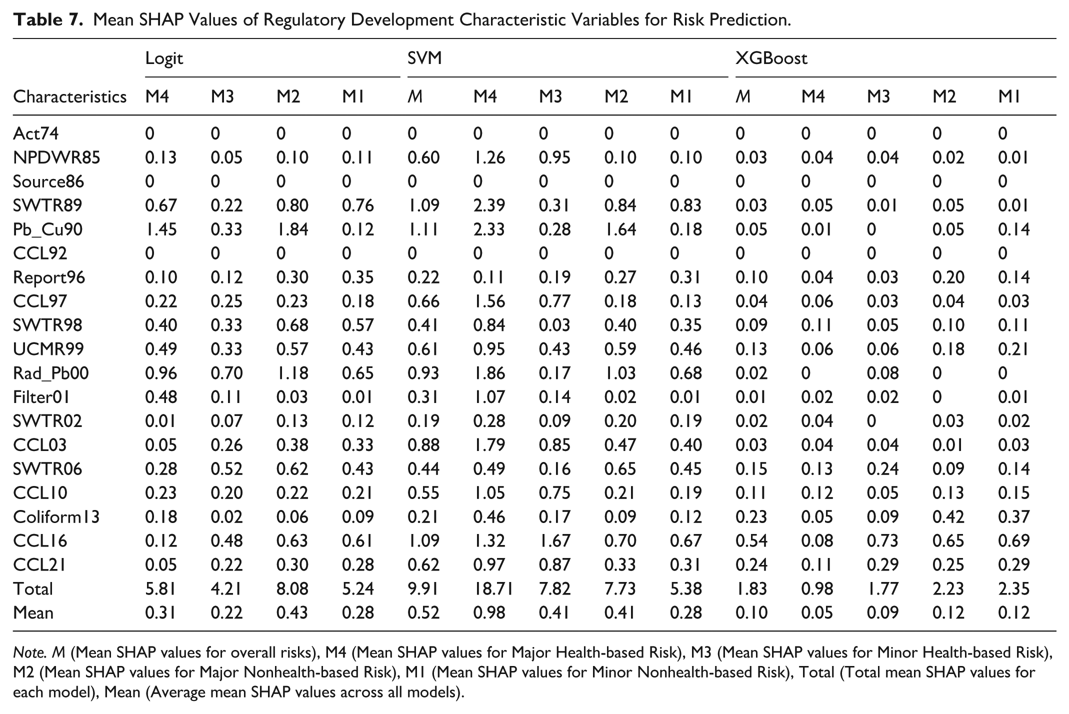
Note. M (Mean SHAP values for overall risks), M4 (Mean SHAP values for Major Health-based Risk), M3 (Mean SHAP values for Minor Health-based Risk), M2 (Mean SHAP values for Major Nonhealth-based Risk), M1 (Mean SHAP values for Minor Nonhealth-based Risk), Total (Total mean SHAP values for each model), Mean (Average mean SHAP values across all models).

Moreover, SWTR89, Pb_Cu90, and SWTR98 exhibit higher Sohol ST values (0.05-0.2) for Major risks (H) and Major risks (N) in the Logit and SVM models (see Appendix 5). In the XGBoost model, Pb_Cu90, CCL92, SWTR06, CCL10, CCL16, and CCL21 show elevated Sohol S1 and ST values (0.08-0.55) for Major and Minor risks (H) and overall risk predictions. CCL92, SWTR98, UCMR99, CCL10, and CCL16, and CCL21 have higher Sohol ST and S1 values (0.05-0.2) for Major and Minor risks (N).

Additionally, Sobol S2 analysis revealed notable differences in interaction patterns across risk categories. For overall risks (Appendix 6), High School exhibited the strongest positive pairwise interaction effects with most other variables, indicating that low educational attainment can substantially amplify risk when combined with other factors. For Major risks (N; Appendix 9), Asian%, Native%, and High School consistently showed positive interactions with multiple variables, suggesting these characteristics play a significant role in compounding vulnerabilities. Similarly, for Minor risks (N; Appendix 10), Bachelor, Black%, and High School demonstrated persistent positive interaction effects across several variable pairs. In contrast, analyses for Major and Minor risks (H; Appendices 7 and 8) revealed generally low interaction effects, indicating that these risks are primarily driven by independent contributions of individual variables rather than synergistic interactions.

Discussion

The XGBoost Model Exhibits Better Prediction Performance

The XGBoost model predicts a higher proportion of actual positive risks and a lower proportion of incorrect predictions compared to the Logit and SVM models (see Table 4). This superior performance is attributed to XGBoost’s tree-based structure and gradient boosting mechanism, which iteratively enhances its ability to capture complex, nonlinear relationships among features (variables), handle feature interactions, automatically select the most important variables, and improve predictions for underrepresented Major and Minor risks (H). These capabilities make XGBoost particularly suited for predicting PWS risks influenced by multifaceted, multilevel, longitudinal, and nonlinear factors. For example, the 2014 Flint drinking water crisis in Michigan was shaped by numerous factors, including historical industrial pollution, outdated infrastructure, economic downturns, poverty, racism, political struggles, and delayed responses.^23,24,33,34

In contrast, the Logit model assumes a linear relationship between risks and independent variables, limiting its ability to analyze complex datasets with continuous, categorical, and binary variables. This restricts its capacity to simulate the nonlinear relationships contributing to PWS risks. Similarly, the SVM model struggles to find an optimal hyperplane for predicting risks from large datasets with complex and imbalanced structures.

The XGBoost Model is Suboptimal for Predicting Major and Minor Risks (H)

The lower Precision, Recall, F1 Score, and AUC-ROC values, combined with high Accuracy for Major and Minor health-based risks (H), indicate that the XGBoost model predicts a smaller portion of actual positive health-based risks compared to its performance on nonhealth-based risks (see Table 4). Specifically, the low Recall values for health-based risks in Table 4 indicate a higher likelihood of Type II errors. This highlights the need for strategies that prioritize reducing false negatives in future research.

This suboptimal performance is likely due to the significantly larger number of nonhealth-based risks relative to health-based risks (see Figure 2 and Table 1), leading to fewer data points available to train the model on predicting health-based risks. Additionally, identifying Major and Minor health-based risks (H) may require more independent variables related to political bargaining and decision-making following complex water parameter testing, whereas defining nonhealth-based risks (N) primarily involves assessing document submissions.

Moreover, incorporating Type I/II error rates, Precision–Recall (PR) curves, and class-weighted F1 scores can provide a more comprehensive understanding of the model’s limitations and inform future improvements, even though these measures will not change the conclusion that XGBoost is suboptimal for predicting health-based risks. PR curves reveal performance across thresholds and underscore the challenge of identifying positive cases, while class-weighted F1 scores may slightly enhance reported performance for minority classes (health-based risks).

Community and Regulatory Characteristics Influence Risks More Than PWS Characteristics

In the XGBoost model, the mean SHAP values for PWS characteristic variables are 0.03 and 0.04 (see Table 5), which are notably lower than the values for community characteristic variables (0.09-0.20, see Table 6) and regulatory development variables (0.05-0.12, see Table 7). Similar trends are observed in the Logit and SVM models. Additionally, the Sobol S1 and ST indices for community characteristics (see Appendix 4) are consistently higher than those for PWS and legal development characteristics (see Appendices 3 and 5) across the 3 models, indicating that community factors contribute more to overall output variance than system-level or regulatory variables.

These findings suggest that community and regulatory development characteristics have a greater influence on risk predictions than PWS characteristics, consistent with previous studies indicating that these factors are fundamental social determinants of drinking water quality.^{15 -17} They partially contribute to risks through pathways such as PWS investment and management, environmental enforcement, and public education.^20,23,25 New regulations may further amplify this influence by defining more types of risks, tightening thresholds for environmental violations, or mandating additional PWS improvements.

Importantly, these findings do not imply that community or regulatory efforts should replace investments in PWS infrastructure and management, nor that social determinants should outweigh water quality and hydrological factors in ensuring safe drinking water. Rather, the results indicate that social context carries greater predictive weight for long-term PWS risks, while water science and engineering remain essential for managing the risks.

Mean SHAP values for overall and major health-based risks in the XGBoost model in Table 6 suggest several macro-policy implications. First, reducing community poverty and improving educational attainment can enhance local capacity to mitigate PWS risks over time. Second, higher education levels and prioritization by state and county-level leadership may increase awareness and responsiveness to these risks. In this context, a public drinking water surveillance system – supported by well-educated individuals and engaged local leaders – may increase such awareness and responsiveness. Moreover, greater policy attention is warranted for communities with high concentrations of minority populations and elevated levels of industrial activity, as these areas are projected to face higher PWS risks in the long term. Additionally, Table 6 and the distribution of health-based PWS violations in Table 1 indicate that regulatory compliance efforts should prioritize contaminants including coliform bacteria, arsenic, nitrate, and disinfection byproducts, particularly in systems serving communities with higher poverty rates, lower educational attainment, greater proportions of Asian residents, and elevated industrial activity.

Also, Sobol S2 analysis shows that High School, Asian%, Native%, and Black% consistently exhibit strong interaction effects with other variables, amplifying Major and Minor risks (N). These findings underscore the need for culturally tailored risk communication, education programs, and infrastructure investments in communities with lower educational attainment and areas with higher minority populations. In contrast, Major and Minor risks (H) are largely driven by individual variables, suggesting that interventions in these domains can focus on single determinants rather than complex multi-factor strategies.

Moreover, Republican governorship and county-level support for Republican presidential candidates are associated with slightly higher levels of PWS risks compared to Democratic governorship and county-level support for Democratic presidential candidates (see Table 6). Notably, the mean SHAP values do not imply causation; rather, the findings suggest potential weak associations between Republican governorship, voter preferences for Republication candidate, and PWS risks in Michigan. These weak associations may be attributed either to Republican leaders’ prioritization of fiscal concerns over public health^{35 -41} or to other covariates. For instance, Republican voters are more likely to reside in suburban and rural communities, which often rely on smaller PWS and consequently face higher levels of drinking water risks.

Similarly, private ownership is associated with slightly higher levels of PWS risks compared to federal, state, and local governmental ownership (see Table 5, particularly the XGBoost model results). The mean SHAP values similarly suggest an association, rather than causation, between private ownership and elevated risk levels after accounting for other variables. However, these associations may be biased due to the significantly larger number of data points for privately owned PWS compared to other ownership types and the reliance on environmental data from EPA law enforcement, which may enforce stricter regulations on private PWS than on government-owned ones. Future research could conduct difference-in-differences analyses to investigate potential causal relationships between partisan associations and PWS risks.

XGBoost Performs Comparably to the Water Parameter-Based Prediction Approach

The performance of the XGBoost model is comparable to water parameter-based prediction approaches. Nine out of 12 prior studies used ANN models to predict drinking water quality, contamination events, or leakages, reporting accuracy values between 52% and 99%, Concordance Index values from 0.7 to 0.9 (with 1 indicating perfect predictions), R² values between 0.35 and 0.93, and RMSE or other error values ranging from 0.00004 to 159 (with lower values indicating higher accuracy; see Appendix 2). Precision (0.99) and Recall (0.55) were reported in only one study. Our XGBoost model, using PWS, community, and regulatory development characteristics, achieved accuracy values of 0.8 to 0.99, although Precision (0.59-0.87) and Recall (0.21-0.73) were lower. These characteristics are fundamental social determinants of risk. The model was trained using 57 independent variables and over 63 000 data points, significantly exceeding the number of water quality and hydrological parameters used in prior studies. Additionally, the XGBoost model is cost-effective and suitable for long-term forecasting, as it utilizes data from EPA and census datasets, eliminating the need for costly sensors and laboratory equipment. ⁴²

Limitations and Future Research

First, future research may apply our models or approach to predict unregulated contaminants based on PWS, community, and other social characteristics, as this study predicts regulated contaminants. Unregulated contaminants such as Per- and Polyfluoroalkyl Substances (PFAS), Pharmaceuticals and Personal Care Products (PPCPs), and Hormones and Endocrine Disruptors may pose potential public health risks, with social factors influencing exposure. ⁴⁵ While the U.S. EPA is studying their presence and prevalence in PWS, enforceable MCL have not yet been established. Current water parameter-based studies also have not focused on predicting these contaminants (see Appendix 2).

Second, future research may incorporate more data points and additional decision-making variables to improve the Precision of predicting Major and Minor risks (H). Third, future research may use time series data to predict the timing of PWS risks, as this study predicts probabilities from cross-sectional data.

Fourth, future research could enhance the XGBoost model by incorporating additional features, advanced techniques (eg, feature engineering, hyperparameter optimization), or strategies such as weighted loss and ensembling with other machine learning models to improve prediction performance or address specific risks in particular contexts. We did not implement these enhancements due to their marginal performance gains compared to the significant increase in interpretation complexity and computational costs. Additionally, compared to linear or logistic regression models, XGBoost and SVM models often require more computing resources and a trial-and-error approach to optimize model architecture and learning parameters.

Fifth, data quality is a concern as the Michigan government is correcting some inaccurate facility monitoring reports, ⁴⁶ which affects prediction performance for Major and Minor risks (N). The performance is also limited by approximating PWS service population characteristics using the best-fitting boundary census data.

Sixth, future research could examine the relationship between individual health outcomes – particularly waterborne diseases – and drinking water quality, with attention to how socio-economic and socio-demographic factors (eg, bottled water industry) mediate this relationship. This study introduces a new methodological approach (an overall “how-to”) for predicting drinking water quality using PWS characteristics and social determinants of health (non-medical factors). Importantly, our approach focuses on predicting the service quality of PWS at the plant level (point of entry), rather than individual health outcomes at the household level (point of use).

Future research could examine the generalizability of this predictive approach across other U.S. states and potentially international contexts. Although this study focuses on Michigan, the state comprises approximately 1/15th of all U.S. PWS and reflects governance structures and socio-economic characteristics that are broadly representative of many states.

Conclusion

We compared the Logit, SVM, and XGBoost models for predicting risks using PWS, service community, and regulatory development characteristics, rather than water quality and hydrological parameters. Our findings show that: (1) the XGBoost model outperforms the Logit and SVM models due to its ability to capture complex, nonlinear social relationships underlying the risks; (2) XGBoost is less effective at predicting Major and Minor health-based risks (H) compared to other risk types; (3) community and regulatory characteristics have a greater influence on risk prediction than PWS characteristics; and (4) XGBoost’s performance is comparable to water parameter-based approaches, with the added benefits of lower cost and suitability for long-term forecasting.

Our study presents a foundational yet practical approach for predicting PWS risks using readily available system, socio-economic, and regulatory data. This new approach offers significant potential for residents and environmental advocates to anticipate and prepare for long-term risks. Policymakers can use these insights to proactively address water safety challenges by enacting more effective policies, allocating resources strategically, and empowering communities. This highlights the critical need for policies that address underlying social determinants to mitigate risks, emphasizing the role of regulatory frameworks, economic development, and social justice in ensuring water safety. Furthermore, our study encourages future scholars to apply computational and machine learning methods, which surpass linear regression, to better understand and address complex water-society interactions.