Sage Journals: Discover world-class research

Abstract

Chinese

Neighbourhood socioeconomic disadvantage has a profound impact on individuals’ earnings and life satisfaction. Since definitions of the neighbourhood and research designs vary greatly across studies, it is difficult to ascertain which neighbourhoods and outcomes matter the most. By conducting parallel analyses of the impact of neighbourhood deprivation on life satisfaction and earnings at multiple scales, we provide a direct empirical test of which scale matters the most and whether the effects vary between outcomes. Our identification strategy combines rich longitudinal information on individual characteristics, family background and initial job conditions for England and Wales with econometric estimators that address residential sorting bias, and we compare results for individuals living in choice-restricted social housing with results for those living in self-selected privately rented housing. We find that the effect of neighbourhood deprivation on life satisfaction and wages is negative for both outcomes and largely explained by strong residential sorting on both individual and neighbourhood characteristics rather than a genuine causal effect. We also find that the results overall do not vary by neighbourhood scale.

Keywords

demographics employment/labour life satisfaction longitudinal analysis neighbourhood poverty/exclusion

Introduction

The extent to which neighbourhood socioeconomic deprivation impacts on individual wellbeing, a phenomenon commonly known as ‘neighbourhood effects’, has been the focus of much scholarly debate and empirical research in the social sciences. While it is widely acknowledged that where people live can have a profound impact on their wellbeing, quantifying the importance of neighbourhood effects is very challenging because of the complex processes of residential self-selection and neighbourhood-specific correlated effects (see e.g. Duncan et al., 1997; Durlauf, 2004; Manski, 1995; Sampson et al., 2002). There also is the challenge of identifying the spatial scale(s) over which the specific neighbourhood effect under investigation may operate (Galster, 2008; van Ham and Manley, 2012). Neighbourhood definitions abound in the empirical literature; however, the choice of unit used is often not informed by theoretical considerations (Dietz, 2002: 541) but instead dictated by ‘convenience and pragmatism’ (van Ham and Manley, 2012: 2791); localities are lifted ‘off the shelf’ and may lack the characteristics through which neighbourhoods may affect individual outcomes: the bonds between people and places created by time and events, which influence the social organisation and architectural design of the local community.

There have been promising developments in how research can better operationalise the ‘neighbourhood’ in neighbourhood effects research, even using ‘off the shelf’ units. The first development is the use of ‘bespoke’ neighbourhoods. These define a neighbourhood area based on the distance from a specific point, or as the number of people situated nearest to a specific location (e.g. home postcode). Compared with using standard administrative geographies, such ‘bespoke’ neighbourhood characteristics are regarded as capturing better the environment surrounding each individual and, by placing the individual at the centre of the neighbourhood, the risk of biased estimates resulting from boundary effects is reduced (Hedman et al., 2015: 200). The second development is the more meaningful delineation of official spatial reporting units at immediate scales. In Britain, new boundaries were delineated for the 2001 population census based on spatial proximity, natural boundaries as well as homogeneity of dwelling type and tenure so that aggregations to areas of around 600 households (~1500 people, so-called Lower Super Output Areas, LSOAs) would refer to localities that local people conceive as neighbourhoods. LSOAs are ‘substantially smaller and more internally homogenous than the area geographies that have been relied upon by many previous studies, enhancing our ability to uncover evidence of neighbourhood processes operating within local communities’ (Sutherland et al., 2013: 1055–1056).

Much British neighbourhood research since 2001 has relied on neighbourhood characteristics at the LSOA level (see e.g. Platt et al., in press). It remains an empirical question, however, whether these units are the most appropriate scales for measuring all types of neighbourhood effects. With over a dozen distinct effect mechanisms identified, ranging from social interactive to environmental, geographical and institutional mechanisms (Galster, 2012), it would seem reasonable to expect many different scales to be important for individual wellbeing: neighbourhoods, because of variations in peer groups, social organisations and social networks; political jurisdictions, because of variations in health, education, recreation and safety programmes; and metropolitan areas, because of providing locations of employment of various types and skill requirements (Galster, 2005). We may expect social interaction effects to operate at smaller scales than the 1500 people in the LSOA, for example, since ‘150 to 250 people can maintain [the] close, personal interaction’ and ‘400 to 600 can maintain [the] more casual form[s] of interaction’ (Talen, 2019: 17) which underpin effects based on (possible) interacting with others. By contrast, when examining institutional effects that may manifest through local council policies or geographical effects such as labour market competition, neighbourhoods defined at broader spatial scales may be more relevant (Andersson and Musterd, 2010: 27; Petrovic et al., 2019).

The most direct approach to test empirically ‘which scale matters’ is to conduct parallel analyses of a particular outcome using neighbourhood indicators measured at different scales. Ideally, such an approach considers multiple outcomes where the effect of the neighbourhood may be expected to transpire at different scales. This is the approach we will adopt here, focusing on the effect of neighbourhood deprivation on earnings and life satisfaction. We draw on rich individual-level panel data for England and Wales linked with information from census records for 2001 and 2011. We have longitudinally harmonised the census data for output areas in 2001 and defined neighbourhood deprivation at multiple bespoke scales. The approach combines the advantages of well-defined neighbourhood units at very small scales with that of using egocentric neighbourhoods. Moreover, we address key identification challenges by using a wealth of background information from the longitudinal survey, including individuals’ residential location at different points in time, and explore how much of the effect of neighbourhood deprivation is due to unobserved characteristics of both individuals and neighbourhoods. We find that people who live in more deprived areas are less satisfied with their lives and that they have lower earnings; however, the negative association between neighbourhood deprivation and wellbeing is largely due to non-random selection into neighbourhoods and not a genuine causal effect. We also do not find evidence for variation in the size of the neighbourhood effect across spatial scales.

Neighbourhood effects: Identification challenges and empirical findings

Identification challenges

The neighbourhood effects literature is vast and has been widely reviewed across disciplines (e.g. Dietz, 2002; Diez Roux and Mair, 2010; Durlauf, 2004; Friedrichs et al., 2003; Galster, 2008; Sampson et al., 2002; van Ham and Manley, 2012). We contribute to existing reviews with a focus on how the empirical research has defined neighbourhoods, how effects vary by neighbourhood scale and how the research accounted for the various sources of unobserved differences between both individuals and neighbourhoods, including non-random selection into neighbourhoods. Methods to address residential selection bias include restricting the sample to individuals for whom residential location is exogenous (e.g. Dujardin et al., 2009; O’Regan and Quigley, 1996), exploiting information from quasi-random housing assignment programmes (e.g. Chetty et al., 2016), or implementing fixed effects (e.g. Knies, 2012), propensity score (Brännström, 2004) or instrumental variables estimators (e.g. Dujardin and Goffette-Nagot, 2010). A small number of studies have modelled residential mobility directly by combining the estimation of a discrete choice model of neighbourhood selection with the posterior estimation of the neighbourhood effect model (Hedman et al., 2011; van Ham et al., 2018). Comparing results across estimation strategies suggests that studies that ignore individual self-selection into neighbourhoods tend to find sizeable neighbourhood ‘effects’, while those implementing some correction for selection bias or using experimental designs do not. Findings of neighbourhood effects, therefore, need to be discussed regarding how rigorously residential selection bias has been addressed.

Reviews of the empirical and theoretical literature provide little guidance on which neighbourhood effect operates at which scale and empirical studies have looked for each type of neighbourhood effect at ‘very small’ (<500 people) to ‘very large’ (>100,000 people) neighbourhood scales (Knies et al., 2020). A number of British studies compared the importance and intensity of neighbourhood effects at bespoke neighbourhood scales ranging from the nearest 500 to 10,000 people.¹ Buck (2001), using enumeration areas from the 1991 census as building blocks, found a negative impact of neighbourhood deprivation on a range of socioeconomic outcomes at all scales but with diminishing intensity as the neighbourhood boundaries expanded. Residential selection bias was not considered. Similar bespoke neighbourhood data have been linked to British surveys to examine income transitions (Bolster et al., 2007), voting patterns (Johnston et al., 2004) and mental health (Propper et al., 2005), providing further empirical evidence on the importance of the socioeconomic and demographic composition of the neighbourhood for individual behaviour and wellbeing, particularly at the most immediate neighbourhood scales. Our study, too, will adopt this approach.

Neighbourhood effects on life satisfaction

To our knowledge, no study has investigated how neighbourhood deprivation affects life satisfaction in Britain. A number of studies based on individual panel data for other countries have examined the effect of related markers of neighbourhood socioeconomic status on life satisfaction and tested for social interactive neighbourhood effect mechanisms. Knies et al. (2008), defining neighbourhoods as postcode areas with an average population of ~9000 people in Germany, found sizeable negative effects of living amongst more affluent neighbours in cross-sectional models but not in models that controlled for individual-level unobserved heterogeneity. When defining neighbourhoods at the much more immediate scale of street-sections (~25 households on average), the negative effect was robust in models that controlled for unobserved individual heterogeneity, and in models that additionally focused on non-movers (i.e. absorbing neighbourhood fixed effects), see Knies (2012). Dittmann and Goebel (2010) operationalised neighbourhoods in Germany as blocks of houses with an average of 8 to 25 households. Their analysis found that people are more satisfied with their lives when their own social status is higher than their neighbours’ status and vice versa. The findings were largely robust to the addition of individual fixed effects, albeit somewhat smaller. Similar effects of neighbourhood social rank on satisfaction with one’s earnings were found for small neighbourhoods comprising 150–600 households in Denmark (Clark et al., 2009). Shields et al. (2009) studied the relationship between life satisfaction and several markers of neighbourhood socioeconomic deprivation using Australian panel data, operationalising neighbourhoods as census areas comprising ~250 households. The analysis showed that some factors associated with greater neighbourhood disadvantage (i.e. living in a neighbourhood with higher concentrations of immigrants and of single parents) were negatively associated with life satisfaction, while other measures (i.e. unemployment, homeownership, proportion professional workers and proportion older population) were not.

We may conclude from these studies that neighbourhood disadvantage does affect life satisfaction but the direction of the effect may be scale-dependent: in the most tightly drawn neighbourhoods affluence rather than deprivation may hurt (despite richer neighbourhoods offering, in all likelihood, higher-quality amenities).

Neighbourhood effects on earnings

A number of studies have used a multiscale approach to test for differences in the size of the neighbourhood effect on individual earnings, predominantly using Swedish register data. Andersson and Musterd (2010) found that the effects of neighbourhood socioeconomic disadvantage were most pronounced at the scale of 400–600 people (i.e. Small Area for Market Statistics, SAMS) and statistically not significant at the larger municipality level. In areas targeted by local regeneration policies, characteristics at the block level (i.e. ~40–60 households) were most important. In related studies, the authors showed that the proportion of low-income males in the SAMS, too, reduces labour-income, and this was robust to absorbing time-invariant unobserved individual characteristics and to restricting the analysis to non-movers (Galster et al., 2008); Galster et al. (2015) went on to show that the effect of low-income neighbours is non-linear, increasing sharply when the proportion of low-income neighbours exceeds 40%. The importance of neighbourhood effects on earnings appears quite small, however. Brännström (2005) found that the level of neighbourhood income during childhood at the scale of census tracts and parishes explained only ~1% of the variance in individual earnings, while childhood income at slightly smaller scales explained none of the variance in earnings during adulthood (Lindahl, 2011). Neighbourhood effects may also work in opposite directions at different scales. Mellander et al. (2017) found that the effect of higher-skilled neighbours was positive and sizeable for the block and SAMS scales, and negative and minute for the municipality and local labour market scales.

Compared with the richness of Swedish studies, empirical evidence for Britain is scant. Bolster et al. (2007) examined the association between neighbourhood disadvantage and income growth drawing on bespoke neighbourhood data linked to panel data from the British Household Panel Survey (BHPS) for Britain for the period 1991–2000. The study adopted a fixed effects modelling framework and found no neighbourhood effects on income growth over one, five and ten years, nor much scale-dependency. For property owners and couples, however, there was a small and positive effect of neighbourhood disadvantage on subsequent income growth, and this was most marked when neighbourhoods were defined as bespoke areas with a minimum population size of 500. For owners, neighbourhood selection may be particularly marked, and the fixed effects approach does not remove bias associated with residential sorting on time-variant unobserved characteristics of individuals (e.g. Hedman et al., 2015). However, Propper et al. (2007) found that neighbourhood disadvantage at the 500-neighbours scale also significantly reduced the income in the following years of social renters, who have a very limited residential choice.

In sum, the empirical literature is somewhat inconclusive about the scale and direction of the effect of neighbourhood disadvantage on life satisfaction and earnings, but the effect size generally is reduced or wiped out once non-random selection into neighbourhoods is accounted for. By conducting parallel analyses of the impact of neighbourhood deprivation on life satisfaction and earnings, we provide a direct empirical test of which scale matters the most, and whether effects vary, for these two outcomes.

Empirical strategy

Modelling framework

We employ regression models to estimate the effect of neighbourhood deprivation on life satisfaction and earnings. The analysis proceeds in four stages. To set the scene, we estimate wellbeing models – one for each bespoke neighbourhood scale – which account for individual heterogeneity in basic demographic and socioeconomic characteristics but do not attempt to address the main identification challenges discussed earlier. In the second through fourth stages, we apply methods that help address the identification issues to get an unbiased and consistent estimate of the effect of neighbourhood deprivation on individual wellbeing. The remainder of this section describes these stages.

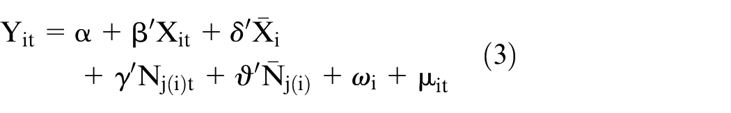
We start by adopting a standard model that assumes that exogenous individual and neighbourhood characteristics have a direct impact on the level of wellbeing:

Y_{it} = α + β' X_{it} + γ' N_{j (i) t} + ε_{it}

(1)

where i denotes individuals, j neighbourhoods and $t$ > time. Individual wellbeing $(Y_{it})$ > is a function of individual characteristics ( $X_{it}$ > ) and neighbourhood characteristics $(N_{j (i) t}$ > ) that have been shown to influence wellbeing, and the error ( $ε_{it}$ > ). This model is implemented using the pooled ordinary least squares (OLS) estimator. As we are working with panel data, all standard errors are adjusted for clustering on individuals and for heteroscedasticity.

In the first stage, we include a standard set of individual demographic and socioeconomic characteristics and area characteristics that may otherwise confound the association between neighbourhood deprivation and wellbeing. For instance, ethnicity is a robust predictor of life satisfaction and earnings (Brynin and Güveli, 2012), and macro trends in labour markets affect both wellbeing outcomes as well as area levels of deprivation.

Next, we gauge the importance of neighbourhood selection on a set of observable characteristics relating to family background. As parents play a major role in helping their children to set up homes of their own, we include measures of parental socioeconomic status (i.e. the higher of the mother’s or father’s social class when the respondent was aged 14) and of their own socioeconomic status when entering the labour market (i.e. the social class of the first job after leaving full-time education). The conjecture is that these factors, dubbed here as ‘initial conditions’, will impact the initial neighbourhood choice and that the effects of previous choices will linger to impact on the current level of wellbeing (Hedman et al., 2015; Sharkey and Elwert, 2011).

Nevertheless, there may be other unobserved individual characteristics (e.g. residential preferences) and neighbourhood conditions correlated with area deprivation, leading to inconsistent estimates of the effect of neighbourhood deprivation on wellbeing. Furthermore, in the case of individual earnings, there may be simultaneity bias because individuals and households with lower earnings generally cannot afford to live in the most sought-after neighbourhoods and hence may have to live in more deprived areas.

An advantage of the panel nature of our data set is that it allows us to separate individual unobserved factors that are time-invariant from those that are not. Equation (1) may be extended to

Y_{it} = α + β' X_{it} + γ' N_{j (i) t} + ω_{i} + μ_{it}

(2)

where $ω_{i}$ > captures individual-specific time-invariant features. In the economics literature, the fixed effects approach is typically operationalised using the within panel estimator, but the correlated random effects estimator shares the advantages of the fixed effects approach, as shown by Mundlak (1978), is more efficient than the fixed effects estimator and allows us to examine the effects of time-invariant characteristics (Bell et al., 2019).² Thus, we implement the models using the random effects estimator and apply the Mundlak correction:

\begin{matrix} Y_{it} = α + β' X_{it} + δ' {\bar{X}}_{i} \\ + γ' N_{j (i) t} + ϑ' {\bar{N}}_{j (i)} + ω_{i} + μ_{it} \end{matrix}

(3)

All models are estimated using the xtreg command in Stata 15. Next, just as individual fixed effects allow us to take into account spatial sorting on time-invariant unobserved features, there may be unobserved aspects of neighbourhoods that not only make them (un)attractive places to live but which may also be correlated with neighbourhood deprivation. To account for neighbourhood-specific features, we add the component $ρ_{j}$ > to Equation (2) and estimate the following two-way fixed effects model:

Y_{it} = α + β' X_{it} + γ' N_{j (i) t} + ω_{i} + ρ_{j} + μ_{it}

(4)

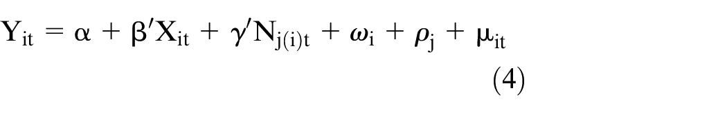
We use the procedure developed by Correia (2017) to deal with the large number of fixed effects able to be estimated in our data. This approach allows us to show how much the effect of neighbourhood deprivation may be biased because of correlated unobserved neighbourhood characteristics but precludes reporting of time-invariant characteristics.

Robustness tests

To test the sensitivity of our results to omitted sources of selection bias unaccounted for in our models, we apply a set of sample restrictions and repeat the same model specifications and statistical estimators. We contrast the estimation results for individuals living in social housing against results for those living in private rented accommodation. We argue, as others have before us (Propper et al., 2007; Weinhardt, 2014), that residential location is essentially exogenous for social renters in England and Wales. Although local authorities tend to have some form of choice-based allocation schemes with general priority rules, because of the shortage of social housing social renters have a very limited choice in selecting neighbourhoods or moving from the initial residential allocation. In contrast, for private renters, the residential choice is likely to be endogenous as they can and do move around more freely and across a greater range of different neighbourhoods. Consequently, we will consider social renters as ‘less selected’ and private renters as ‘more selected’ and would expect the associated biases to be attenuated in these samples. Moreover, and despite social housing allocation not being fully random, we would not expect marked differences between the pooled OLS and the fixed effects estimates for social renters because unobserved individual factors should not have played a role in determining the housing allocation.³

Data

Individual wellbeing outcomes and control variables

We use individual-level panel data from the first six waves of Understanding Society (University of Essex et al., 2018). The panel study started in 2009 with a nationally representative, stratified, clustered sample of around 30,000 households in the UK and was enhanced further in the second and sixth waves when the continuing sample, around 8000 households-strong, of the BHPS and a new immigrant and ethnic minority boost (IEMB), respectively, were added. The annual face-to-face survey collects information about various aspects of people’s lives, including education, employment, income and health. All members of the household aged 16 and above are eligible for an interview. Overall, 76,151 individuals provided a full interview in the first six rounds of annual interviews, offering 292,322 person-year observations.

Our outcome variables of interest are life satisfaction – a reflective appraisal of how well life is going and has been going (Argyle, 1999), and hourly wage. The life satisfaction measure is the response to the question ‘How satisfied are you with life overall?’ with responses ranging from 1 ‘completely dissatisfied’ to 7 ‘completely satisfied’. The hourly wage measure is derived from the ratio between usual gross monthly salaries (including any overtime compensation, bonuses, commission, tips and tax refund before any deduction) and hours normally worked and overtime for individuals in paid employment (excluding self-employment).

All models include basic socioeconomic and demographic controls that have been linked to the two wellbeing outcomes, namely: age, gender, ethnicity, whether the respondent was born in the UK, marital status, presence of children in the household, highest educational qualification, social class and the current main economic activity status. In the life satisfaction models only, we additionally include net equivalent household income.

Bespoke neighbourhoods and spatial controls

We used the postcode of survey members’ addresses to link to geocoded information at the output area level from the Census 2001 and 2011 for England and Wales to define the bespoke geographies employed in the research. We addressed, inasmuch as is feasible, changes in output area boundaries across the two censuses (see Technical Appendix, available online) and created bespoke neighbourhoods by aggregating the longitudinally harmonised output areas (OAs) 2001 and 2011 (henceforward: OA) closest to the respondents’ residential postcode until the pre-defined population threshold (i.e. the nearest n population, where n = 500, 1000 … 10,000 in intervals of 1000) was reached. Whilst this follows the standard procedure for creating bespoke areas, we preserved the nested structure of census areas by restricting the nearest OA to those from the same LSOA in the first instance. Once exhausted, we picked from the nearest OA in a different LSOA in the same Middle Layer Super Output Area (MSOA); then moving to a different MSOA in the same local authority, and so on until the predefined population thresholds were crossed.⁴

Our key measure of interest is neighbourhood deprivation. Following precedents in the empirical literature, and to allow us to relate our findings more closely to Buck’s (2001) foundational work on neighbourhood effects for multiple outcomes and at multiple scales, we use the Townsend Deprivation Index (Townsend et al., 1988). The index summarises four census indicators at the neighbourhood scale: (1) proportion of economically active residents who are unemployed (logged), (2) proportion of residential households who do not own a car or van, (3) proportion of households not in owner-occupied accommodation, and (4) proportion in overcrowded households (logged).⁵ We used the aggregated values for all OAs involved in the respective bespoke neighbourhood in 2001 and 2011 to forecast the neighbourhood characteristics in the study period (using compound annual growth rates).⁶ The components are standardised and then summed. To provide a more realistic depiction of the local context of a given neighbourhood, we standardised the index using the local authority mean and standard deviation in deprivation. Higher values indicate greater relative deprivation and a value of zero represents the average level of deprivation in the local authority area.

Models additionally take into account conditions at higher spatial scales that may influence individual wellbeing and may be confounded with neighbourhood deprivation: whether the respondent lives in England or Wales, the national and local unemployment rate and an area classification.

Linkage of the panel data with geographically coded data necessitated the sample to be restricted to respondents with a valid postcode who live in England and Wales. The IEMB sample was dropped for lacking longitudinal information. We also restricted the analysis to those aged 16–74 years and removed observations whose hourly wages fell short of the age- and year-specific national minimum wage (which ranged from £3.30 to £7.20 in the period studied), or whose wages were 25% higher than the 99th percentile. Otherwise, all cases with complete information are included in the analysis. The subsample with wages is somewhat younger, slightly more educated and lives in slightly less relatively deprived neighbourhoods than the general population considered in the life satisfaction models (see Supplemental Material A2, available online).

Results

Full sample results

Table 1 reports the results of the pooled OLS regressions of life satisfaction and hourly wage on individual demographic, socioeconomic and area structural characteristics. Neighbourhood deprivation is measured at the smallest scale (i.e. the longitudinally harmonised output areas, OA).

Table 1.

Pooled OLS regression of life satisfaction and hourly wage on neighbourhood deprivation at the output area scale.

	Life satisfaction		Hourly wage (log)
	b-coef.	T-stat	b-coef.	T-stat
Individual socio-demographics
Age	−0.09	−30.55***	0.04	29.99***
Age squared	0.00	29.14***	−0.00	−25.43***
Female	0.07	6.15***	−0.18	−35.37***
Ethnicity (ref. White British)
Caribbean/African Black	−0.15	−3.93***	−0.02	−1.41
Asian	−0.18	−6.35***	−0.08	−6.31***
Other	−0.14	−4.84***	0.02	1.49
Born in UK	−0.05	−2.07*	0.04	3.84***
Marital status (ref. single)
Married/cohabiting	0.30	15.40***	0.05	6.95***
Divorced/separated	−0.10	−3.39***	0.02	1.62
Widowed	0.02	0.52	0.07	2.52*
Educational qualification (ref. degree)
Other higher degree	−0.06	−2.87**	−0.15	−18.12***
A-level, etc.	−0.09	−5.09***	−0.19	−24.69***
GCSE, etc.	−0.11	−6.16***	−0.26	−31.85***
Other or no qualification	−0.12	−5.91***	−0.32	−32.69***
Own social class (ref. managerial/professional)
Intermediate	−0.06	−3.55***	−0.26	−37.16***
Routine	−0.06	−3.55***	−0.38	−57.22***
No paid job	−0.23	−7.20***
Economic status (ref. employed)
Unemployed	−0.35	−9.26***
Retired	0.37	10.65***
Other^a	−0.15	−4.87***
Household income (log)^b	0.17	14.00***
Child(ren) in household	0.06	4.64***	0.02	3.37***
Long-term illness	−0.48	−40.01***	−0.03	−6.87***
Spatial measures
Neighbourhood deprivation	−0.07	−10.84***	−0.05	−17.72***
Spatial control variables
Lives in England and Wales (ref. England)	−0.03	−1.23	−0.03	−3.05**
National unemployment rate	0.02	2.95**	−0.03	−16.61***
Local unemployment rate	−0.01	−2.94**	−0.01	−12.17***
Area classification (ref. inner London)
Outer London	−0.03	−0.82	−0.04	−2.60**
West Midlands	−0.04	−0.95	−0.15	−8.79***
Greater Manchester	0.07	1.67	−0.18	−10.67***
West Yorkshire	0.09	2.08*	−0.21	−10.36***
Liverpool	0.10	1.49	−0.20	−7.76***
Tyneside	0.09	1.68	−0.19	−9.08***
South Yorkshire	0.00	0.08	−0.23	−10.02***
Urban over 250k	0.02	0.62	−0.19	−13.35***
Urban over 100k to 250k	0.06	1.86	−0.19	−13.49***
Urban over 50k to 100k	0.05	1.37	−0.19	−12.57***
Urban over 10k to 50k	0.08	2.46*	−0.19	−13.26***
Urban over 3k to 10k	0.11	2.95**	−0.21	−12.12***
Rural	0.08	2.37*	−0.19	−13.35***
Constant	5.69	45.07***	2.43	73.63***
Observations	129,988		64,963
R-squared	0.097		0.450

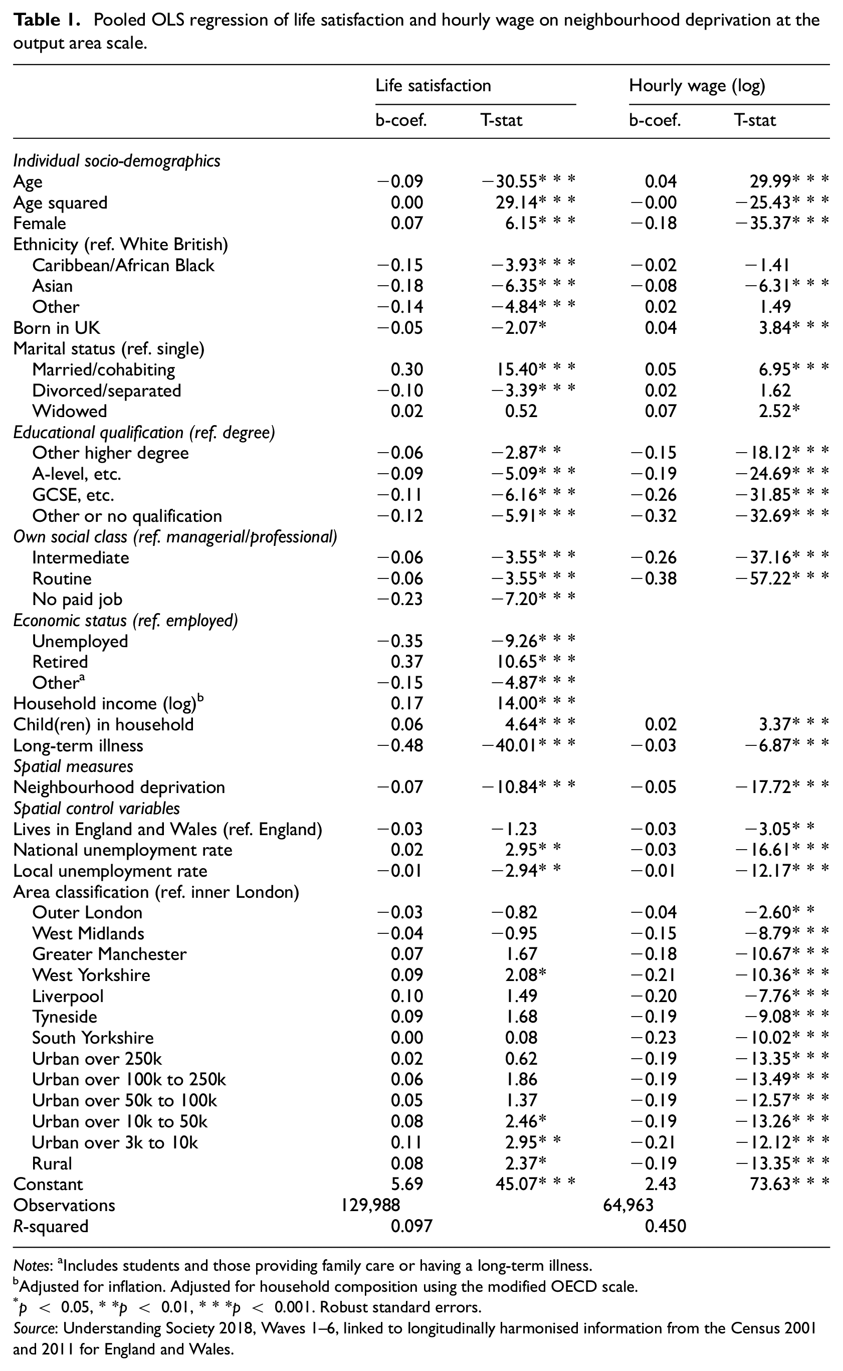
Notes: ^aIncludes students and those providing family care or having a long-term illness.

Adjusted for inflation. Adjusted for household composition using the modified OECD scale.

p < 0.05, **p < 0.01, ***p < 0.001. Robust standard errors.

Source: Understanding Society 2018, Waves 1–6, linked to longitudinally harmonised information from the Census 2001 and 2011 for England and Wales.

Consistent with previous research, we find that life satisfaction is U-shaped in age and negatively associated with minority ethnic group membership, unemployment, lower levels of income, education and poorer health (Diener et al., 1999; Knies et al., 2016; Layard et al., 2014). Earnings are positively associated with age, higher levels of education, higher-status occupations and majority ethnic group membership, as predicted by labour and education economics. The majority of factors influence life satisfaction and earnings in the same way. Stark contrasts are found across the two outcomes for the additional spatial control variables. We find that living in West Yorkshire and living in areas with a population of less than 50k are associated with satisfaction gains compared with living in Inner London. Hourly wages, by contrast, are significantly higher in London and they are particularly low in some of the areas that had comparatively high life satisfaction (e.g. West Yorkshire and small towns of 3k–10k population). While local unemployment is associated with lower life satisfaction and wages, national unemployment is associated with higher life satisfaction and lower wages. The patterns are robust to swapping the scale at which neighbourhood deprivation is measured and to accounting for different sources of unobserved heterogeneity (see Supplemental Material A3–A6, available online).

Table 2 reports the effect of neighbourhood deprivation as we swap the deprivation index at the OA level for that of the nearest 500 through 10k neighbours (top to bottom) and as we include additional controls for different sources of unobserved heterogeneity (left to right).

Table 2.

Regression of life satisfaction and log hourly wage on neighbourhood deprivation at varying neighbourhood scales and controlling for varying sources of unobserved heterogeneity.

		Pooled OLS	+ Initial conditions	+ Individual fixed effects		+ Neighbour-hood fixed effects
				$ϑ$	$γ$
Life satisfaction
OA 2001	b-coef.	−0.07	−0.07	−0.06	0.01	0.00
	T-stat	−10.84	−10.11	−3.91	0.82	−0.07
	p-value	0.000	0.000	0.000	0.414	0.948
Bespoke 500	b-coef.	−0.07	−0.06	−0.06	0.01	0.04
	T-stat	−10.42	−9.68	−3.46	0.55	0.75
	p-value	0.000	0.000	0.001	0.579	0.451
Bespoke 1k	b-coef.	−0.06	−0.06	−0.06	0.02	0.08
	T-stat	−9.94	−9.20	−3.84	1.06	1.29
	p-value	0.000	0.000	0.000	0.291	0.196
Bespoke 2k	b-coef.	−0.06	−0.06	−0.04	0.00	0.04
	T-stat	−9.55	−8.82	−2.58	−0.11	0.62
	p-value	0.000	0.000	0.010	0.912	0.533
Bespoke 3k	b-coef.	−0.05	−0.05	−0.04	0.00	0.09
	T-stat	−8.39	−7.68	−2.47	0.17	1.43
	p-value	0.000	0.000	0.014	0.868	0.153
Bespoke 4k	b-coef.	−0.05	−0.04	−0.04	0.01	0.06
	T-stat	−7.75	−7.07	−2.60	0.47	0.95
	p-value	0.000	0.000	0.009	0.637	0.341
Bespoke 5k	b-coef.	−0.05	−0.04	−0.04	0.01	0.07
	T-stat	−7.60	−6.93	−2.55	0.47	1.08
	p-value	0.000	0.000	0.011	0.640	0.279
Bespoke 6k	b-coef.	−0.04	−0.04	−0.04	0.01	0.08
	T-stat	−7.43	−6.79	−2.64	0.58	1.18
	p-value	0.000	0.000	0.008	0.563	0.240
Bespoke 7k	b-coef.	−0.04	−0.04	−0.04	0.01	0.05
	T-stat	−7.28	−6.66	−2.76	0.74	0.74
	p-value	0.000	0.000	0.006	0.458	0.459
Bespoke 8k	b-coef.	−0.04	−0.04	−0.04	0.01	0.08
	T-stat	−7.28	−6.69	−2.74	0.73	1.14
	p-value	0.000	0.000	0.006	0.466	0.254
Bespoke 9k	b-coef.	−0.05	−0.04	−0.04	0.01	0.07
	T-stat	−7.35	−6.78	−2.63	0.58	0.88
	p-value	0.000	0.000	0.009	0.559	0.380
Bespoke 10k	b-coef.	−0.05	−0.04	−0.04	0.01	0.03
	T-stat	−7.35	−6.79	−2.58	0.51	0.39
	p-value	0.000	0.000	0.010	0.610	0.698
Hourly wage (log)
OA 2001	b-coef.	−0.05	−0.04	−0.04	0.00	0.01
	T-stat	−17.72	−16.56	−9.10	−0.03	0.73
	p-value	0.000	0.000	0.000	0.980	0.463
Bespoke 500	b-coef.	−0.05	−0.04	−0.04	0.00	0.00
	T-stat	−17.64	−16.39	−8.17	−0.87	0.23
	p-value	0.000	0.000	0.000	0.384	0.821
Bespoke 1k	b-coef.	−0.04	−0.04	−0.04	0.00	−0.03
	T-stat	−16.90	−15.58	−7.68	−0.52	−1.93
	p-value	0.000	0.000	0.000	0.600	0.054
Bespoke 2k	b-coef.	−0.04	−0.04	−0.03	0.00	−0.03
	T-stat	−16.30	−14.96	−6.94	−0.88	−2.03
	p-value	0.000	0.000	0.000	0.378	0.043
Bespoke 3k	b-coef.	−0.04	−0.04	−0.03	−0.01	−0.02
	T-stat	−15.40	−14.12	−6.03	−1.47	−1.22
	p-value	0.000	0.000	0.000	0.142	0.221
Bespoke 4k	b-coef.	−0.04	−0.03	−0.03	0.00	−0.02
	T-stat	−14.84	−13.57	−5.87	−1.27	−1.10
	p-value	0.000	0.000	0.000	0.205	0.273
Bespoke 5k	b-coef.	−0.04	−0.03	−0.03	0.00	−0.02
	T-stat	−14.23	−12.99	−5.62	−1.18	−1.28
	p-value	0.000	0.000	0.000	0.238	0.201
Bespoke 6k	b-coef.	−0.03	−0.03	−0.02	0.00	−0.01
	T-stat	−13.39	−12.23	−5.37	−1.07	−0.86
	p-value	0.000	0.000	0.000	0.286	0.388
Bespoke 7k	b-coef.	−0.03	−0.03	−0.02	0.00	−0.02
	T-stat	−13.04	−11.93	−5.22	−1.12	−1.13
	p-value	0.000	0.000	0.000	0.264	0.259
Bespoke 8k	b-coef.	−0.03	−0.03	−0.02	−0.01	−0.01
	T-stat	−12.65	−11.61	−4.82	−1.33	−0.46
	p-value	0.000	0.000	0.000	0.183	0.649
Bespoke 9k	b-coef.	−0.03	−0.03	−0.02	−0.01	−0.02
	T-stat	−12.57	−11.55	−4.37	−1.73	−0.86
	p-value	0.000	0.000	0.000	0.083	0.392
Bespoke 10k	b-coef.	−0.03	−0.03	−0.02	−0.01	−0.02
	T-stat	−12.18	−11.15	−4.15	−1.74	−0.95
	p-value	0.000	0.000	0.000	0.082	0.344

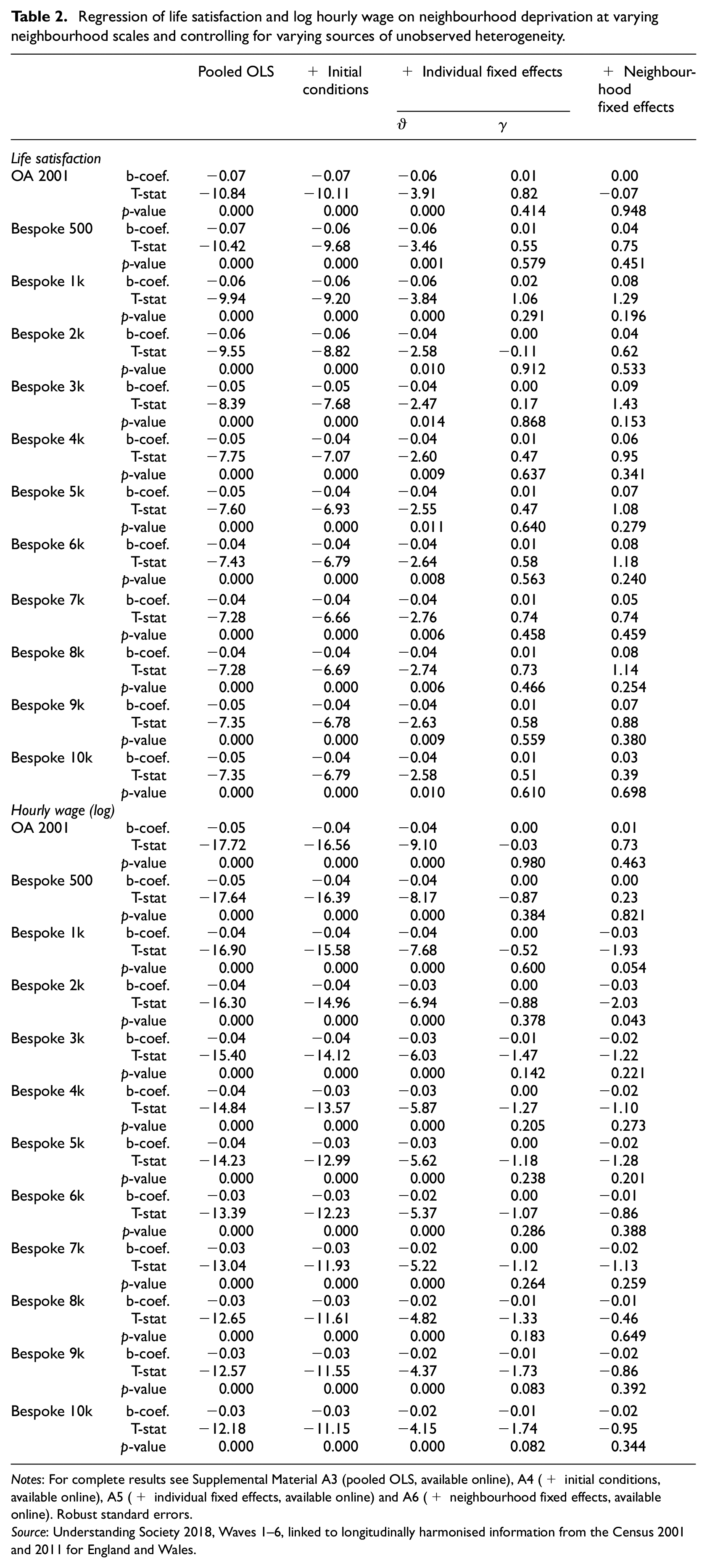
Notes: For complete results see Supplemental Material A3 (pooled OLS, available online), A4 (+ initial conditions, available online), A5 (+ individual fixed effects, available online) and A6 (+ neighbourhood fixed effects, available online). Robust standard errors.

Source: Understanding Society 2018, Waves 1–6, linked to longitudinally harmonised information from the Census 2001 and 2011 for England and Wales.

In the pooled OLS regressions, the effect of neighbourhood deprivation on life satisfaction and hourly wages is sizeable and statistically significant at all neighbourhood scales and for both outcomes: individuals who live in more deprived neighbourhoods are less satisfied with life overall and they also earn less. A standard deviation increase in deprivation is associated with a 4–7% reduction in life satisfaction and a 3–5% reduction in hourly wages. There is little evidence of variation in effect sizes across scales.

Accounting for initial conditions slightly attenuates the neighbourhood effect coefficients, suggesting that parental social class at age 14 and own social class in the first job after leaving full-time education account for some degree of heterogeneity in life satisfaction and earnings. As before, there is little evidence of variation in effect sizes across scales.

Absorbing unobserved individual effects attempts to address endogeneity bias resulting from residential sorting on individual unobserved time-invariant characteristics. It also allows us to disentangle the longitudinal (within) effect, which shows how individual wellbeing co-varies with changes in the level of deprivation experienced, from the cross-sectional (between) effect, which reports how wellbeing varies by level of neighbourhood deprivation. Consistent with the OLS results, for the cross-sectional effects (ϑ) we observe negative and statistically significant associations between deprivation and both wellbeing outcomes, particularly at smaller scales. However, there is no empirical support for the conjecture that individuals may become more satisfied or earn more as they experience a reduction in deprivation (or vice versa): All within estimates (γ) fail to reach conventional levels of statistical significance.⁷

By additionally including neighbourhood fixed effects, we can account for time-invariant unobserved heterogeneity at both the neighbourhood and individual levels. We observe clear variation in the size of the deprivation coefficient across spatial scales, particularly for life satisfaction. The results are largely in line with those from the previous less restrictive models: Deprivation is positively related to life satisfaction and negatively to wages. Accounting for unobserved time-invariant neighbourhood characteristics results in a marked yet statistically insignificant increase in the magnitude of the effect on life satisfaction. Overall, neither the effects nor the differences across scales are statistically significant.⁸

Robustness tests

We conducted several robustness tests to assess the stability and validity of the results. Figure 1 contrasts the coefficients from the pooled OLS estimates for the ‘less selected’ social renters with the coefficients obtained from estimations that account for individual- and neighbourhood-level sources of unobserved heterogeneity in the full sample (top panel) and the ‘more selected’ sample of private renters (bottom panel). Results for life satisfaction and earnings are presented in the left and right panel, respectively.

Figure 1.

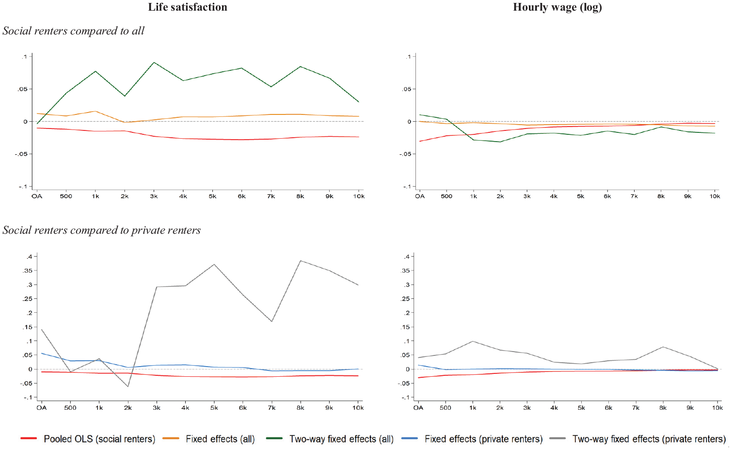
Plot of the effect of neighbourhood deprivation on life satisfaction and hourly wage at different scales of neighbourhood. Comparison of pooled OLS coefficients for social renters with coefficients from one- and two-way fixed effects models for the population as a whole (all), and private renters.

The top-right panel of Figure 1 shows that the full-sample parameter estimates of the individual- and two-way fixed effects models compare relatively well with those obtained from the pooled OLS in the sample of social renters (except at the smallest spatial scale). This lends some support to the approach of correcting for residential sorting on time-invariant individual- and neighbourhood-specific unobserved characteristics. While the panel shows an apparent variation in the effect size across spatial scales, the effect of deprivation on earnings for social renters is statistically significant only at scales up to 2k people. Although the plot suggests there are differences in patterns across the two wellbeing outcomes, in statistical terms they are the same. The effect of deprivation on life satisfaction is not statistically significant in any of the three estimations (i.e. pooled OLS for social renters compared with individual- and two-way fixed effects for the full sample) and there is virtually no variation in the effect sizes across spatial scales.

The bottom panels compare the same estimations for the sample of private renters. Concerning earnings, we observe that the parameter estimates from the social renters’ pooled OLS and the private renters’ individual fixed effects models are generally similar to each other (except at the smallest neighbourhood scale). This indicates that correcting for residential sorting on individual-specific unobserved characteristics using the correlated random effects estimator works well in removing spatial sorting bias. However, the parameter estimates for the private renters’ two-way fixed effects model exhibit a very different pattern (although the coefficients are only marginally statistically significant at the scale of 1k people (p-value = 0.053)). This, in turn, suggests that there may be other, time-variant, neighbourhood-specific characteristics confounded with area deprivation that are not accounted for in the restricted sample. We observe a similar pattern for the parameter estimates from the life satisfaction models (albeit the coefficients are not statistically significant).

Overall, the robustness tests provide empirical support for our empirical identification strategy, which combines rich longitudinal information on individual characteristics with panel data estimators that can address residential sorting on time-invariant individual-specific unobserved characteristics, as well as, to a lesser extent, on neighbourhood-specific conditions.

Discussion and conclusion

Reflecting the interdisciplinary nature of the neighbourhood effects debate and the desire for reliable causal evidence across a range of policy areas (Layard, 2005; van Ham and Manley, 2012), this paper set out to compare the effect of neighbourhood deprivation on life satisfaction and earnings, thus synthesising separate works of literature that have reached quite different conclusions regarding which neighbourhood scale matters for wellbeing, and whether or not more affluent neighbours promote wellbeing. We used rich panel data linked with longitudinal and scalable information from census records for England and Wales to examine how neighbourhood effects vary across scales and outcomes and applied various methods to address the identification challenges arising from the non-random selection of individuals and families into neighbourhoods.

We find negative associations between neighbourhood deprivation and both earnings and life satisfaction. However, this is largely due to non-random selection into neighbourhoods and not a genuine causal effect. Unlike previous studies we find no evidence for variation in the size of the association across neighbourhood scales (across all model specifications). More specifically, by adopting a stepwise approach to examining the role of different sources of unobserved heterogeneity we could show that the selection bias in our cross-sectional models is predominantly due to unobserved time-invariant individual characteristics rather than unobserved time-invariant neighbourhood characteristics. This is indicated by the reduction in the neighbourhood effect when we controlled for heterogeneity in initial conditions and more so when we additionally absorbed individual fixed effects. The sizeable and statistically significant negative cross-sectional effect differed significantly (in statistical terms, in the life satisfaction models at all neighbourhood scales and at scales below the 3k threshold in the wage models) from the longitudinal effect, which was essentially zero. Additional absorbing of neighbourhood-specific time-invariant effects did not appear to affect the results.

While the results corroborate findings from quasi-experimental studies, the fixed effects approach may not be sufficient to account for all sources of non-random selection. By focusing on social renters, who in the British context may be assumed to have a highly restricted choice over where to live, we showed that sorting bias may be appropriately removed by controlling for individual and neighbourhood fixed effects. The observed patterns of neighbourhood effects amongst social renters matched those observed in the full sample when selection on unobserved individual and neighbourhood characteristics were taken into account. However, differences between the one- and two-way fixed effects models also indicate that there is additional confounding, specifically due to time-varying neighbourhood-specific characteristics. While we cannot address empirically the issues of additional sources of unobserved heterogeneity, doing so would not likely change the main conclusion from our analyses, that is, the effect of neighbourhood deprivation on life satisfaction and earnings is largely explained by strong spatial sorting mechanisms and not a genuine causal effect.

These findings have important implications for policymaking. Notably, targeting resources specifically on neighbourhoods that are characterised by high levels of deprivation may not be a more efficient way to improve residents’ wellbeing than targeting individuals or households in need irrespective of where they live (Kline and Moretti, 2014; Melo, 2017). A focus on disadvantaged individuals may also be more effective for social justice and equity because no one is excluded from support on the basis of their neighbourhood not qualifying for area-based support. Improvements in wellbeing may be achieved through policies that, for example, increase long-term employment opportunities available to disadvantaged individuals, develop regional labour markets through better connected and more affordable transport networks, or raise skill levels. This conclusion is not, of course, an appeal for policymakers to dismiss any neighbourhood-basis for policy intervention: Given the strong correlation between neighbourhood deprivation and concentration of disadvantaged groups, local targeting can still be effective in reaching large numbers of people in need.

Our analysis is not without limitations. First, we could examine only a limited set of neighbourhood characteristics, summarised in the Townsend Deprivation Index. The use of different, more precise and timelier measures of the current and recent neighbourhood context may yield different results. More nuanced indicators may also provide an opportunity to disentangle specific effect mechanisms that may operate simultaneously at multiple scales, and which may be cancelling each other out. Of particular interest is the examination of effects on adolescents, for whom self-selection into neighbourhoods is not likely to be a source of bias and mechanisms such as socialisation and parental control are likely to operate more intensely. To our knowledge, no studies of neighbourhood effects on adolescents have adopted a bespoke neighbourhood approach to ascertain the underlying mechanisms. Second, we focused on contemporaneous neighbourhood effects and did not examine, for example, whether living in a neighbourhood that remains privileged over years or living in an area that has recently undergone gentrification makes a difference to wellbeing. Instead, our analyses show whether, and to what extent, deprivation in an average neighbourhood affects an average person. Third, our paper assumes a linear relation between neighbourhood deprivation and two wellbeing outcomes but further work is to be done regarding possible non-linear neighbourhood effects and concentrating on a greater range of outcomes that may be the focus of policy interventions.

Supplemental Material

sj-xlsx-1-usj-10.1177_0042098020956930 – Supplemental material for Neighbourhood deprivation, life satisfaction and earnings: Comparative analyses of neighbourhood effects at bespoke scales

Supplemental material, sj-xlsx-1-usj-10.1177_0042098020956930 for Neighbourhood deprivation, life satisfaction and earnings: Comparative analyses of neighbourhood effects at bespoke scales by Gundi Knies, Patricia C Melo and Min Zhang in Urban Studies

Footnotes

Acknowledgements

The research benefited from comments and feedback received on findings presented in seminars held at University of Bristol, University of Manchester, University College of London and Department for Business, Energy and Industrial Strategy (BEIS). Our particular thanks go to Maarten van Ham, Rich Harris and the other members of our project advisory team.

Declaration of conflicting interests

The author(s) declared no potential conflicts of interest with respect to the research, authorship and/or publication of this article.

Funding

We gratefully acknowledge funding from Nuffield Foundation (grant number DLW/42989). The data processing benefited from Gundi Knies’ heavy involvement in geographical data linkage as part of the ESRC-funded Understanding Society project at the University of Essex (grant number ES/K005146/1).

ORCID iD

Gundi Knies

Supplemental material

Supplemental material for this article is available online.

Notes

References

Andersson

Musterd

(2010) What scale matters? Exploring the relationships between individuals’ social position, neighbourhood context and the scale of neighbourhood. Geografiska Annaler: Series B, Human Geography 92: 23–43.

Argyle

(1999) Causes and correlates of happiness. In: Kahnemann

Diener

Schwarz

(eds) Well-being: The Foundations of Hedonic Psychology. New York: Russel Sage Foundation, pp. 353–373.

Bell

Fairbrother

Jones

(2019) Fixed and random effects models: Making an informed choice. Quality & Quantity 53: 1051–1074.

Bolster

Burgess

Johnston

, et al. (2007) Neighbourhoods, households and income dynamics: A semi-parametric investigation of neighbourhood effects. Journal of Economic Geography 7: 1–38.

Brännström

(2004) Poor places, poor prospects? Counterfactual models of neighbourhood effects on social exclusion in Stockholm, Sweden. Urban Studies 41: 2515–2537.

Brännström

(2005) Does neighbourhood origin matter? A longitudinal multilevel assessment of neighbourhood effects on income and receipt of social assistance in a Stockholm birth cohort. Housing, Theory and Society 22: 169–195.

Brynin

Güveli

(2012) Understanding the ethnic pay gap in Britain. Work, Employment and Society 26: 574–587.

Buck

(2001) Identifying neighbourhood effects on social exclusion. Urban Studies 38: 2251–2275.

Chetty

Hendren

Katz

(2016) The effects of exposure to better neighborhoods on children: New evidence from the moving to opportunity experiment. American Economic Review 106: 855–902.

10.

Clark

Westergård-Nielsen

Kristensen

(2009) Economic satisfaction and income rank in small neighbourhoods. Journal of the European Economic Association 7: 519–527.

11.

Correia

(2017) Linear models with high-dimensional fixed effects: An efficient and feasible estimator. Available at: http://scorreia.com/research/hdfe.pdf

12.

Diener

Suh

Lucas

, et al. (1999) Subjective well-being: Three decades of progress. Psychological Bulletin 125: 276–302.

13.

Dietz

(2002) The estimation of neighborhood effects in the social sciences: An interdisciplinary approach. Social Science Research 31: 539–575.

14.

Diez Roux

Mair

(2010) Neighborhoods and health. Annals of the New York Academy of Sciences 1186: 125–145.

15.

Dittmann

Goebel

(2010) Your house, your car, your education: The socioeconomic situation of the neighborhood and its impact on life satisfaction in Germany. Social Indicators Research 96: 497–513.

16.

Dujardin

Goffette-Nagot

(2010) Neighborhood effects on unemployment? A test à la Altonji. Regional Science and Urban Economics 40: 380–396.

17.

Dujardin

Peeters

Thomas

(2009) Neighborhood effects and endogeneity issues. CORE paper. Universit Catholique de Louvain.

18.

Duncan

Connell

Klebanow

(1997) Conceptual and methodological issues in estimating causal effects of neighbourhoods and family conditions on individual development. In: Brooks-Gunn

Duncan

Aber

(eds) Neighbourhood Poverty: Context and Consequences for Children. New York: Russel Sage Foundation, pp. 219–250.

19.

Durlauf

(2004) Neighborhood effects. In: Henderson

Jacques-François

(eds) Handbook of Regional and Urban Economics. Amsterdam: Elsevier, pp. 2173–2242.

20.

Friedrichs

Galster

Musterd

(2003) Neighbourhood effects on social opportunities: The European and American research and policy context. Housing Studies 18: 797–806.

21.

Galster

(2005) Neighborhood Mix, Social Opportunities, and the Policy Challenges of an Increasingly Diverse Amsterdam: Wibaut Lecture. Amsterdam: AMIDSt.

22.

Galster

(2008) Quantifying the effect of neighbourhood on individuals: Challenges, alternative approaches and promising directions. Schmollers Jahrbuch 128: 7–48.

23.

Galster

(2012) The mechanism(s) of neighbourhood effects: Theory, evidence, and policy implications. In: van Ham

Manley

Bailey

, et al. (eds) Neighbourhood Effects Research: New Perspectives. Dordrecht: Springer Netherlands, pp. 23–56.

24.

Galster

Andersson

Musterd

, et al. (2008) Does neighborhood income mix affect earnings of adults? Journal of Urban Economics 63(3): 858–870.

25.

Galster

Andersson

Musterd

(2015) Are males’ incomes influenced by the income mix of their male neighbors? Explorations into nonlinear and threshold effects in Stockholm. Housing Studies 30(2): 315–343.

26.

Hedman

Manley

Van Ham

, et al. (2015) Cumulative exposure to disadvantage and the intergenerational transmission of neighbourhood effects. Journal of Economic Geography 15: 195–215.

27.

Hedman

van Ham

Manley

(2011) Neighbourhood choice and neighbourhood reproduction. Environment and Planning A: Economy and Space 43: 1381–1399.

28.

Johnston

Jones

Burgess

, et al. (2004) Scale, factor analyses, and neighborhood effects. Geographical Analysis 36: 350–368.

29.

Kline

Moretti

(2014) People, places, and public policy: Some simple welfare economics of local economic development programs. Annual Review of Economics 6: 629–662.

30.

Knies

(2012) Income comparisons among neighbours and satisfaction in East and West Germany. Social Indicators Research 106: 471–489.

31.

Knies

(2013) Neighbourhood social ties. British Journal of Sociology 64: 425–452.

32.

Knies

Burgess

Propper

(2008) Keeping up with the Schmidts. Schmollers Jahrbuch 1: 75–108.

33.

Knies

Melo

Zhang

(2020) Neighbourhood effect studies of subjective and objective wellbeing (2002–2018). Mendeley Data V1. DOI: 10.17632/nkf79rtfk8.1.

34.

Knies

Nandi

Platt

(2016) Life satisfaction, ethnicity and neighbourhoods. Social Science Research 60: 110–124.

35.

Layard

(2005) Happiness: Lessons from a New Science. London: Penguin.

36.

Layard

Clark

Cornaglia

, et al. (2014) What predicts a successful life? A life-course model of well-being. Economic Journal 124: F720–F738.

37.

Lindahl

(2011) A comparison of family and neighborhood effects on grades, test scores, educational attainment and income – Evidence from Sweden. The Journal of Economic Inequality 9: 207–226.

38.

Manski

(1995) Identification Problems in the Social Sciences. Cambridge, MA: Harvard University Press.

39.

Mellander

Stolarick

Lobo

(2017) Distinguishing neighbourhood and workplace network effects on individual income: Evidence from Sweden. Regional Studies 51(11): 1652–1664.

40.

Melo

(2017) People, places and earnings differentials in Scotland. Regional Studies 51: 389–403.

41.

Mundlak

(1978) On the pooling of time series and cross section data. Econometrica 46: 69–85.

42.

O’Regan

Quigley

(1996) Effects upon unemployment outcomes: The case of New Jersey teenagers. New England Economic Review 3: 41–58.

43.

Petrovic

van Ham

Manley

(2019) Freedom from the tyranny of neighbourhood: Rethinking sociospatial context effects. Progress in Human Geography 44(6): 1103–1123.

44.

Platt

Knies

Luthra

, et al. (in press) Understanding society at 10 years. European Sociological Review. DOI: 10.1093/esr/jcaa031.

45.

Propper

Burgess

Bolster

, et al. (2007) The impact of neighbourhood on the income and mental health of British social renters. Urban Studies 44: 393–415.

46.

Propper

Jones

Bolster

, et al. (2005) Local neighbourhood and mental health: Evidence from the UK. Social Science & Medicine 61: 2065–2083.

47.

Sampson

Morenoff

Gannon-Rowley

(2002) Assessing ‘neighborhood effects’: Social processes and new directions in research. Annual Review of Sociology 28: 443–478.

48.

Sharkey

Elwert

(2011) The legacy of disadvantage: Multigenerational neighborhood effects on cognitive ability. American Journal of Sociology 116: 1934–1981.

49.

Shields

Price

Wooden

(2009) Life satisfaction and the economic and social characteristics of neighbourhoods. Journal of Population Economics 22: 421–443.

50.

Sutherland

Brunton-Smith

Jackson

(2013) Collective efficacy, deprivation and violence in London. The British Journal of Criminology 53: 1050–1074.

51.

Talen

(2019) Neighborhood. New York: Oxford University Press.

52.

Townsend

Phillimore

Beattie

(1988) Health and Deprivation: Inequality and the North. London: Routledge.

53.

University of Essex, ISER, et al. (2018) Understanding Society: Waves 1–8, 2009–2017 and Harmonised BHPS: Waves 1–18, 1991–2009. Colchester: UK Data Service.

54.

van Ham

Manley

(2012) Neighbourhood effects research at a crossroads: Ten challenges for future research. Environment and Planning A: Economy and Space 44: 2787–2793.

55.

van Ham

Boschman

Vogel

(2018) Incorporating neighborhood choice in a model of neighborhood effects on income. Demography 55: 1069.

56.

Weinhardt

(2014) Social housing, neighborhood quality and student performance. Journal of Urban Economics 82: 12–31.

Supplementary Material

Please find the following supplemental material available below.

For Open Access articles published under a Creative Commons License, all supplemental material carries the same license as the article it is associated with.

For non-Open Access articles published, all supplemental material carries a non-exclusive license, and permission requests for re-use of supplemental material or any part of supplemental material shall be sent directly to the copyright owner as specified in the copyright notice associated with the article.

0.00 MB

0.26 MB

Neighbourhood deprivation,life satisfaction and earnings: Comparative analyses of neighbourhood effects at bespoke scales

Abstract

Keywords

Introduction

Neighbourhood effects: Identification challenges and empirical findings

Identification challenges

Neighbourhood effects on life satisfaction

Neighbourhood effects on earnings

Empirical strategy

Modelling framework

Robustness tests

Data

Individual wellbeing outcomes and control variables

Bespoke neighbourhoods and spatial controls

Results

Full sample results

Robustness tests

Discussion and conclusion

Supplemental Material

sj-xlsx-1-usj-10.1177_0042098020956930 – Supplemental material for Neighbourhood deprivation, life satisfaction and earnings: Comparative analyses of neighbourhood effects at bespoke scales

Footnotes

Acknowledgements

Declaration of conflicting interests

Funding

ORCID iD

Supplemental material

Notes

References

Supplementary Material