Automated draping analysis of 3D printed flexible isogrid structures for textile applications

Abstract

Fused filament fabrication (FFF) 3D printing can be used for manufacturing flexible isogrid structures. This work presents a novel draping analysis of flexible 3D printed isogrids from thermoplastic polyurethane (TPU) using image processing. A small-scale multi-camera automated draping apparatus (ADA) is designed and used to characterize draping behavior of 3D printed isogrid structures based on draping coefficient (DC) and mode. Circular specimens are designed and 3D printed that accommodate up to eight additional weights on their perimeters to enhance draping. Five infill patterns, three infill percentages, and three loading cases are explored to evaluate their impact on specimens’ draping coefficient and mode, resulting in 45 tests. The range of DCs in this study is 21.9% to 91.5%, and a large range of draping modes is observed. For the lowest infill percentage, specimen mass is not the sole contributor to the DC values and the infill pattern has a significant impact for the three loading cases. Considering draping modes, the maximum number of convex and concave nodes observed for 25% infill specimens with added weights is three. The draping behavior characterization developed in this study can be followed to design and 3D print new flexible isogrids with textile applications.

The topic of fabric drape has been an ongoing area of research in engineering for nearly a century. Traditionally, fabric drape is the ability of a textile to deform under the force of gravity. Fabric drape was once solely described as a subjective and qualitative attribute of a textile, which led to inconsistencies in its description. Several studies began to emerge with the goal of objectively and quantitatively assessing the draping characteristics of textiles. Early studies include a fabric strip bending test devised by Pierce ¹ in 1930. This test simply measured the amount of displacement observed for a clamped section of fabric with a given length due to bending deformation. Meanwhile at an MIT textile research laboratory, Schiwarz et al. ² tested a newly developed drape tester known as the Drape-o-meter. This simple apparatus consisted of a rectangular fabric specimen with a given length suspended vertically. A disk with a circumference equal to twice the fabric width was physically attached at the top of the specimen to deform the fabric into a semi-circle. A second coincident disk located at the base of the apparatus was used to measure the amount of departure from curvature the fabric specimen exhibited. The radius of curvature was used to quantify the relative stiffness and therefore drapeability of different textiles. A high curvature is exhibited in a material with high drapeability and a low curvature is exhibited in a stiff material. Later studies aimed to quantify three-dimensional draping behaviors to better improve draping analysis. In 1950, Chu et al. ³ performed a study with a new drapemeter developed by their Fabric Research Laboratories in Massachusetts. The F.R.L. drapemeter was an optical based system which projected the draped profile of a circular specimen sandwiched between two circular plates onto a glass surface. This draped profile was hand-traced on an annular ring of tracing paper and its enclosed area was determined. The draping coefficient (DC) was conceptualized as the projected 2D draped area divided by the total area of the annular ring. This dimensionless draping parameter allows different textiles to be compared quantitatively. A textile with a higher DC is said to have a lower drapability compared to a textile with a lower DC. With this basic relationship, a perfectly stiff material would have a DC of 100% and a theoretically perfect drape would have a DC of 0%. An improved F.R.L. drapemeter was developed during the same study after identifying errors in determining an accurate draping coefficient by as much as 17%. In addition, the improved apparatus automatically plotted the outline of the draped specimen using a pen attached to the output of a mechanical linkage. The draped area was calculated using a planimeter by tracing the perimeter drawn by the apparatus. This significantly improved the drapemeter by automating the tracing process and reducing the error caused by the previous system. In 1962, Cusick et al. ⁴ began developing a new drapemeter which adopted the circular specimen and circular plates from the F.R.L. drapemeter. However, Cusick’s drapemeter utilized a parabolic mirror and a light source instead of a lens to accurately project the shadow of the draped area. The shadow was hand-traced by the user and a planimeter was used to determine the area and final DC. Cusick initially used 18-cm and 30-cm diameter textiles, which corresponded to a range in DC of 30% to 98%. In 1965, Cusick ⁵ further studied the behavior of fabric drape with focus on the dependency on the bending and shear stiffness of the fabric. In 1968, Cusick ⁶ proposed three sample dimensions: 24, 30, and 36 cm in diameter. A new method to determine the DC was proposed by cutting the outline of the traced area and weighing it. The weight ratio was used to determine the area of the draped specimen to reduce time spent using a planimeter.

The aforementioned studies required the user to be skilled at operating each apparatus, and the manual procedures were time consuming. As imaging and computing technology improved, several studies began to emerge with a common goal to automate and improve existing manual drapemeters.^7–9 The fundamental drapemeter architecture and concepts remained the same; however, a digital camera was used to capture an image of the projected draped area. Image processing software was developed and used to calculate the draping coefficient and other parameters. The main draping parameter of interest remained as the DC, but additional features such as mode, i.e., the number of folded pleats and their shape, were also tabulated. Early studies focused on the validation of image processing technology for replacing the existing manual techniques. Kenkare et al. ¹⁰ found that image analysis techniques accurately determined DC using the accepted weight ratio method as a baseline. Mei et al. ¹¹ developed a unidirectional fabric drape testing method to generate a 3D model of a vertically draped curtain using a single depth camera. Hussain et al. ¹² , ¹³ developed a medium-scale draping apparatus using multiple depth cameras to image a statically draped fabric from different angles. A point cloud was generated and used to create a 3D model of the draped specimen, but resulted in an average dimensional error of 2–3 cm. This study also investigated the ability to digitally slice the draped surface into ten sections to reveal the draping mode of the fabric drape. It should be noted that there have been several studies dedicated to accurately modeling draped textiles using finite element modeling. Hedfi et al. ¹⁴ summarized the work of previous studies which accurately simulate dynamic drape behavior using appropriate equations describing the anisotropic material properties.

The 3D printing process has been used to manufacture parts for a wide range of applications including textiles. Initial studies focused on the use of conventional non-flexible materials, e.g., polylactic acid (PLA) and acrylonitrile butadiene styrene (ABS), to manufacture rigid woven structures. ¹⁵ Some studies attempt to mimic drapability via interlocked structures, for example, chainmail, using both fused filament fabrication (FFF) and selective laser sintering printing technologies. ¹⁶ , ¹⁷ Spahiu et al. ¹⁸ investigated the ability to vary fabric drape by 3D printing PLA patterns directly onto the surface of a fabric. The fabric used was 0.67-mm-thick polyester and 0.46-mm-thick polyamide, and they concluded that the 3D printed patterns significantly influenced the DC but less strongly influenced the number of nodes visualized. Several other investigations focused on printing standard materials like PLA and Taulman 645 Nylon on textiles, and many report issues with adhesion to the fabric.^19–21 However, previous studies have not yet quantified draping behavior of 3D printed textiles. In addition, the use of thermoplastic elastomers (TPEs), such as thermoplastic polyurethane (TPU) and ethylene vinyl acetate (EVA), remains absent in the literature for this application.

Several studies have investigated the mechanical properties of TPEs, such as TPU and EVA. Nakajima et al. ²² investigated the use of kirigami structures to improve the load-carrying capability and elongation of flexible specimens from printed TPU with Shore hardness 91A. The impact of stacking sequence, slit size, and thickness on the tensile properties was investigated. Out-of-plane deformation perpendicular to the applied tensile load was observed to significantly improve the percent elongation at failure. The maximum tensile strength and percent elongation at break was found to be 2.43 MPa and 183%, respectively. Xiao et al. ²³ developed a medical grade TPU filament using a single-screw extruder, and tensile coupons were 3D printed. The maximum tensile strength and percent elongation at break was found to be 46.7 MPa and 702%, respectively. Kumar et al. ²⁴ , ²⁵ investigated the optimal printing parameters for EVA and reported a maximum tensile strength and percent elongation at break of 8.83 MPa and 522%, respectively. Other studies investigate the wear behavior, thermal properties, adhesive properties, shape-memory, and dimensional considerations of TPU during 3D printing.^26–30 These hyper-elastic materials exhibit very high elongation for a given applied load and behave unlike elastic materials which deform linearly. The material characterization, especially drapeability of 3D printed components manufactured from flexible materials from various TPEs, e.g., TPU, remains very limited in the literature.

In this study, drapeability of flexible isogrid structures printed with FFF from TPU is investigated. A multi-camera automated draping apparatus (ADA) is designed and built to measure draping coefficient, and record draping mode for different 3D printed flexible isogrids. Circular specimens with a diameter of 10 cm with five infill patterns and three infill percentages are 3D printed for testing. To enhance and amplify the inherent draping behavior of isogrid specimens, four and eight 1.5-g weights are added on their perimeters. Draping coefficients and modes are compared for specimens with different infill patterns and percentages, for given loading cases: with and without additional weights. The article wraps up with closing remarks and recommendations for future research.

Methodology

Figure 1 represents the procedure of the automated draping analysis from the specimen manufacturing to the draping analysis. This iterative procedure can be utilized to rapidly design, prototype, and characterize the draping behavior of 3D printed isogrid structures.

Figure 1.

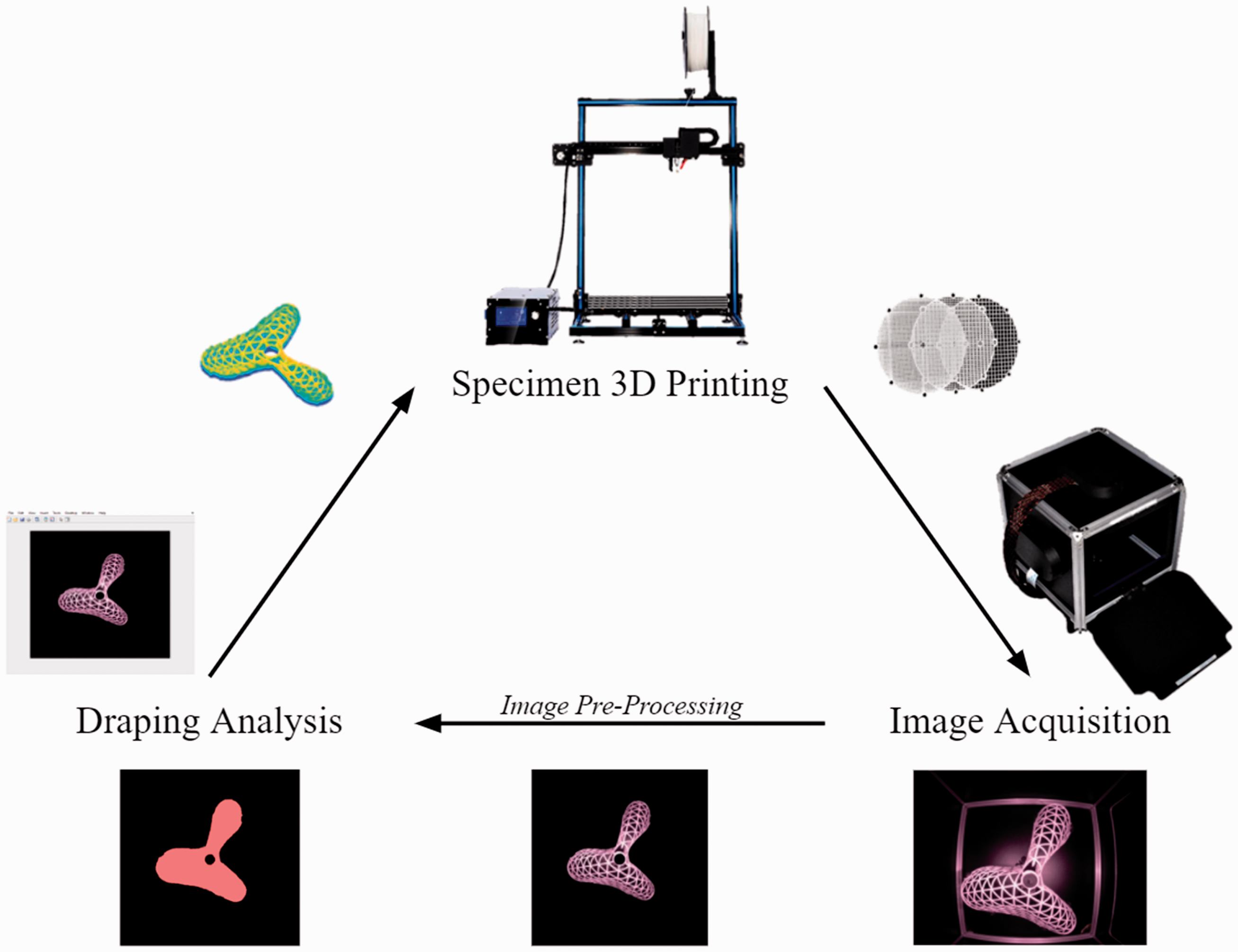
Overview of 3D printed isogrids draping analysis.

Specimen geometry

Figure 2 shows the 10-cm diameter circular specimen designed to accommodate up to a maximum of eight weights on its perimeter to enhance its draping behavior. Standard metric grade 10.9 bolts and nuts were used as weights for the different loading cases. Each weight consisted of a M3 × 8 mm button head hex socket bolt and three nuts. These attachment points are located along 0°, 90°, and ±45° to simulate standard loading angles along several directions. Loading case A consists of all eight weights added (indicated by the red circles in Figure 2(b)), loading case B has four weights added in 0° and 90° (indicated by the blue circles), and there are no added weights for loading case C. Each weight has a mass of 1.5 g, which corresponds to 12 g added for loading case A and 6 g added for loading case B.

Figure 2.

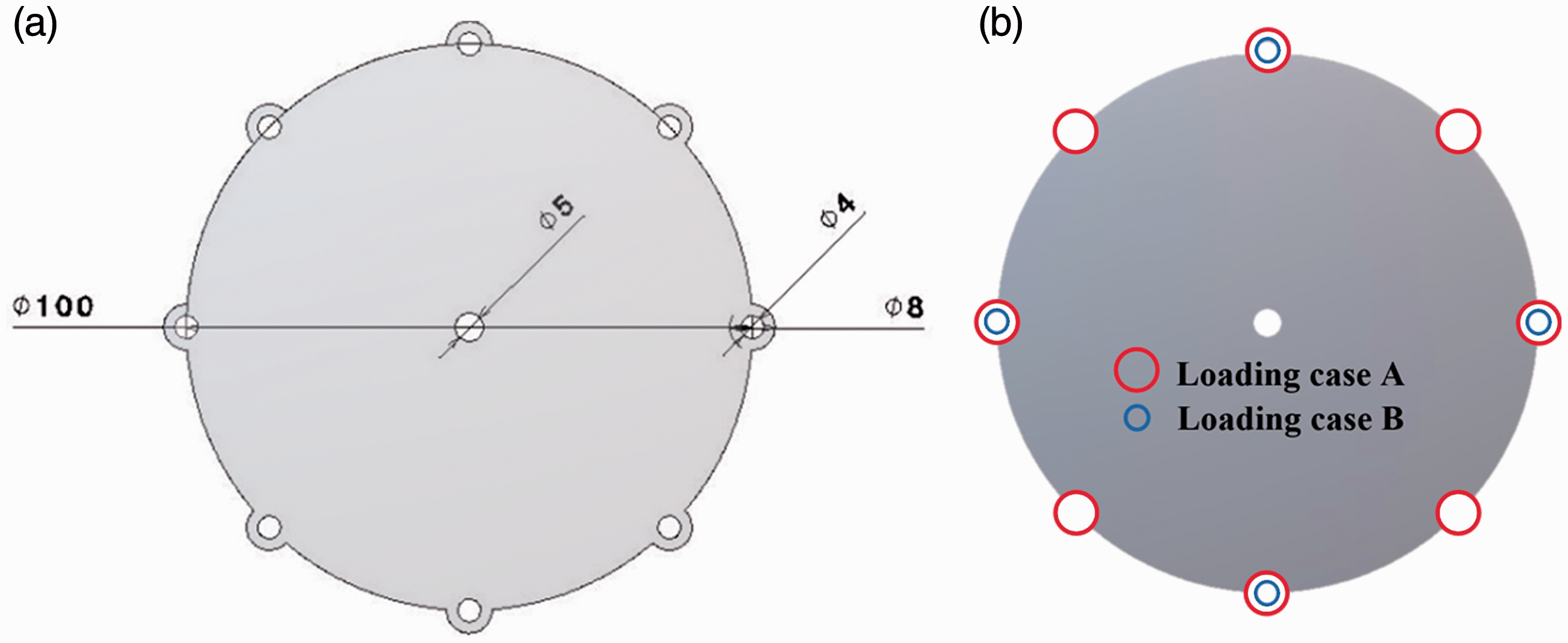
Specifications of the specimen. (a) Specimen geometry; and (b) three loading cases with extra weights in the attachment points, i.e., A: eight; B: four; and C: no extra weights.

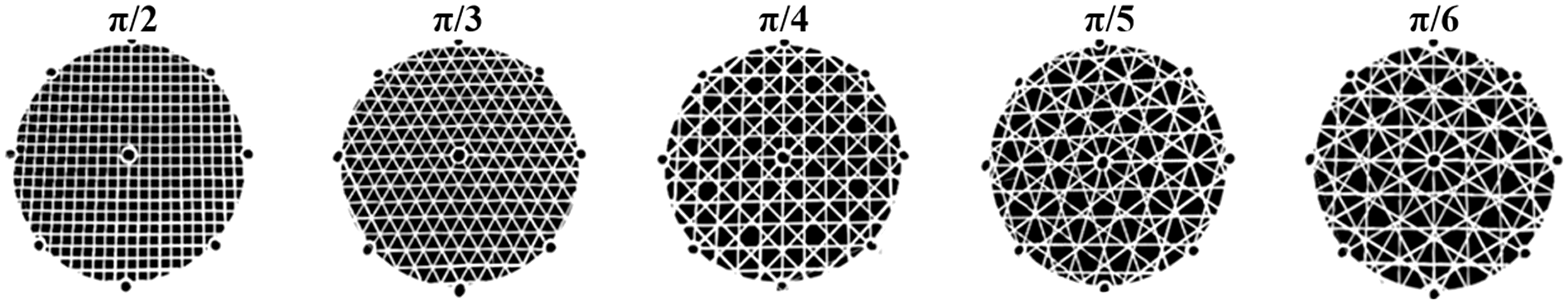
Geometric structures, e.g., isogrids, have been used for various aerospace applications in the past several decades. ³¹ These lightweight and stiff structures are typically machined from aerospace grade aluminum using large computer numerical control milling machines. However, current advancements in the composites industry allow for carbon fiber reinforced polymer isogrids to be manufactured using a rib-skin method.^32–34 An isogrid lattice composed of intersecting rib stiffeners at specific angles is interfaced with an outer skin to form an isogrid stiffened skin. In addition, a few studies have started to investigate the manufacturing of an isogrid stiffened skin structure using additive manufacturing. ³⁵ , ³⁶ Isogrid lattices can be described by a simple relation of π/m, where π is the angle in radians (or 180°) and m is the number of fibers with a unique angle. When m is equal to two (2), this is a specific case not regarded as an isogrid where the angles present are 0° and 90°. All other values of m>2 are isogrid structures with each greater value being a higher order than its predecessor. Figure 3 shows the five infill patterns investigated in this study: 0° and 90° paths (π/2, m=2); 0° and ±60° paths (π/3, m=3); 0°, ±45°, and 90° paths (π/4, m=4); 0, ±36 and ±72 paths (π/5, m=5); and 0, ±30, ±60, and 90 paths (π/6, m=6). The path angle is meaured from the positive x-axis and the counterclockwise direction is considered as positive.

Figure 3.

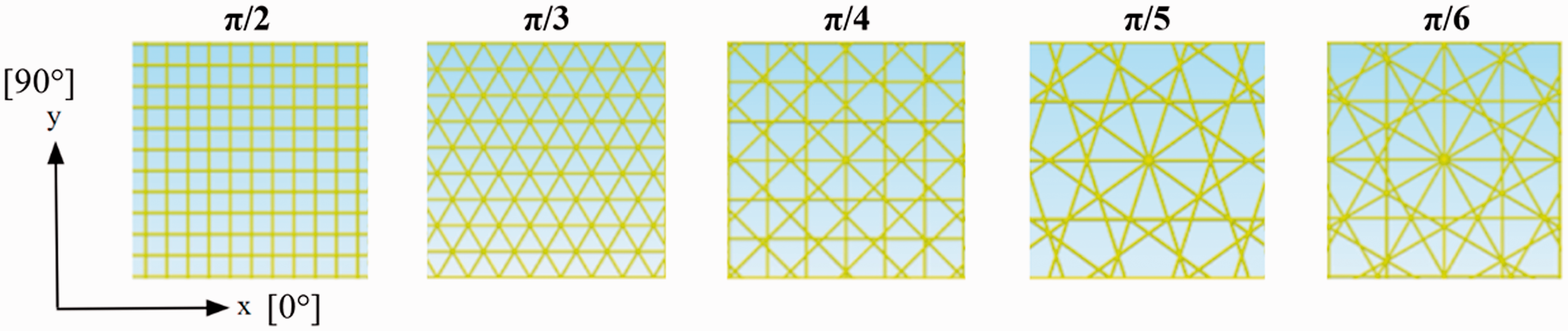
Specimen infill patterns and axis definition.

GCODE generation and specimen 3D printing

The GCODE for each specimen was generated using the Simplfy3D slicer software version 4.1.2. Figure 4 shows the complete test plan with 25% infill samples in the top row, 50% in the middle, and 75% in the bottom. Moving from left to right the value of m, which defines the type of isogrid, increases from a minimum value of two to a maximum of six.

Figure 4.

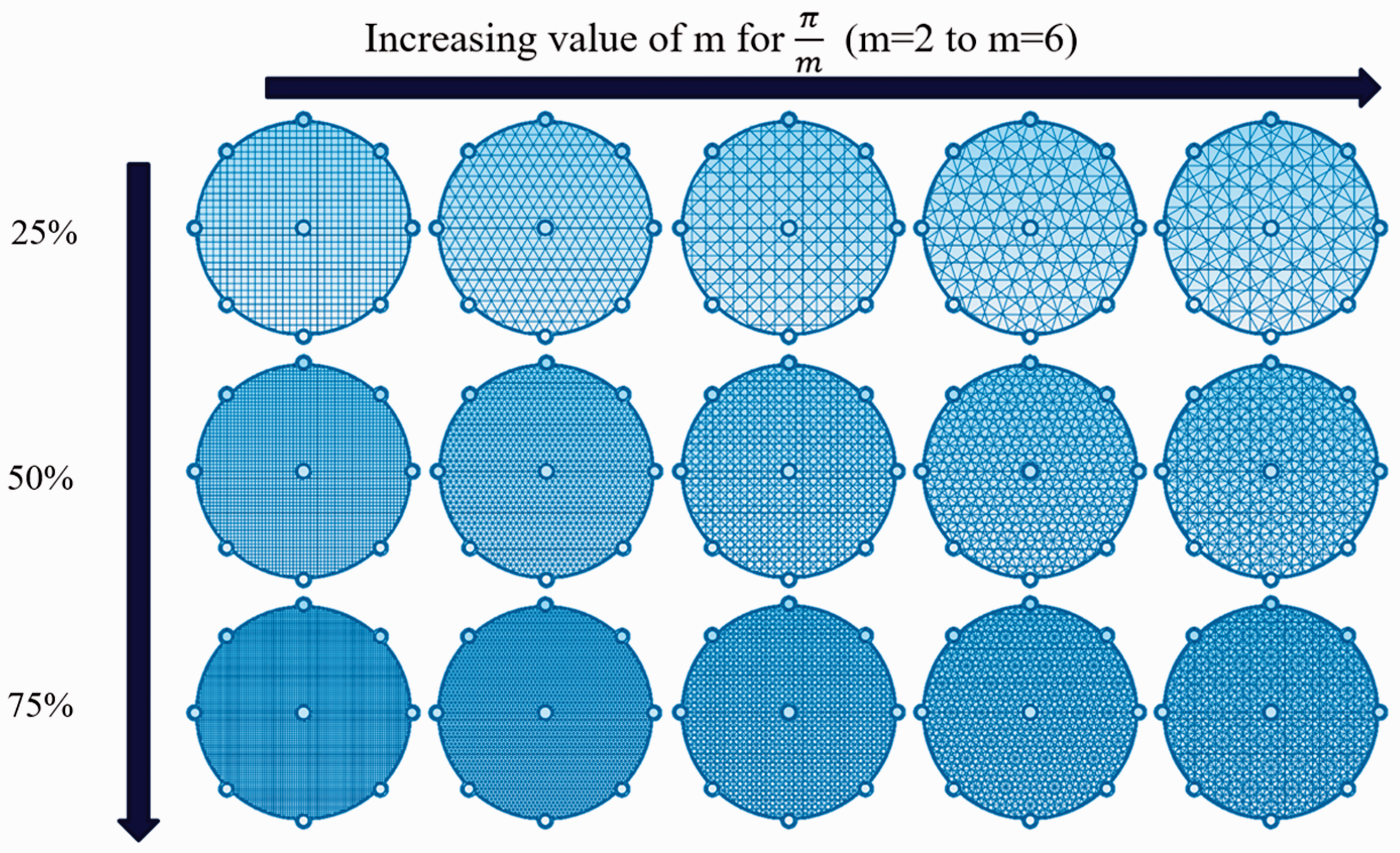
The test plan for draping analysis.

The FFF-style 3D printer selected for the specimen manufacturing was the ADIMLab 3D printer (ADIMLab, Hong Kong, China) which features a direct-drive extruder. A common printing challenge encountered with flexible filaments is a tendency to jam prior to melting in the nozzle. A standard Bowden-style extruder tends to present difficulty with flexible materials as the filament is drawn through a long polytetrafluoroethylene (PTFE) tube prior to entering the nozzle. A direct-drive extruder helps to prevent this by minimizing the distance the filament travels before entering the nozzle. In addition, the retraction of a filament throughout a print is often used to reduce print defects, e.g., stringing, due to travel moves. However, flexible filaments are often deformed when retracted and can form a kink if standard slicer settings are used. Furthermore, the overall print speed often needs to be reduced to minimize both the feed-rate of the filament and eliminate any print defects. A custom 3D printing profile was created to manufacture specimens from the flexible TPU filament successfully. The white pigmented TPU filament with Shore hardness 91A was from Filaments.ca with batch number 918018162. Table 1 summarizes the key 3D printing parameters. The infill patterns tested consist of the follow angled fibers in degrees: π/2: 0/90, π/30/60/−60, π/4 $:$ 0/90/45/−45, π/5: $$ 0/36/−36/72/−72, and π/6: 0/90/30/−30/60/−60.

Table 1.

3D printing parameters for all specimens

Manufacturing parameter	Value	Manufacturing parameter	Value
Material	TPU (91A)	Nozzle temperature	220°C
Build orientation	XYZ	Bed temperature	50°C
Raster angle	See Figure 4	Printing speed	900 mm/min
Filament diameter	1.75 mm	Infill percentage	25%, 50%, 75%
Nozzle diameter	0.4 mm	Layer height	0.25 mm

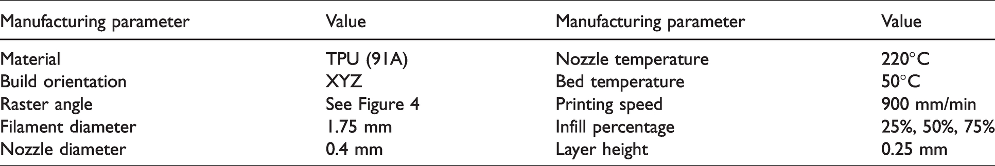
Figure 5 shows the actual 3D printed specimens from white TPU with 25% infill. It should be noted these specimens were manufactured in a single 0.25-mm layer, meaning the printed extrudates of varying raster angle intersect each other to form a unique weave pattern as shown in Figure 6(a). The number of intersections increases with infill percentage, and the number of extrudates per intersection is the integer number defining each isogrid pattern. For the π/3 specimen, the number of 3D printed extrudates at a given intersection is three (Figure 6(b) and (c)). The nozzle of the 3D printer is momentarily displaced vertically as it intersects a previously deposited extrudate, forming the stacking order observed. The number indicates the stacking order of the extrudates as they are printed as follows: (1) 0°, (2) 60°, and (3) −60°. The specimens are comprised of repeating sections of locally woven intersections, resulting in a flat textile-like structure.

Figure 5.

Top view of the actual 3D printed specimens from white TPU with 25% infill.

Figure 6.

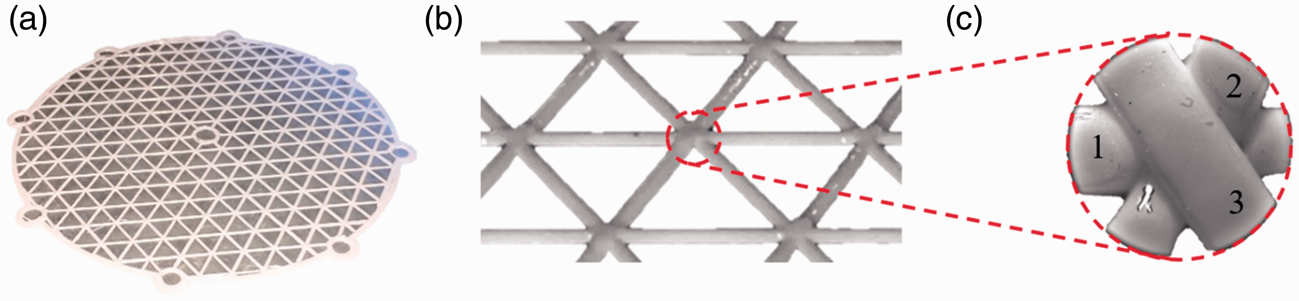
The π/3 specimen with 25% infill. (a) 3D printed specimen on the build platform; (b) a close-up of the 3D printed specimen; (c) micrograph of 3D printed extrudates intersection.

A total of 15 specimens were manufactured for testing (five for each infill percentage, see Figure 4). Figure 7 shows the measured mass of each specimen. As expected, with an increase in the infill percentage, the specimen’s mass increases significantly. Additionally, for the same infill percentage, there is a limited increase in the mass of specimens with lower m values (from m=2 to 3 and 4) compared with specimens with higher m values (from m=4 to 5 and 6).

Figure 7.

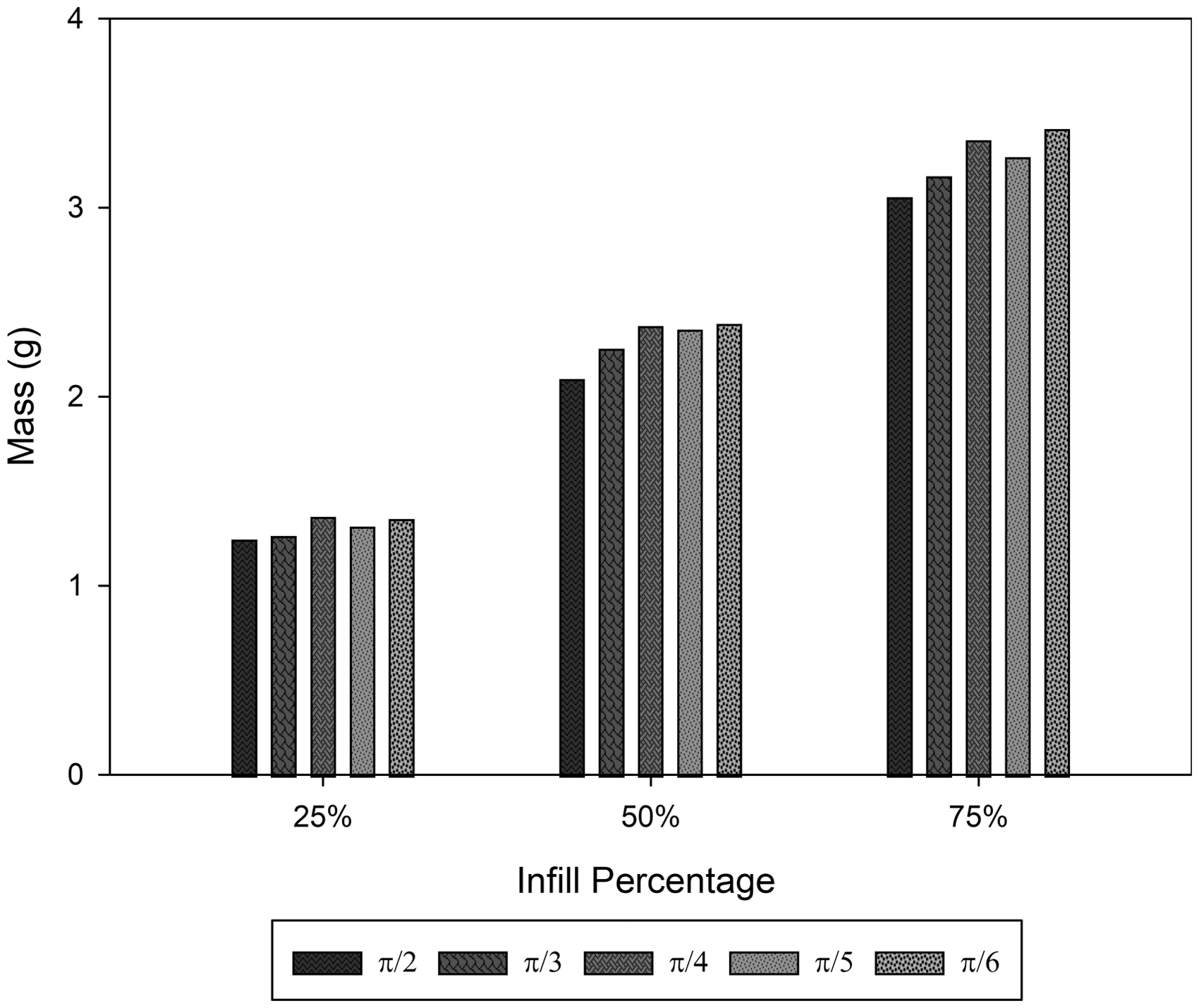
Mass of each specimen versus infill percentage.

Automated draping apparatus

A small-scale multi-camera ADA was designed in CATIA and manufactured using miniature 10 × 10 mm profile aluminum extrusion. The 150 × 150 × 150 mm enclosed apparatus features a rotating draping post and two wide-angle cameras each with two InfraRed (IR) illuminators (Figure 8). The cameras capture clear images of the draped specimen without the addition of visible light. Matte black vinyl wrap was adhered to the panels to produce high contrast between the white specimens and to aid with the image processing. The static top and side cameras combined with the central rotating post allows a draped specimen to be accurately imaged from all angles. A Python script was written to automatically photograph each draped specimen from the top and side while displaying a live video preview on a 7” touchscreen LCD using a Raspberry Pi 3. The draped specimen is rotated and photographed 12 times in 30° increments, resulting in full 360° imaging of the specimen. Rotating 360° ensured that all draped specimens were photographed in their entirety. The specimen is imaged while stationary for 2 s to ensure the photos are clear and the total testing duration is about 30 s per specimen. Since both a top and side camera are used, each specimen tested results in a total of 24 images. In Figure 8, the isometric and wireframe views of the ADA are shown with annotations describing key components and a side camera image of a draped 25% infill π/2 specimen in loading case A inside the ADA during the image acquisition.

Figure 8.

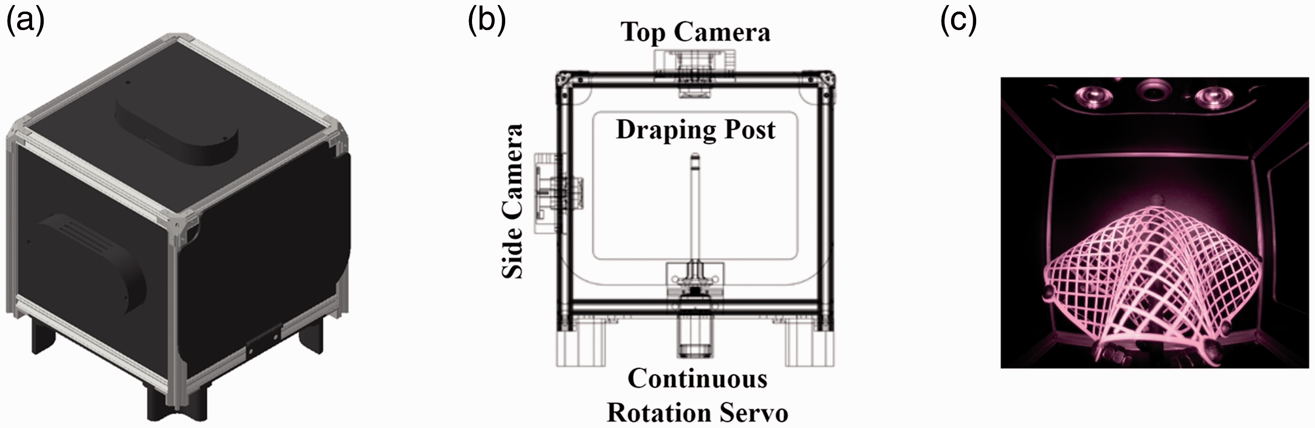
Overview of the ADA. (a) Isometric; (b) wireframe; and (c) side view with a draped π/2 specimen with 25% infill inside.

Figure 9(a) shows the actual ADA during testing, while Figure 9(b) illustrates the access door used to place each specimen on the central draping post and to prevent external visible light from entering the testing chamber.

Figure 9.

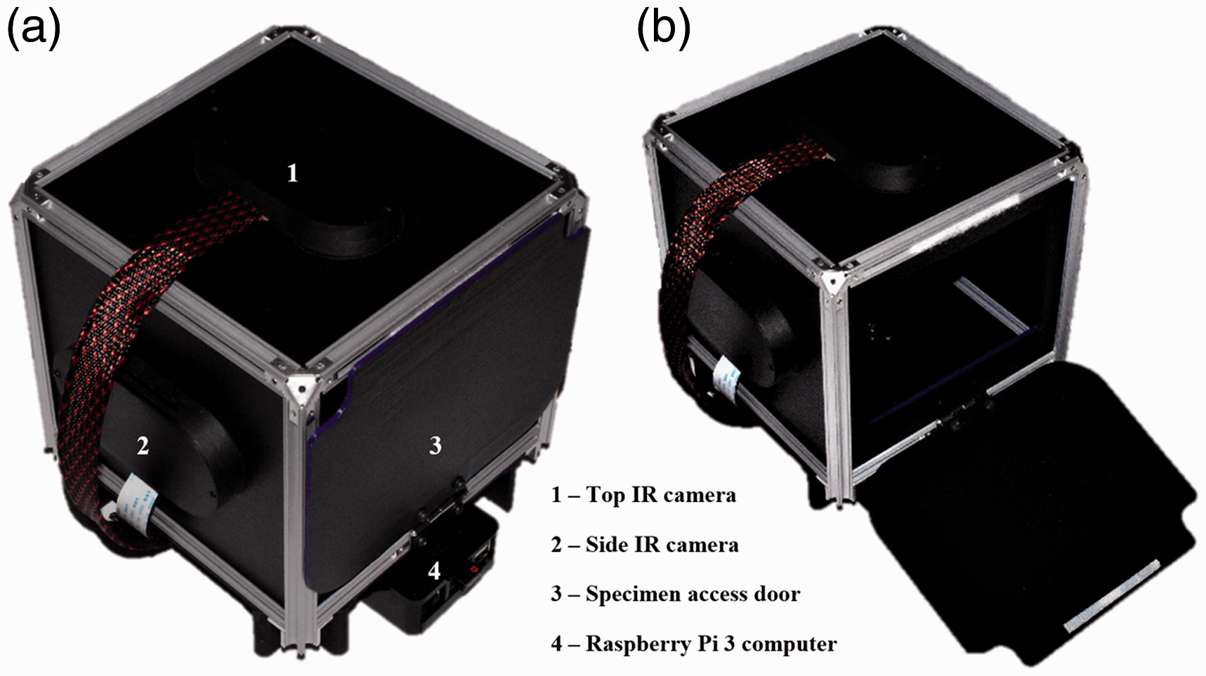
The ADA. (a) Closed access door for testing; and (b) open access door.

In Figure 10, the 7” touchscreen display used to preview the image acquisition of each draped specimen is shown. The draped specimen can be observed in real time as it is imaged.

Figure 10.

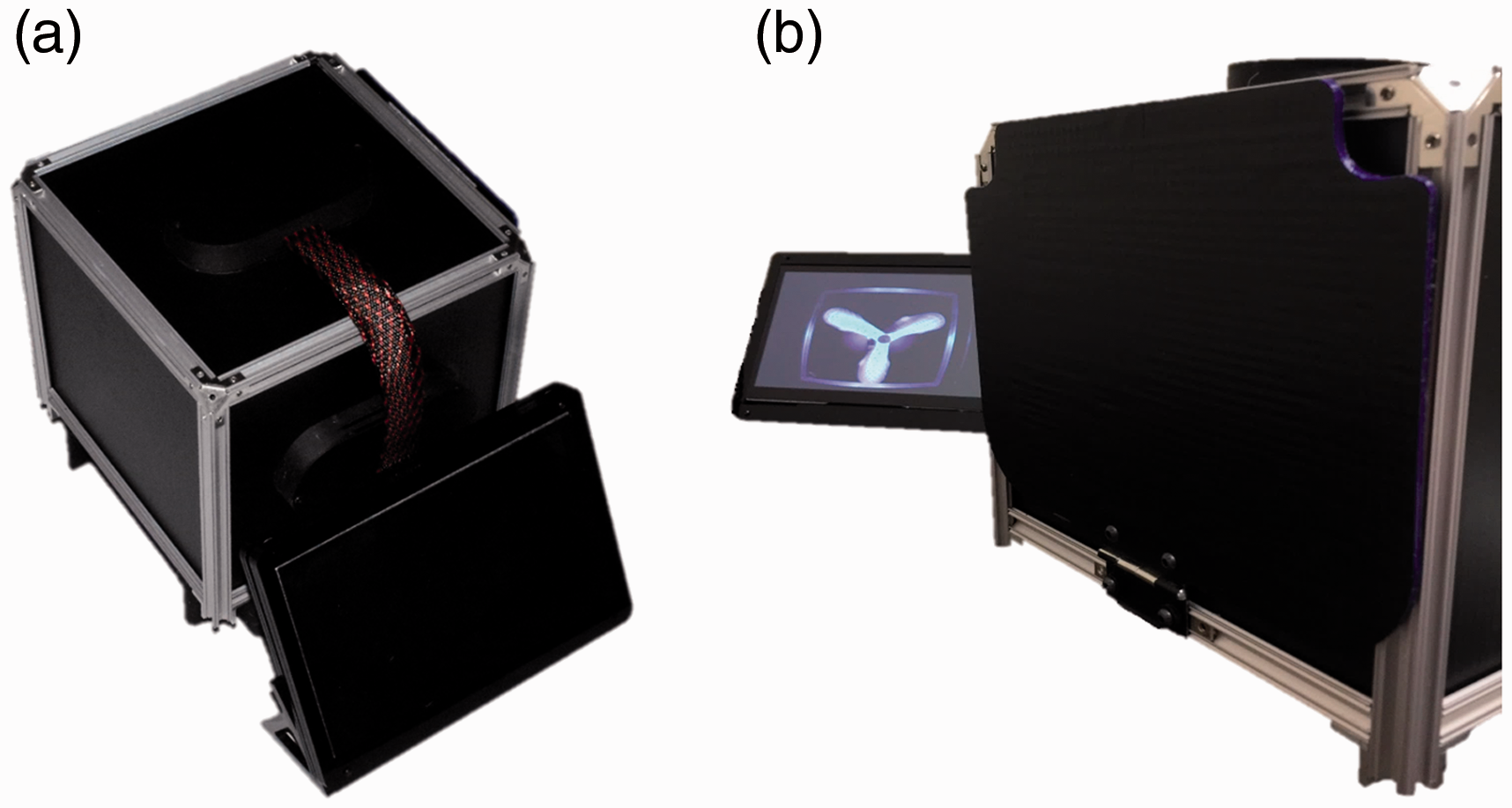
LCD display for the ADA. (a) 7” touchscreen; and (b) live preview of top view.

A MATLAB script was written to perform image processing and complete the final draping analysis. Figure 11 shows the top view of each draped specimen used for the determination of the dimensionless draping coefficient (DC) for each of the three loading cases: A, B, and C. All five isogrid patterns are shown from left to right with increasing infill percentage of 25%, 50%, and 75% from top to bottom. The 15 specimens were tested in each of the three loading cases denoted A, B, and C, resulting in a total of 45 images. Each one of these photos was selected from the 12 photos taken for the top view of each specimen and captured the draped specimen in its entirety.

Figure 11.

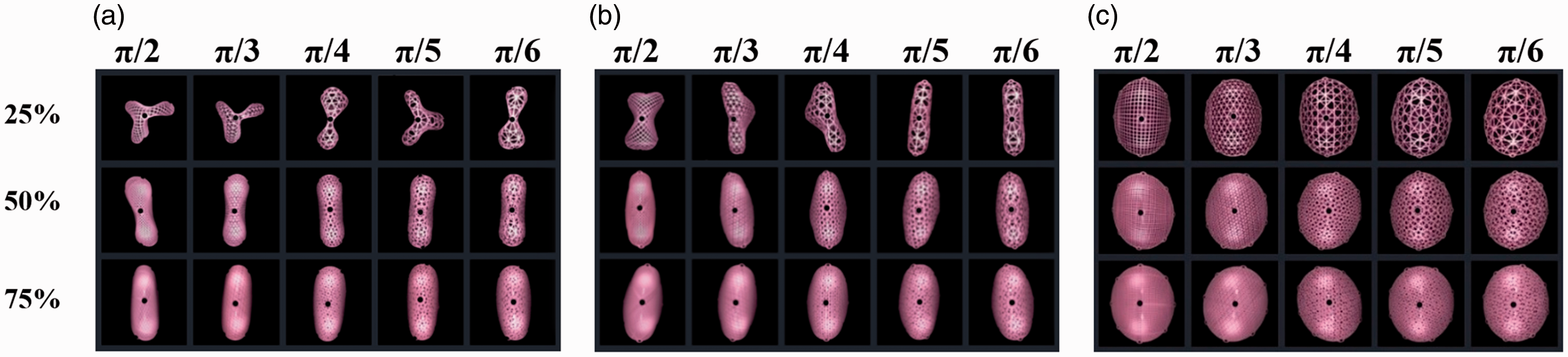
Final images of specimens used for draping analysis. (a) Loading case A; (b) loading case B; and (c) loading case C.

To determine the DC of each specimen, the surface areas measured via the image processing are input into equation (1). The .jpg format photos are converted into binary images which are used with the “bwarea” function within the Image Processing Toolbox in MATLAB to extract the draped area. Each image was cropped to 500 × 500, equally 250,000 total pixels, during pre-processing and imported into the MATLAB script to perform the draping analysis of all 45 images shown in Figure 11. The undraped area is the surface area of the 10-cm diameter circular specimen, which is equal for any pattern (see Figure 4). This area is independent of the printed pattern, as it is defined as area enclosed by the perimeter of the geometry. The undraped pixel count was determined to be 148,552, resulting in a corresponding DC of 100%. The software identifies and removes the infill pattern to calculate the pixel count of the enclosed area of each draped specimen. Dividing the draped pixel count by the constant undraped pixel count, 148,552, computes the DC of each specimen for all infill patterns under all loading conditions.

$$\mathrm{Draping}\mathrm{ }\mathrm{Coefficient}\mathrm{ }\left(\mathrm{DC}\right)=\frac{\mathrm{Draped}\mathrm{ }\mathrm{Area}}{\mathrm{Undraped}\mathrm{ }\mathrm{Area}}\times 100\mathrm{\%}=\frac{\mathrm{Draped}\mathrm{ }\mathrm{Pixel}\mathrm{ }\mathrm{Count}}{\mathrm{Undraped}\mathrm{ }\mathrm{Pixel}\mathrm{ }\mathrm{Count}}\mathrm{ }\times 100\mathrm{\%}$$

(1)

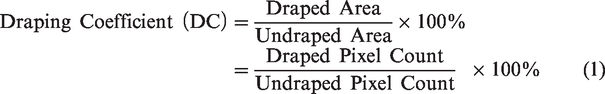
Figure 12 shows the pre-processed image, enclosed draped area, and resulting draping coefficient for the π/2 specimen with 25% infill for loading case A. The process is repeated for all 15 specimens for the three loading cases (the 45 images in Figure 11), and results are discussed in Results and discussion.

Figure 12.

Draping analysis for the π/2 specimen with 25% infill. (a) Pre-processed image; (b) draped area determination; and (c) DC output.

The MATLAB script exports the DC results to a .xlsx file which is opened using Microsoft Excel. The results shown represent the 45 tests after the ADA hardware and draping analysis software underwent calibration. In this work, the primary focus was to use the top camera to determine DC as supported by conventional draping apparatuses in the literature.^3–10 The draping modes also only require the top view of a draped specimen as the concave and convex regions result from clearly defined folded pleats. However, a side camera allows for the generation of a three-dimensional (3D) model of a draped specimen using photogrammetry software. Additional draping parameters of a given specimen, e.g., angles and areas of folded pleats, can be measured using the 3D model and can be investigated in future studies.

Results and discussion

Draping coefficient

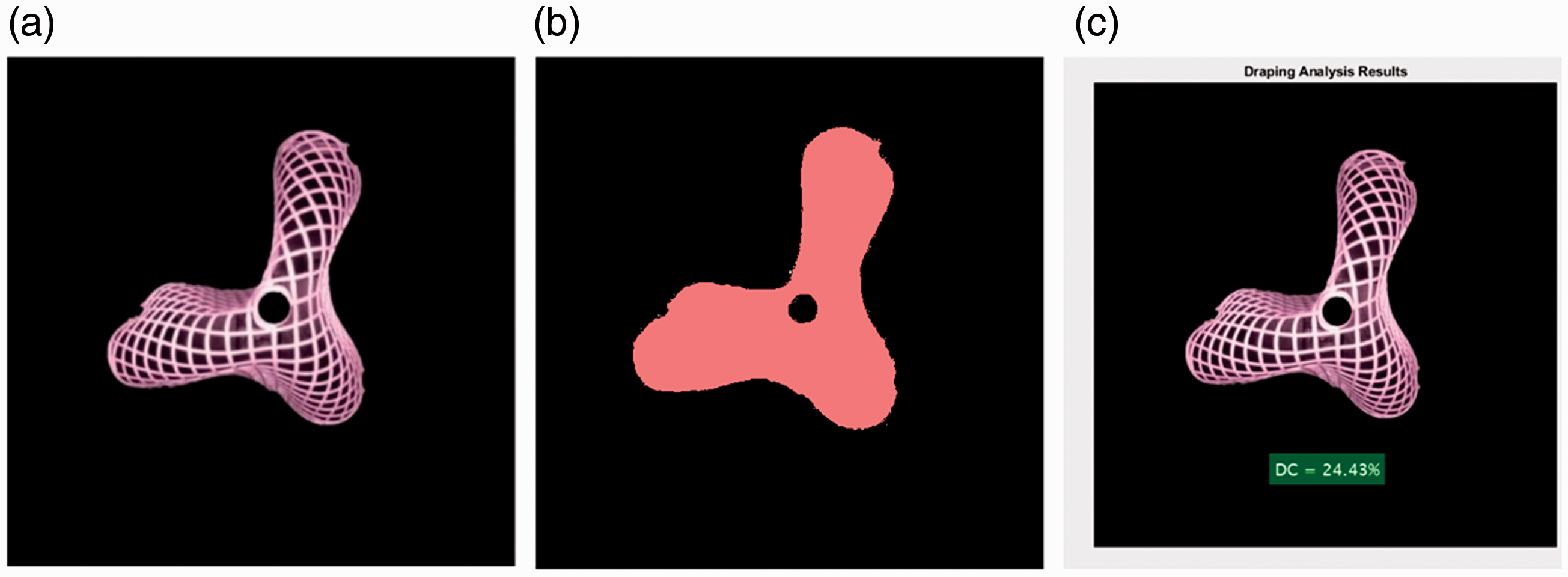
The DC of specimens depends on their infill pattern, infill percentage, and the external loading. We investigate each of these design variables separately in this section. Figures 13–15 show the impact of the infill pattern on the DC of the specimens, while Figure 16 shows the effect of the infill percentage and the loading case. Figure 13 provides a snapshot of the DC values versus the infill pattern and percentage for loading case A for all specimens. It should be recalled that loading case A has eight additional weights on the perimeter of the specimens. The π/3 specimen with 25% infill had the lowest recorded DC (21.9%), and the π/5 specimen with 25% infill had the highest value (27.2%). For both the 50% and the 75% infill cases, the π/2 specimens had the lowest DC of 36.0% and 39.9%, respectively. Lastly, the π/6 specimens had the highest DC for both 50% and 75% infill with 44.0% and 51.3%, respectively.

Figure 13.

Draping coefficient versus infill pattern and percentage for loading case A.

Figure 14.

Draping coefficient versus infill pattern and percentage for loading case B.

Figure 15.

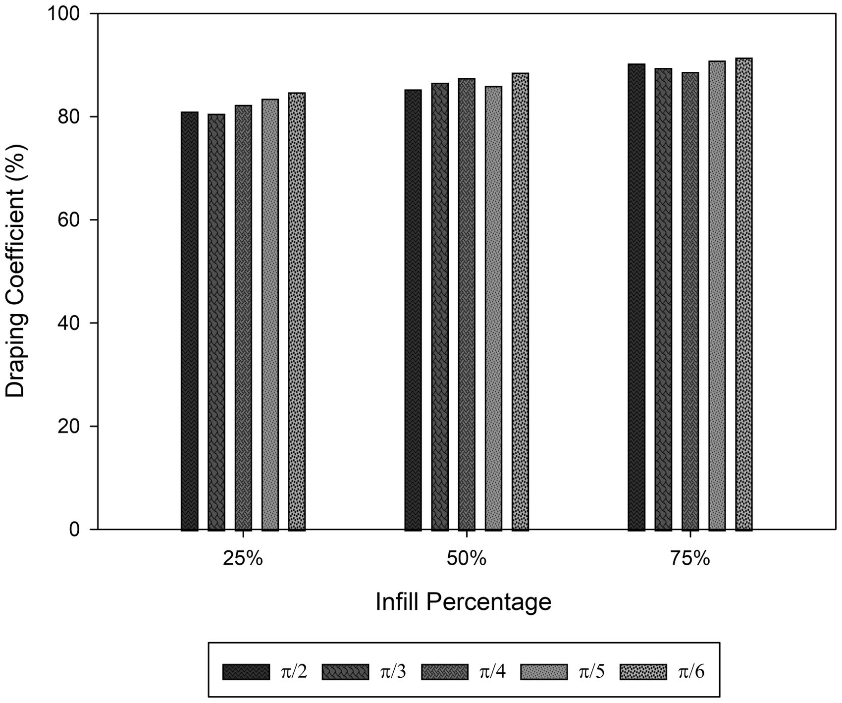
Draping coefficient versus infill pattern and percentage for loading case C.

Figure 16.

Draping coefficient for different infill patterns and loading cases versus infill percentage. (a) π/2 specimens; (b) π/3 specimens; (c) π/4 specimens; (d) π/5 specimens; and (e) π/6 specimens.

FFF 3D printing process introduces anisotropic properties to manufactured parts with tensile strength and modulus being maximum along extrudates and minimum in the transverse direction. ³⁷ , ³⁸ This means that if loading is along the extrudates of a specimen, they can resist it more compared to the transverse direction. This results in a lower deflection, lower draping, and a higher DC. It can also be concluded that the specimen is stiffer under loading along its extrudates compared to the transverse direction. At the low infill percentage of 25%, this anisotropy has significant impact on the behavior of the specimens, while at higher infill percentages, i.e., 50% and 75%, the specimen behaves more like an isotropic material. This means that the specimen does not show directional properties, and its behavior along and transverse to the extrudates are identical. This is also true when for a fixed infill percentage (e.g., 50% or 75%) the value of m in the isogrid increases from 2 to 6. The reason is that there are more extrudates in the plane of the specimens for higher m values and they behave more closely to an isotropic material, also called quasi-isotropic.

Figure 13 shows DC values for loading case A, which has eight extra weights along 0°, 90°, and ±45° angles (see Figure 2(b)). For the 25% infill, there is a significant anisotropy in the specimens and the π/2 specimen with 0° and 90° extrudates resists loading (extra weights along 0°, 90°, and ±45°) more compared to the π/3 specimen with 0° and ±60° extrudates. This results in a lower deflection and a higher DC value for the π/2 than the π/3 specimen. This is also the same reason that the π/4 specimen with 0°, 90°, and ±45° extrudates has a higher DC than the π/3 specimen. For the 25% infill, as m increases from 2 to 6, the specimens become more isotropic; therefore, the DC increases for m values of 5 and 6 since loading case A has extra weights along quasi-isotropic directions, which is 0°, 90°, and ±45° angles.

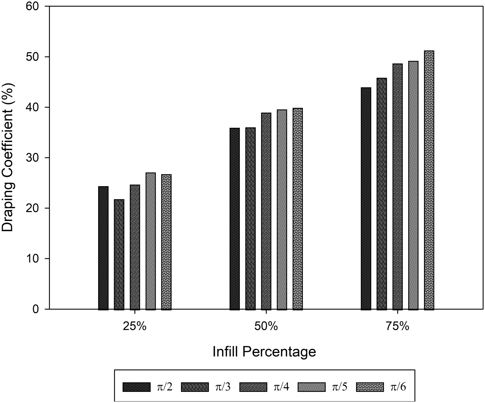
Figure 14 shows the comparison of the draping coefficient (DC) versus the infill pattern and percentage for loading case B. It should be recalled that loading case B has four additional weights on the perimeter of the specimens along 0° and 90° directions. The π/5 specimen with 25% infill had the lowest DC (34.1%), while the π/6 specimen with 75% infill had the highest DC (60.2%). For the 25% infill, the π/2 specimen had the highest DC among different infill patterns (38.7%) and is closely followed by the π/4 specimen. For this low infill percentage, there is a significant anisotropy in the specimens, and the π/2 specimen with 0° and 90° extrudates as well as the π/4 specimen with 0°, 90°, and ±45° extrudates resist loading (extra weights along 0° and 90°) more compared to the π/3 specimen with 0° and ±60° extrudates. This results in higher DC values for the π/2 and π/4 specimens compared to the π/3 specimen. For high infill percentages (50% and 75%), the specimens behave more closely to an isotropic material and there are no directional properties. As a result, at 50% and 75% infills, the impact of the specimen mass and its overall stiffness is more significant than its stiffness under specific loading conditions. The π/2 specimen has the lowest mass for 50% and 75% infill (see Figure 7), and it almost shows the lowest DC values.

Figure 15 shows the comparison of the DC versus the infill pattern and percentage for loading case C (no additional weight). The π/3 specimen with 25% infill had the lowest DC (80.7%), while the π/6 specimen with 75% infill had the highest DC (91.5%). It should be noted that the π/6 specimens exhibited the highest DC for all three of the infill percentages with no weights added. As explained before for loading cases A and B, the π/6 specimens behave closer to an isotropic material. Therefore, they can resist better their own weight and deform less compared to other isogrids, resulting in high DC values. DC values for all infill patterns and percentages are close to each other with a maximum difference of 10.8 percentage point (a minimum DC of 80.7% for the π/3 specimen with 25% infill and a maximum DC of 91.5% for the π/6 specimen with 75% infill). The range of DC values for loading case A and B is 21.9% to 51.3% and 34.1% to 60.2%, respectively. This amounts to a maximum difference of 29.4 and 26.1 percentage point for loading case A and B, respectively. As expected, the additional weights on the specimens enhanced their draping behavior and increased the range of resulting DC values.

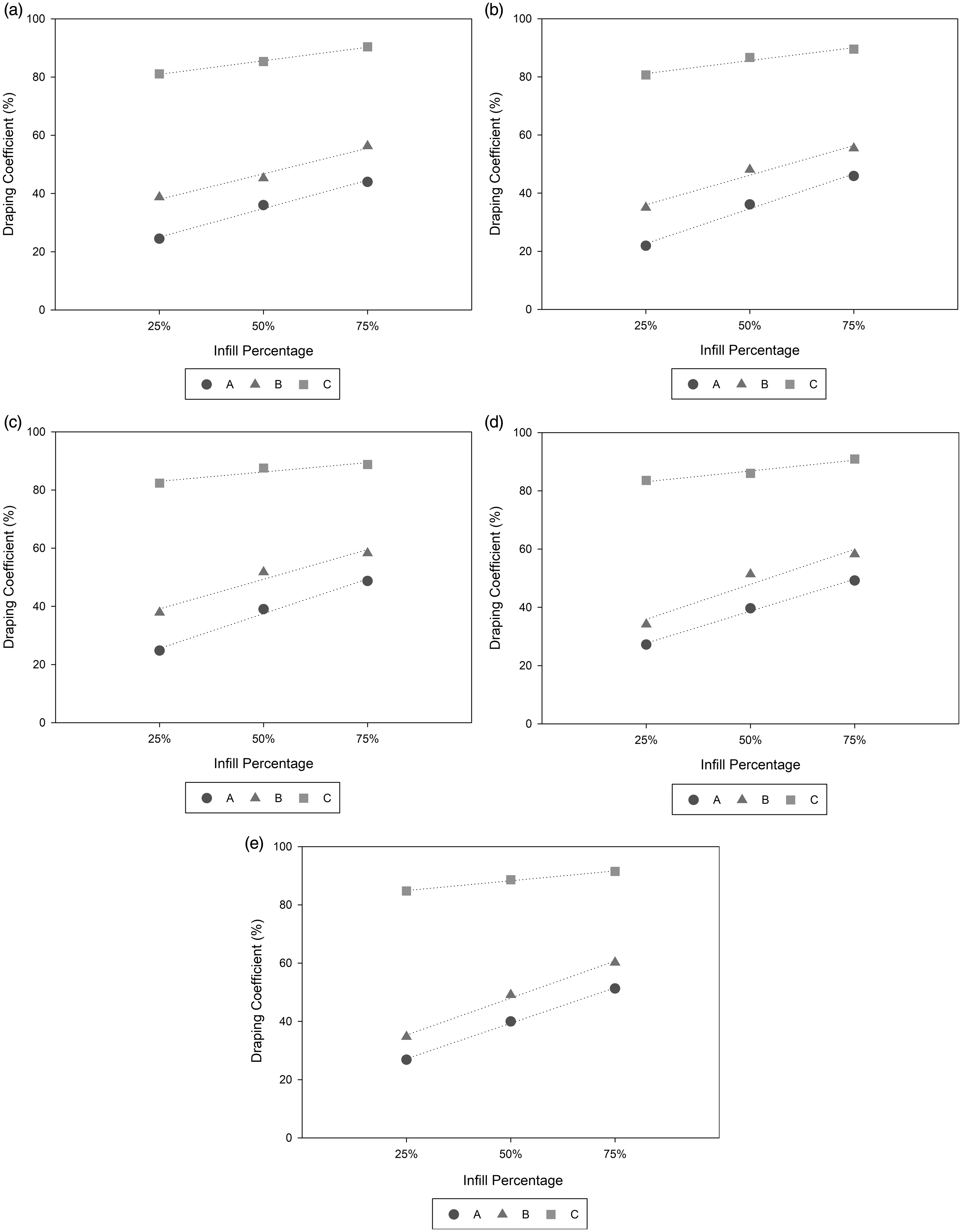
Figure 16 shows a scatter plot of the DC versus infill percentage for each of the five infill patterns for the three loading cases. A linear trendline has been added for each set of data to highlight the trends. There is almost a linear increase in DC with an increase in infill percentage for all infill patterns and loading cases. The rate of increase is almost identical among all loading cases for π/2 infill pattern, while loading cases A and B have a higher rate of increase in DC for other infill patterns, i.e. π/3, π/4, π/5, and π/6. For each additional 25% of infill added, each specimen sees a percentage point increase of over 10% in its DC. For example, the π/5 pattern most notably has the largest percentage point increase in DC for loading case B from 34.1% in DC for 25% infill to 51.4% in DC for 50% infill (an increase of 50.7%).

Draping modes

An identifiable trait of textiles, and in the case of 3D printed isogrid structures, is the presence of pleats which defines a given draping mode of a specimen as it deforms and manifests folds. These pleats can be irregular or regular and their occurrence is proportional to the size of the specimen. For loading case A, a maximum of three pleats were observed. However, the arrangement and size of these pleats varied for each of the specimens tested. To distinguish between the various draping modes, an identification pattern is proposed to assess the number of distinct rounded convex and concave pleats. A differing number of these pleats highlights any clear irregularity in the draped specimen. The draping mode classification proposed in this work is presented in equation (2).

$$\mathrm{Draping} \mathrm{Mode} \left(M\right)=\left(\#\mathrm{of} \mathrm{Convex} \mathrm{Pleats}, \#\mathrm{of} \mathrm{Concave} \mathrm{Pleats}\right)=(n_1,n_2)$$

(2)

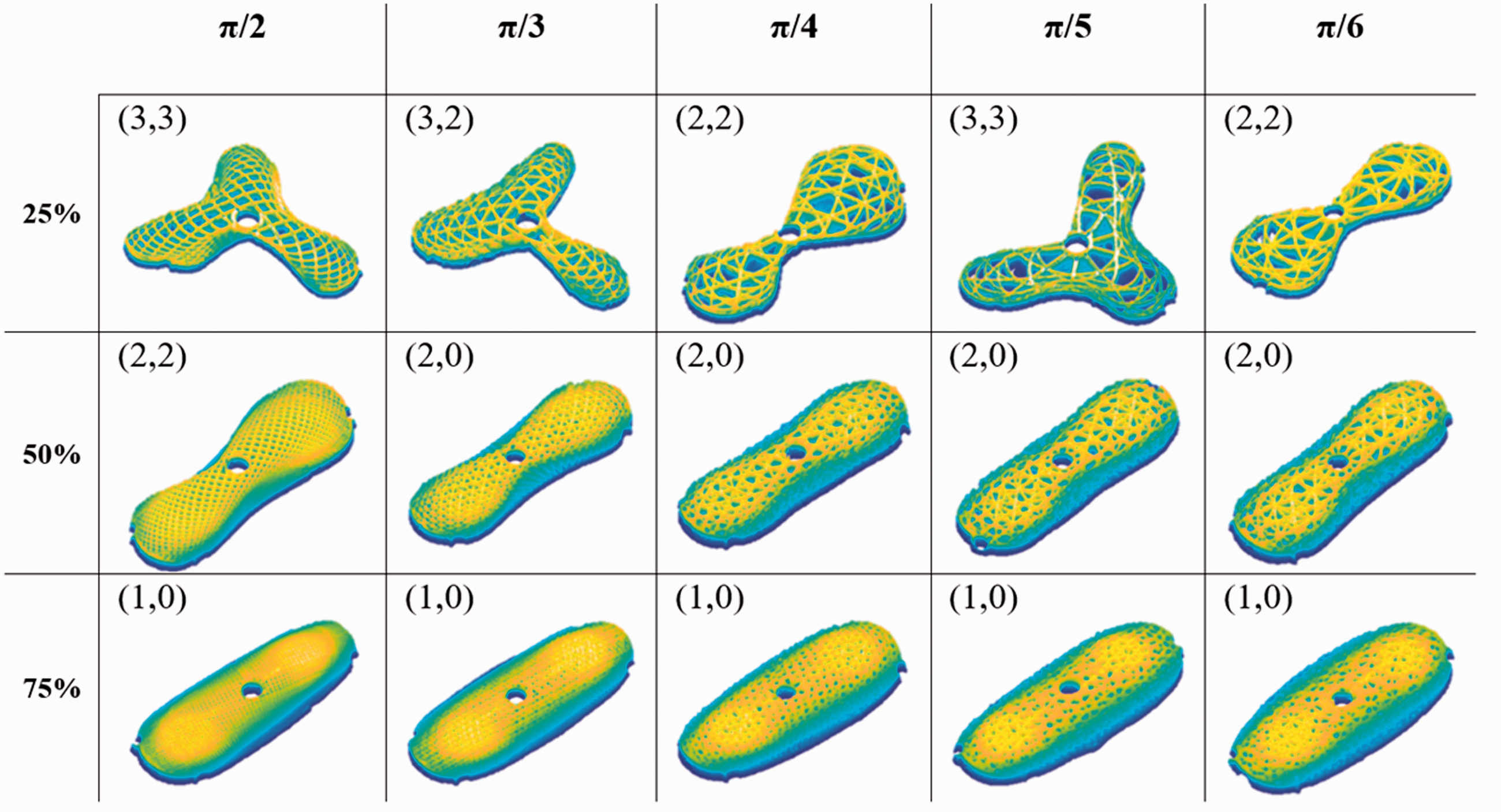
It should be noted that a qualitative assessment of the draped specimen is performed to identify convex and concave pleats. If a region cannot be categorized clearly as convex or concave, it will be denoted by a value of zero in equation (2). For example, a simple ellipse is considered to have only one distinct continuous rounded convex pleat as it is unbroken by any straight lines and thus defined as (1,0). This qualitative assessment can also be quantified using the first and second derivatives of the draped specimen regions. In this way, in addition to the DC, the image analysis software can identify the draping mode that will be considered for future work. Figure 17 shows the draping modes for loading case A, with three distinct modes observed for the 25% infill specimens. For the 50% infill specimens, two distinct modes were observed, while the specimens with 75% infill only had one deformed shape, i.e. an ellipse with a single uniform fold. In this case, their draping mode classification remained as (1,0), and these specimens can only be distinguished quantitatively using the draping coefficient (DC).

Figure 17.

Draping modes of specimens for loading case A.

Beginning with 25% infill, the π/2 specimen displayed a distinct symmetric ternary draping mode with three rounded convex and concave pleats as denoted by (3,3). Next, the π/3 specimen deformed asymmetrically with three distinct rounded convex pleats but only two distinct rounded concave pleats on the bottom right side of the image. The slightly concave region on the left side of the image cannot be categorized as a distinct rounded concave pleat. This threshold range is a qualitative assessment of the linearity of the given region. Since the local slope is nearly linear, it could not be considered a true rounded convex pleat and thus is denoted as (3,2). Next, the π/4 specimen displayed a distinct symmetric binary draping mode with two rounded convex and concave pleats as denoted by (2,2). Lastly, the π/5 specimen showed a draping mode of (3,3), like the π/2 specimen, and the π/6 specimen had a similar draping mode to the π/4 specimen. Most specimens with 50% infill showed two distinct rounded convex pleats, (2,0), while all specimens with 75% infill deformed in a manner of an ellipse with a single uniform fold. In this case, their draping mode classification remained as (1,0), and these specimens are best distinguished quantitatively using the draping coefficient (DC).

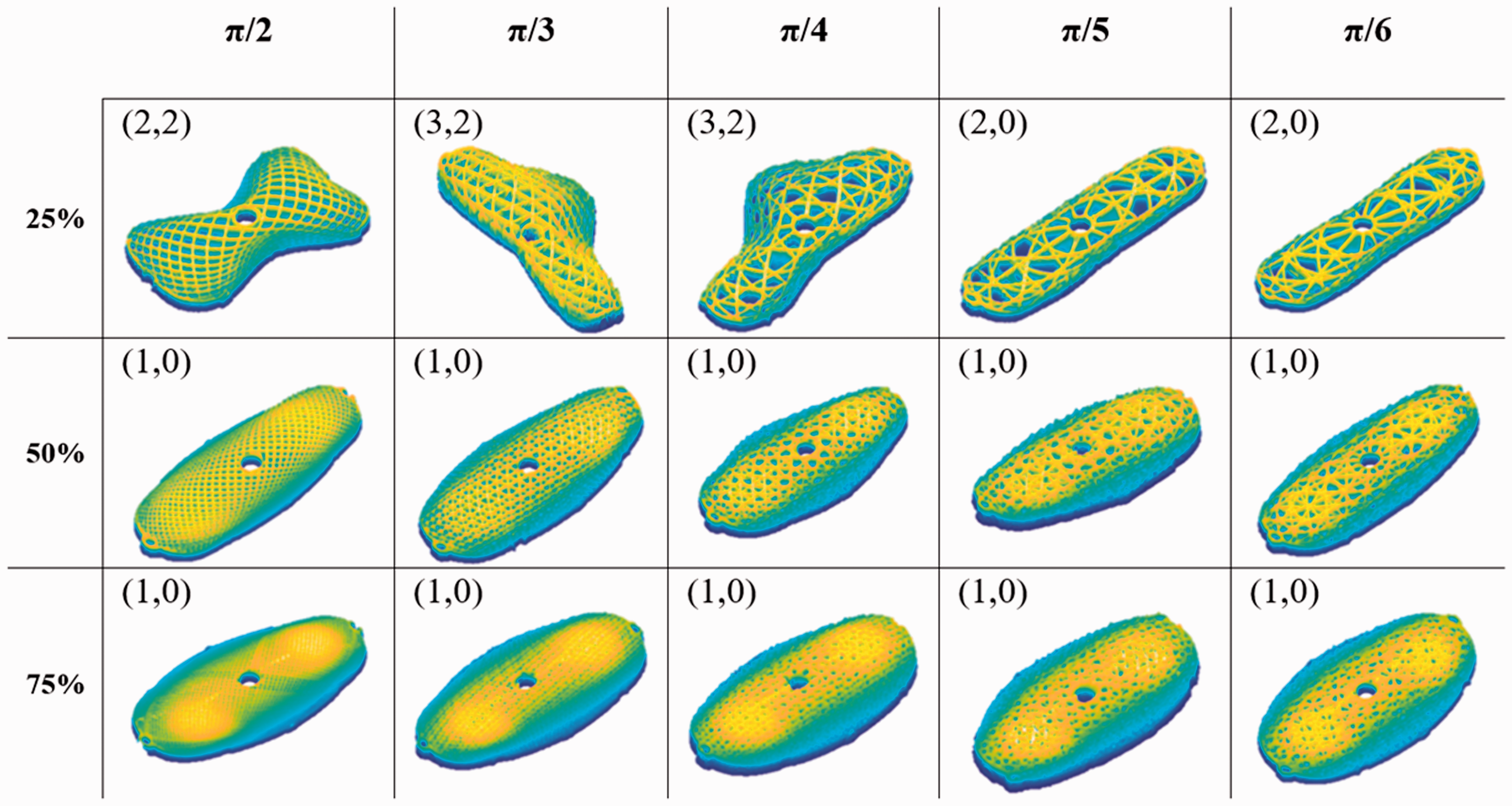
Figure 18 shows the draping modes for loading case B, with three distinct modes observed for the specimens with 25% infill. Comparing with loading case A, the draping modes for different infill patterns are generally dissimilar except for the case of π/3 specimens, where both have the (3,2) mode. All the modes for the specimens with 50% infill in loading case B are different than the ones for loading case A, while for 75% they both showed a similar draping mode of (1,0).

Figure 18.

Draping modes of specimens for loading case B.

Lastly, the draping modes of loading case C were not shown here as they all exhibit a (1,0) draping mode. As expected, the addition of the weights amplifies the number of nodes present in a draped isogrid structure as it simulates a circular specimen with a larger diameter and thus increased mass. As described in section Draping coefficient, at the 25% infill, the infill pattern and its introduction of anisotropy to the specimens is significant. The impact of this directional behavior can be observed in distinct draping modes observed in loading cases A and B for the 25% infill. At higher infill percentages, i.e., 50% and 75%, the anisotropy in the specimens diminishes and they behave more like an isotropic material. This is clearly observed with the identical draping mode of (1,0) at the 75% infill for all infill patterns and loading cases.

Conclusions

In conclusion, this study presents a novel automated draping analysis procedure to characterize the draping behavior of 3D printed flexible isogrid structures. A multi-camera ADA was designed and built that uses image processing to find specimens’ draping coefficient (DC) and draping modes. Specimens were circular in shape and 10 cm in diameter designed to accommodate up to a maximum of eight weights on their perimeters. Three loading cases were considered: (a) eight additional weights; (b) four additional weights; and (c) no additional weights. Specimens with five different infill patterns and three different infill percentages were manufactured using the ADIMLab 3D printer. For the 25% infill, the impact of the infill pattern on the DC was clear for the three loading cases. For loading case A, the π/3 specimen showed the smallest DC of 21.9%, while the maximum value was observed for the π/5 specimen. On the other hand, for loading case B, the π/5 specimen showed the smallest DC (34.1%) and π/2 specimen had the highest value (38.7%). At higher infill percentages (50% and 75%), it has been generally observed that higher order isogrids demonstrate higher DC values for the three loading cases. The highest DC was obtained for the π/6 specimen with 75% infill for all loading cases. Specimens’ mass was measured and was not the sole contributor to differences in DC values. A draping mode classification is proposed as (# of convex pleats, # of concave pleats). For the three loading cases, the maximum number of convex and convex pleats was three, resulting in a (3,3) draping mode. By determining the draping coefficients and modes of different specimens, novel design solutions can be developed for new 3D printed isogrids and garments. Different applications will determine if a high or low DC is required in addition to the constraints regarding the mass of the isogrid structures.

Future work includes testing different flexible materials within the TPE family of hyper-elastic materials. The size of the specimen and geometry can be modified to investigate the draping properties further. Lastly, the developed draping analysis software can be further improved to generate point clouds and create 3D models of the draped specimens using photogrammetry software.