
Abstract
Modeling and simulation are important tools for efficient product development. There is a growing need for collaboration, interdisciplinary simulation, and re-usability of simulation models. This usually requires simulation tools to be coupled together for co-simulation. However, the usefulness of co-simulation is often limited by poor performance and numerical instability. Achieving stability is especially hard for stiff mechanical couplings. A suitable method is to use transmission line modeling (TLM), which separates submodels using physically motivated time delays. The most established standard for tool coupling today is the Functional Mock-up Interface (FMI). Two example models in one dimension and three dimensions are used to demonstrate how the next version of FMI for co-simulation can be used in conjunction with TLM. The stability properties of TLM are also proven by numerical analysis. Results show that numerical stability can be ensured without compromising on performance. With the current FMI standard, this requires tailor-made models and custom solutions for the interpolation of input variables. Without using custom solutions, variables must be exchanged using sampled communication and extrapolation. In this case, stability properties can be improved by reducing communication step size. However, it is shown that stability cannot be achieved even when using unacceptably small communication steps. This motivates the need for the next version of FMI to include an intermediate update mode, where variables can be interchanged in between communication points. It is suggested that the FMI standard should be extended with optional callback functions for providing intermediate output variables and requesting intermediate input variables.
1. Introduction
Model-based development of cyber-physical systems is a complex task. System-level modeling typically involves submodels from a diversity of different domains and disciplines. In addition, it also requires collaboration between various organizations and teams. This is usually addressed by using co-simulation, where submodels from different simulation tools or using different solver algorithms are coupled into an overall system model. 1
The ability to connect simulation models from different tools offers several benefits. Each simulation tool is usually tailor-made for a certain problem or domain. With co-simulation, each part of a larger cyber-physical system can be modeled in its most suitable tool. In addition to providing more accurate results, this also enables multi-domain simulations and facilitates collaboration between organizations. Furthermore, distributed modeling can improve performance, modularity, and maintainability in model-based product development.
One challenge in co-simulation is to maintain numerical stability while dividing the equation system across separated solvers. 2 When using weak coupling methods, two dependent parts of a system can never be solved separately without introducing some delay to the interchanged variables. Strong coupling methods are able to avoid these delays, 3 but such methods are not supported by all tools or submodels because they require the capability of saving and restoring states. This is often difficult to implement in mature tools. If left unresolved, delayed variables can affect both stability and accuracy. Stability problems can arise from sampled communication with too low sampling frequency or from sampled communication between models with different time constants, which may result in aliasing effects. 4
Connecting simulation tools is facilitated by standardized interfaces, which reduce the need for writing custom code and using tool-dependent solutions. The most established standard for co-simulation today is the Functional Mock-up Interface (FMI). 5 In order to achieve stable co-simulation, it is important that such standards provide tools for ensuring numerical stability.
This paper analyzes FMI-based co-simulation using the transmission line modeling (TLM) technique for achieving stable tool coupling. The benefits of TLM are motivated by a numerical assessment of its stability properties. Limitations of FMI 2.0 are identified in order to motivate new features for the new FMI version 3.0.
1.1. Related work
The experiments presented in this work all use fixed communication step size. An alternative approach is to use adaptive communication step size. 6 This involves error estimation techniques and algorithms for reducing step size until the error is below a specified tolerance. When the estimated error is small, step size can be increased to improve performance. Algorithms for step size control can be either conservative or optimistic. Conservative algorithms always reject a step when the error tolerance is exceeded and repeat it with a smaller step size. Optimistic algorithms, on the contrary, allow the tolerance to be exceeded and continue with a smaller step size at the next step.
Another method is to rely on relaxation techniques, 7 which iteratively produce more accurate approximations based on an initial estimate of the resulting variables.
A drawback of both conservative step size control and relaxation techniques is that they rely on rollback mechanisms, meaning the capability of the simulation tool to undo computations and reset to a previous state. This feature is not supported by all simulation tools and is usually not possible for real-time simulations. Optimistic step size control, where the last step is not repeated when reducing the step size, does not require this. However, this may not be sufficient for sensitive models. 8
Instability can be caused by aliasing effects as a result of sampled communication patterns. Such problems are particularly likely to occur when connecting submodels with a large divergence in time constants. If this is the case, anti-aliasing filters may need to be applied.4,9 This requires submodels to provide intermediate output values, that is, not only the final value of the communication step, but also time-stamped values produced between the communication points. An anti-aliasing filter can then be applied in the master simulation tool. Although such a filter can improve stability, information that would be passed from one model to another is removed by the filter and stability and accuracy cannot be guaranteed. This method has similarities with the TLM approach in that it would benefit from similar extensions to the FMI standard that is described in this paper. Another similarity is that both methods provide good numerical stability while using fixed communication step size for data exchange. Consequently, it does not rely on rollback mechanisms and is suitable for real-time simulation.
Another method for improving performance without compromising on accuracy is suggested in Khaled et al. 10 By using context-aware extrapolation, communication step size can be increased while keeping integration errors within controlled bounds. This allows internal solvers to take longer integration steps. The technique is used in CHOPTrey, a forecasting framework for hybrid dynamic co-simulation. 11 However, this technique relies on slacked synchronization, which will always introduce some numerical errors and cannot provide guaranteed numerical stability for stiff connections.
A novel approximation technique based on dynamic decoupling and mixed-mode integration was presented in Papadopoulos and Leva. 12 Complex monolithic models are partitioned into weakly coupled submodels, suitable for distributed simulation. This allows increased simulation performance for large and complex models. Contrary to this, the work on this paper is more focused on connecting existing models from different simulation tools.
A co-simulation framework for hybrid discrete-event simulations of cyber-physical systems using FMI was presented in Camus et al. 13 Heterogeneous tools are integrated using a middle-ware based on the discrete-event system specification. In contrast to the work presented in this paper, the focus is on connecting Functional Mock-up Units (FMUs) with discrete-event components. Numerical stability problems are not investigated.
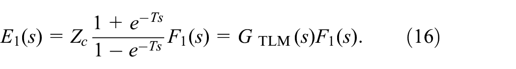
A common approach for investigating the numerical properties of a co-simulation algorithm is to discretize a test model with a coupling algorithm and then analyze the spectral radius of the resulting recurrence equation. Li 14 gives a good overview of how this method can be used to analyze numerical stability and convergence behavior of co-simulation methods. It has also been used to investigate continuous approximation techniques, 15 implicit algorithms, 3 adaptive algorithms, 16 and in the INTO CPS project. 8
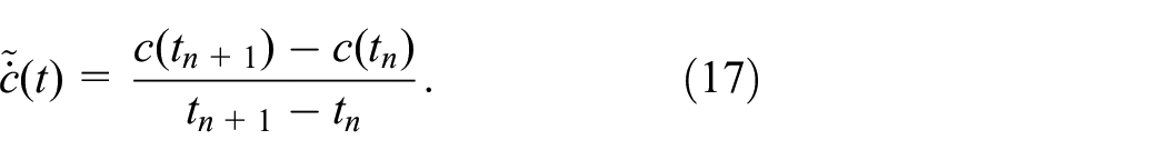
2. Background
2.1. Transmission line modeling
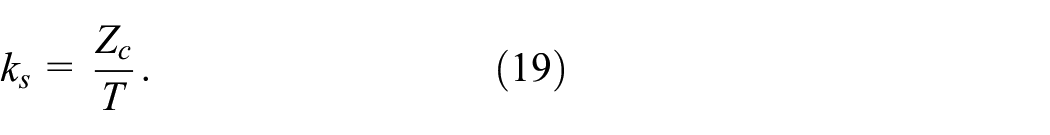
A co-simulation is a simulation of coupled simulation units. Typically, an orchestrator is used to coordinate the simulation.
17
Orchestration algorithms may be either iterative or non-iterative, use either fixed or variable communication steps, and be either sequential (Gauss-Seidel) or parallel (Jacobi). Transmission line modeling (TLM) can be seen as a non-iterative fixed-step parallel orchestration algorithm. Non-iterative co-simulation will inevitably introduce time delays to the exchanged variables. If not dealt with, such delays will affect the stability and accuracy of the simulation. TLM addresses this by exploiting physically motivated time delays for separating simulation units in time. Such delays will not affect numerical stability or accuracy because they are part of the physical model of the system. This is based on the fact that all physical interactions have a finite propagation speed. TLM originates from the method of bi-lateral delay lines
18
and provides numerically stable solver coupling.
19
Figure 1 shows an overview of a one-dimensional TLM element. All physical elements have both some inductance (
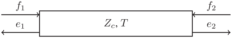
A one-dimensional TLM element with characteristic impedance
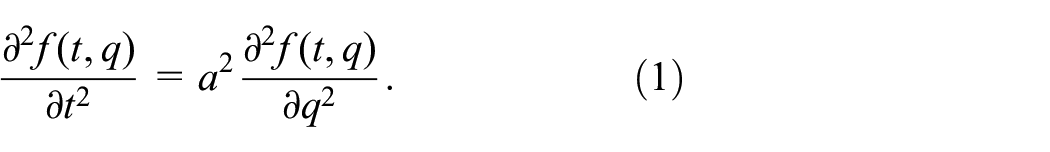
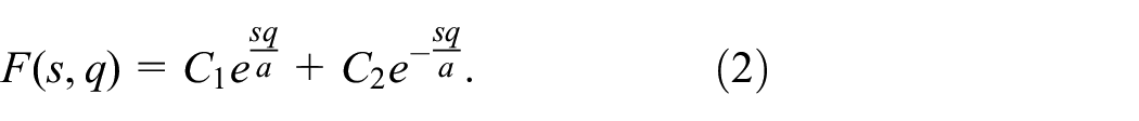
The TLM equations are derived from the plane wave solution to the wave equation (see Equation (2)):
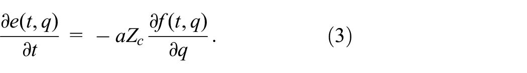
The relationship between force and effort is given by the Telegrapher’s equation:
Combining Equations (2) and (3) yields the solution for the effort variable:
Constants
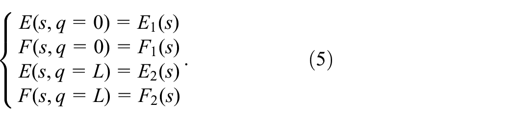
The latter two conditions also give the relationship between the variables on the two sides of the element:

Exploiting symmetry and transforming to time domain yields the governing equations:


This can be further simplified by introducing wave variables according to Equations (9) and (10), representing all delayed information from the other end of the element:


This allows the TLM equations to be written in a more compact form, as shown in Equation (12):


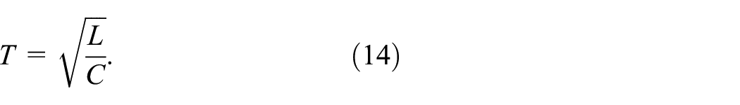
Wave variables are exchanged between the interconnected simulation models with their specified time delay. The time delay (

According to Equation (8), the effort variable on one side of the element does not depend on any variables from the other end at time
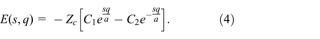
Mathematical properties of a TLM element can be analyzed by assuming zero flow on one end of the element (

The Laplace transform of Equation (15) gives the following:
TLM elements are commonly introduced by replacing ideal capacitors, for example, fluid volumes or ideal springs. Hence, Figure 2 shows the Bode diagram for
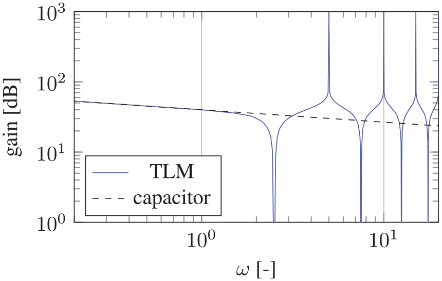
Bode diagram comparing a TLM connection with an ideal capacitor.
2.2. Functional Mock-up Interface
The FMI is an open tool-independent standard for co-simulation and model exchange. 5 Models are exchanged as compressed archives containing an XML specification file and compiled C-code. Such an archive is called an FMU. An FMU can support FMI for co-simulation (FMI CS), FMI for model exchange (FMI ME), or both. With FMI CS, the numerical solver is embedded inside the FMU. Interconnected FMUs exchange data on predefined communication points. FMI ME, on the contrary, requires a numerical solver in the tool that imports the FMU, hereafter denoted as “importing tool.” Each FMU exposes its states and their time derivatives, that is the right-hand side of the system of ordinary differential equations (ODEs). The current version of FMI is 2.0. At the time of writing, version 3.0 is still under development.
2.3. Sampling techniques
Four different sampling methods have been investigated and compared, as shown in Table 1. With FMI ME, the data flow is controlled completely by the importing tool. Thus, both inputs and outputs can be read from or written to the FMU whenever needed. This enables a continuous data exchange.
Continuity of output and input variables with four different FMI approaches.
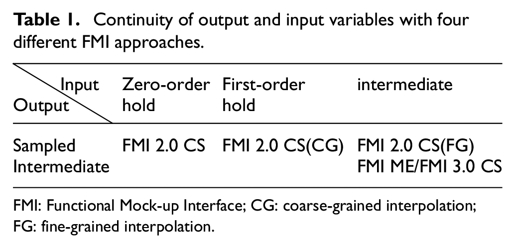
FMI: Functional Mock-up Interface; CG: coarse-grained interpolation; FG: fine-grained interpolation.
When stepping from
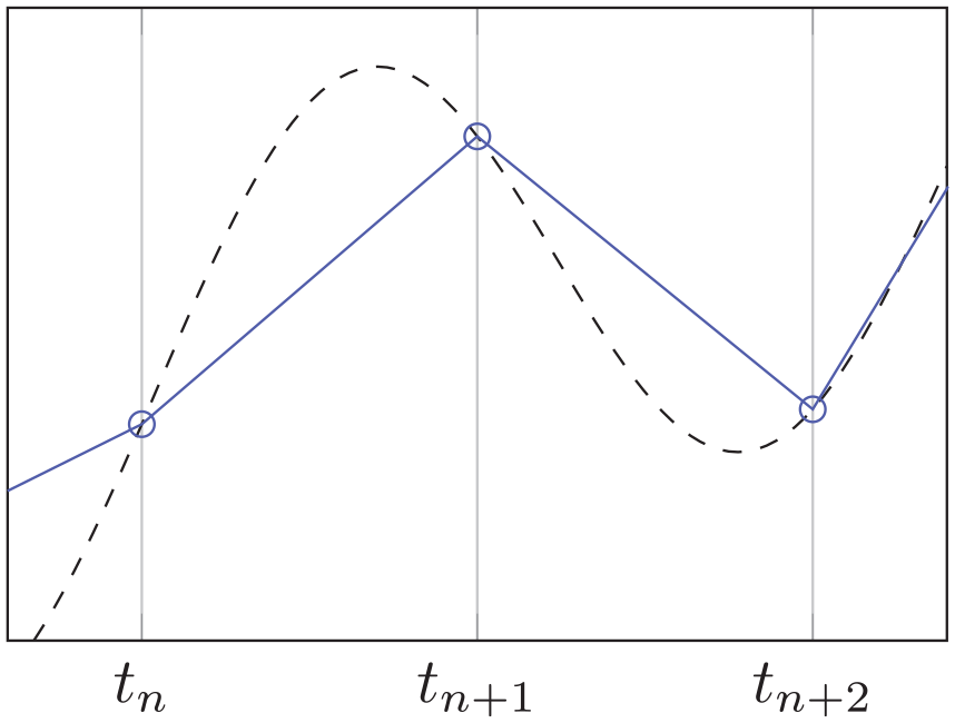
If FMI CS is used without input derivatives, inputs will be sampled according to a zero-order hold model. This often provides inadequate stability for dynamic simulations. If using TLM with zero-order hold, future information is not taken into account. Figure 3 shows the principle of zero-order hold inputs, and Figure 4 shows the communication pattern. As can be seen, both inputs and outputs are only updated before and after the communication step.
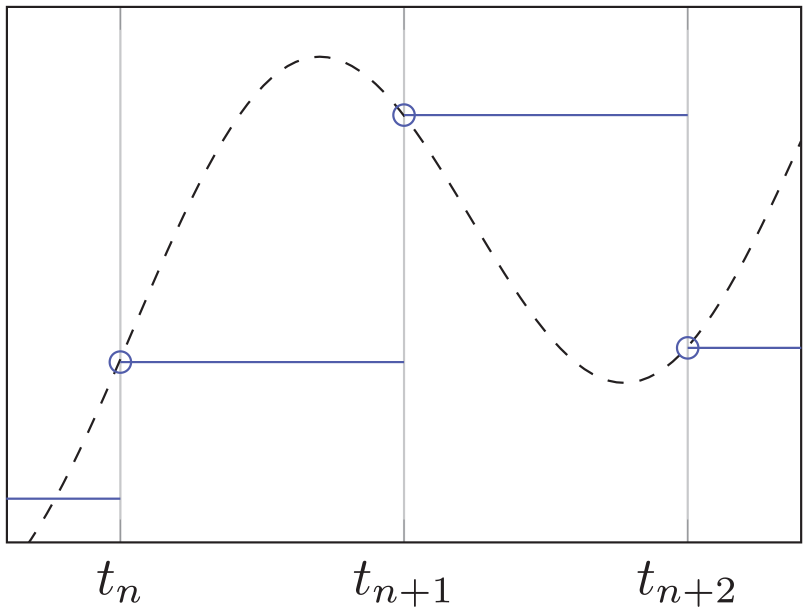
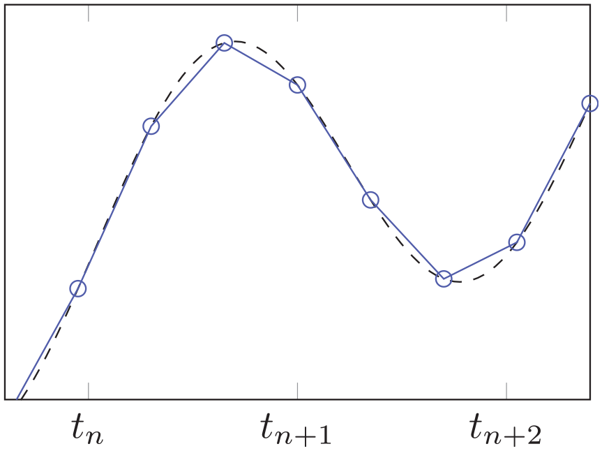
Sampling of input variables without interpolation (zero-order hold).
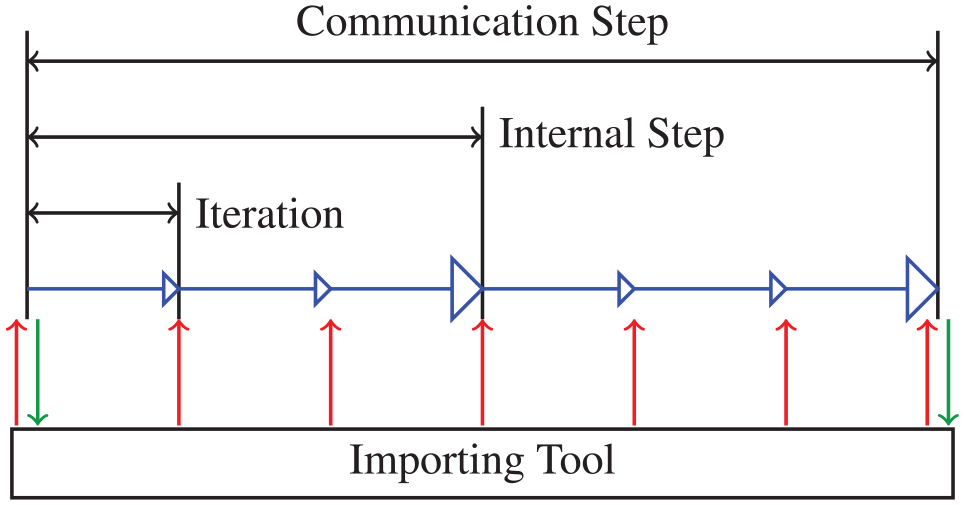
Communication pattern of FMI for co-simulation with zero-order hold. Vertical arrows represent reading inputs and writing output, respectively. Large unfilled arrows represent successful internal steps, while small unfilled arrows represent solver iterations.
In order to improve accuracy, it is possible to provide time derivatives of input variables. This method is denoted coarse-grained interpolation (CG). These derivatives can be estimated by using the difference between the values just before and just after the step:
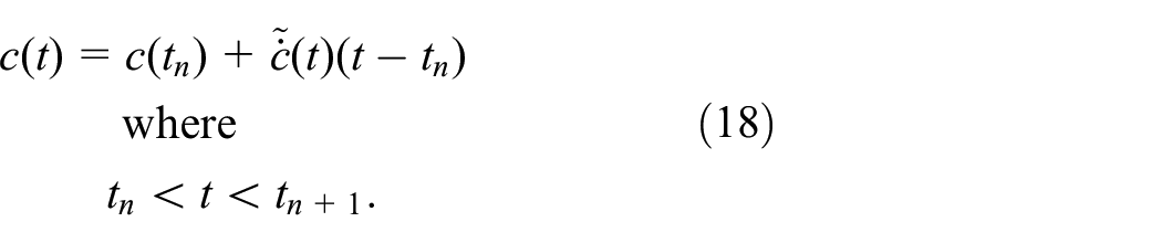
This requires that the FMU is capable of interpolating using input derivatives, which is not always the case. The first-order hold principle is shown in Figure 5, and the communication pattern is shown in Figure 6. Inputs and outputs are only updated before and after the communication step, but the input derivative is also provided. Hence, the FMU can use interpolation internally to estimate the intermediate values of the input variables.
Sampling of input variables with coarse-grained interpolation (first-order hold).
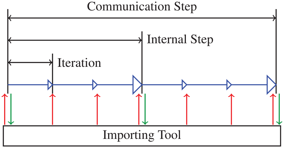
Communication pattern of FMI for co-simulation with coarse-grained interpolation. Vertical arrows represent reading inputs and writing output, respectively. Large unfilled arrows represent successful internal steps, while small unfilled arrows represent solver iterations.
Numerically stiff problems may require higher resolution of interpolation tables in order to ensure stability. This is addressed by providing the FMU with an entire interpolation table, denoted fine-grained interpolation (FG). A large number of variables and corresponding time stamps are written to the FMU using the
Sampling of input variables with fine-grained interpolation (continuous).
Communication pattern of FMI for co-simulation with fine-grained interpolation. Vertical arrows represent reading inputs and writing output, respectively. Large unfilled arrows represent successful internal steps, while small unfilled arrows represent solver iterations.
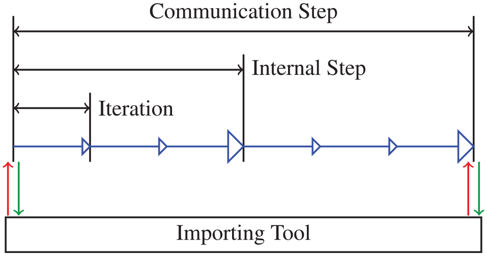
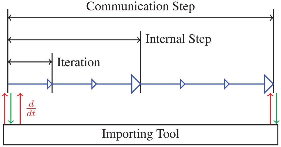
For comparison, the communication pattern when using the intermediate update mode in FMI 3.0 is shown in Figure 9. As for fine-grained interpolation, inputs can be obtained on every internal solver iteration. In addition, output values can also be sent back to the master tool after every successful internal step. Table 1 summarizes sampling techniques for input and output variables provided by each of the data transfer approaches.
Communication pattern of FMI for co-simulation using intermediate update mode. Vertical arrows represent reading inputs and writing output, respectively. Large unfilled arrows represent successful internal steps, while small unfilled arrows represent solver iterations.
2.4. OMSimulator
OMSimulator is an open-source master simulation tool for FMI-based co-simulation developed and maintained by the Open Source Modelica Consortium. 28 It supports both FMI 2.0 CS and FMI 2.0 ME, and FMUs can be connected using either causal connections or TLM. The TLM capabilities were originally developed at SKF 23 as part of the BEAST simulation tool. 29 TLM submodels communicate with the simulator using Transmission Control Protocol/Internet Protocol (TCP/IP) network sockets, which enables the use of distributed computers. OMSimulator has a C API and scripting support for Lua and Python. There are also graphical user interfaces in OpenModelica Connection Editor (OMEdit) 30 and Papyrus. 31 In addition to the demonstrator models in this paper, OMSimulator has been used for modeling cyber-physical aircraft systems. 32
Interconnected TLM FMUs may not always use the same integration step size. Integration step sizes may also vary during simulation in case an FMU is using internal step size control. OMSimulator handles this by allowing asynchronous data exchange. Whenever a step in a submodel is complete, it sends time-stamped data to the master simulation tool. These data are inserted into the interpolation table of the other FMU. Whenever input data are required by an FMU, they are interpolated from this table. This approach is enabled by the use of physically motivated delays. Assuming the maximum integration step in each FMU is limited to half the TLM delay, data will always be available for the entire duration of each macro step. Figure 10 shows the communication pattern between two FMUs.
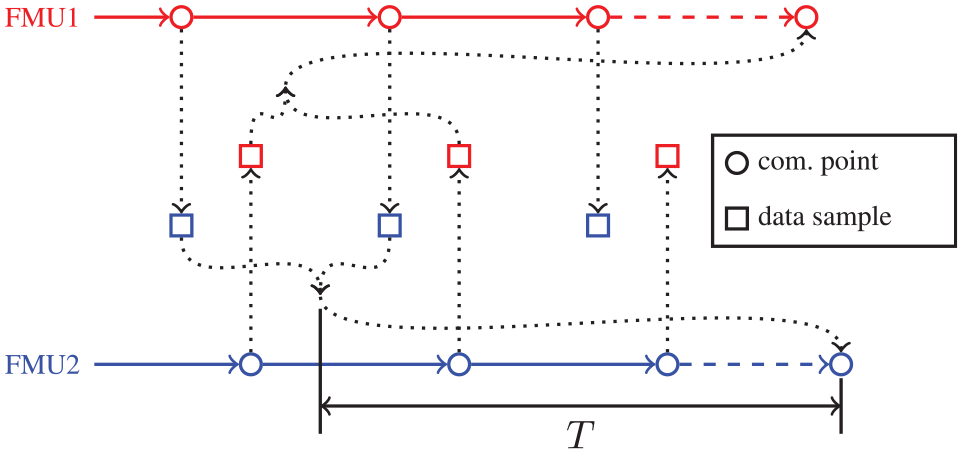
Asynchronous communication pattern with interpolation used by OMSimulator.
Choosing an interpolation method is a trade-off between accuracy and stability. Higher order interpolation may produce more accurate approximations. On the other hand, it can result in aliasing problems when connecting two models with a large deviation in time scales. While linear interpolation may be less accurate, it guarantees that the interpolated value is always between the two surrounding values, which reduces the risk of instability. One of the strengths of the TLM method is that it effectively allows both solvers to use interpolation. The same is true for strong coupling methods, but the TLM method requires no rollback. This results in a method with the same stability properties as strong coupling methods, as shown in the numerical stability analysis section, but without the performance penalty or the implementation complexity.
3. Case studies
3.1. 1D demonstrator model
A spring–mass system with three masses is used as a one-dimensional (1D) demonstrator model. A monolithic reference model is created in OpenModelica (see Figure 11). The composite model is created by replacing the leftmost spring with a TLM element (see Figure 12). Time delay and characteristic impedance are tuned so that the spring stiffness

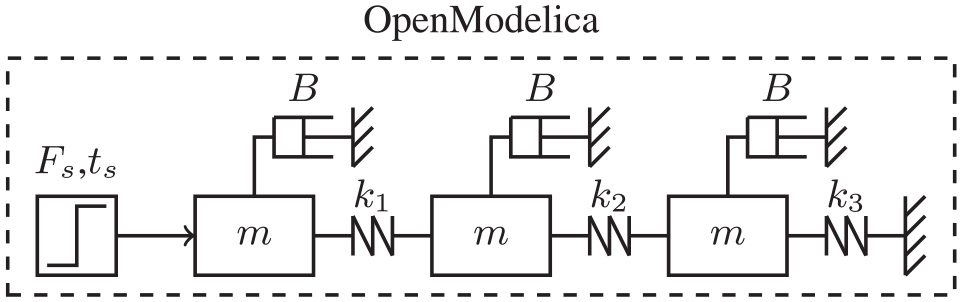
Monolithic reference model of 1D spring–mass demonstrator model.
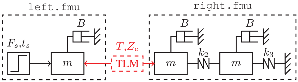
One-dimensional spring–mass demonstrator model consisting of two FMUs.
3.2. 3D demonstrator model
For analyzing the proposed methods under more realistic conditions, an industrial demonstrator for evaluation of cyber-physical systems including rolling bearings has been developed. An earlier prototype of the demonstrator was described in Braun et al. 33 The composite model represents a hydraulic crane as shown in Figure 13. Submodels include mechanical parts, a hydraulic circuit, and a controller. Figure 14 shows an overview of the interconnected submodels. The bearing is modeled in BEAST 29 and includes flexible bodies and contact mechanics. Other mechanical bodies are modeled as rigid bodies in Dymola. 34 They are subsequently exported to OMSimulator as FMUs, for either CS or ME. Finally, the hydraulic circuit and the controller are modeled in Hopsan, 35 a simulation tool for hydraulic and mechatronic systems developed at Linköping University. Hopsan is based on TLM technology and has previously been used for co-simulation.22,36
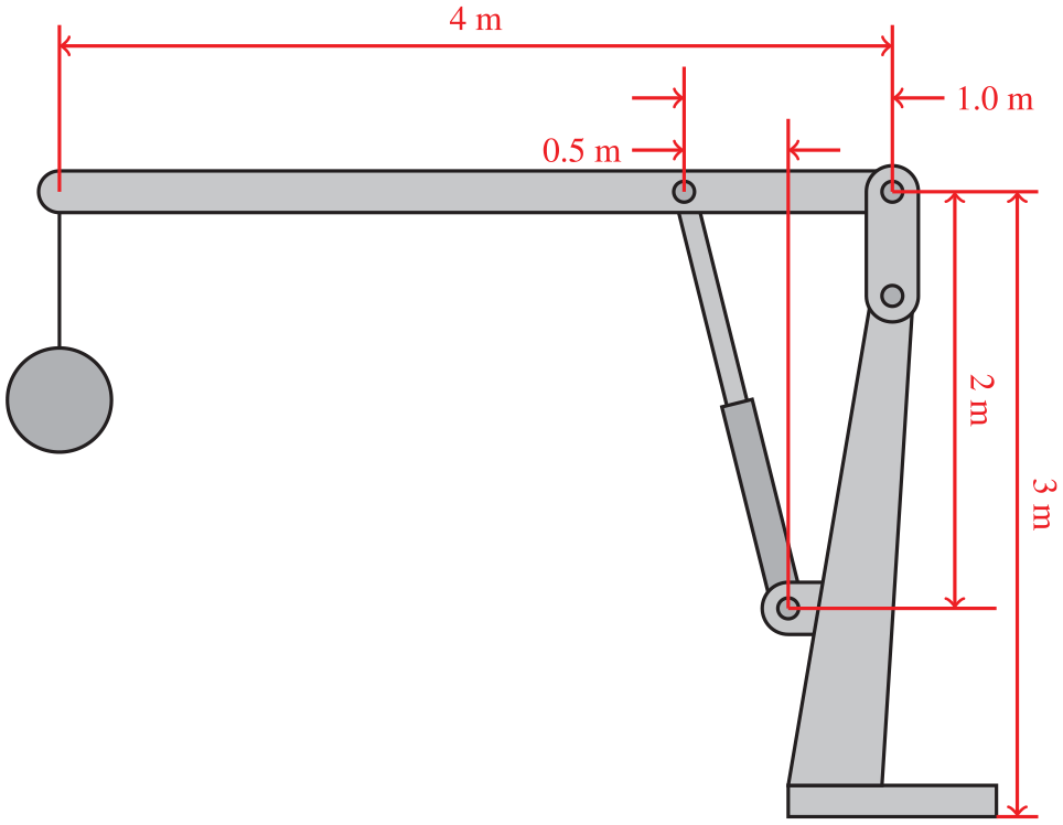
Geometry of the hydraulic crane demonstrator model.
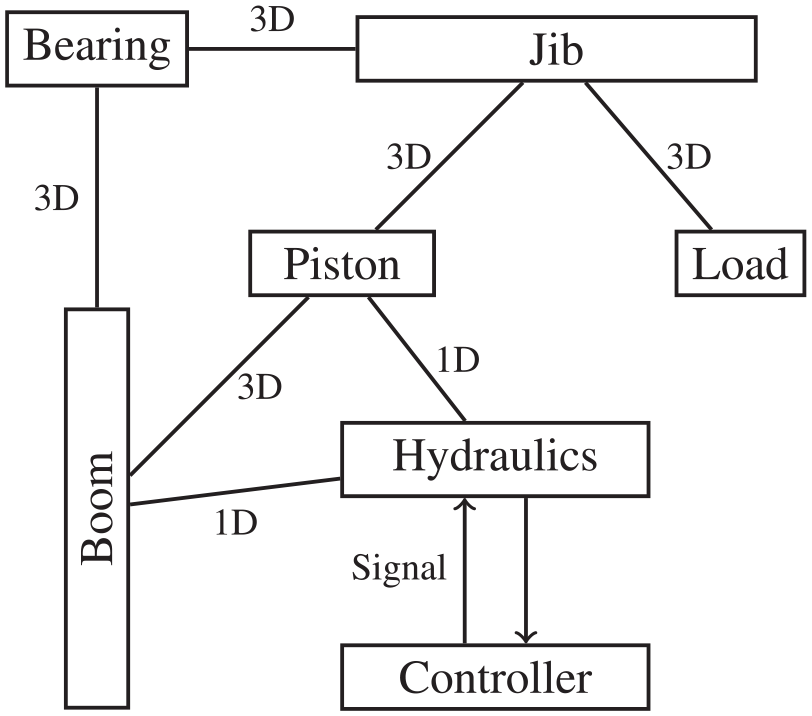
Structure of composite model and connection types with 1D and 3D TLM elements.
No single tool is capable of simulating all the parts of the crane model without simplifications. For this reason, it is not possible to create a monolithic reference model. This is the main reason why this study requires co-simulation. Consequently, FMI ME must be used as reference for the experiments with FMI CS. FMI ME provides the best possible results since it supports both intermediate outputs and intermediate inputs. All simulations on the crane model use the TLM method. Parameters for the translational and rotational connections are as follows:
4. Results
Simulation results for both demonstrator models were compared to reference simulations. For the spring–mass–damper model, a monolithic reference model was used. The crane demonstrator uses a reference simulation with FMI 2.0 for model exchange, since it cannot be converted to a monolithic model. Both reference models provide stable results.
4.1. FMI 2.0 CS (zero-order hold)
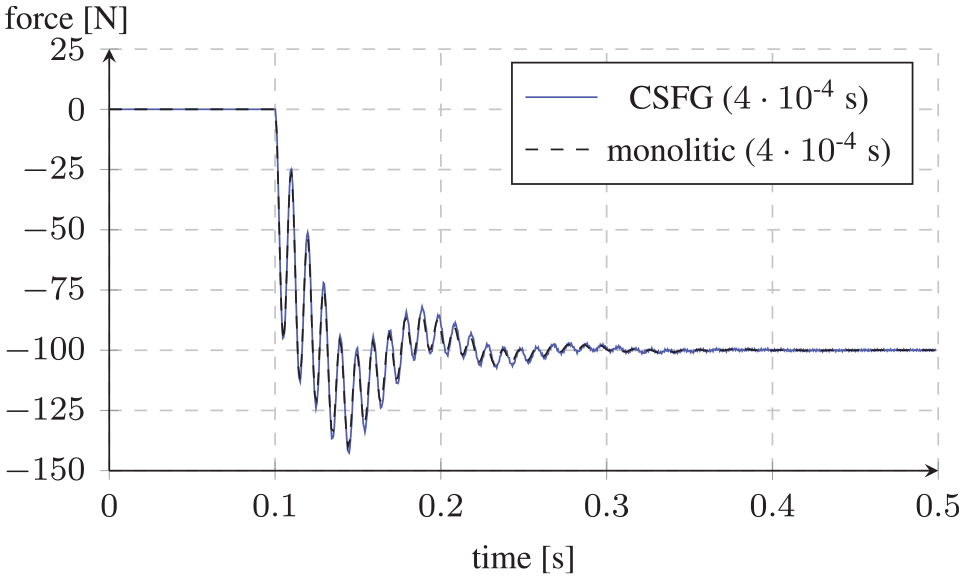
Both models were first simulated with FMI CS without providing input derivatives. This results in a zero-order hold communication pattern. Step size is reduced iteratively to improve stability. Results for the spring–mass model are shown in Figures 15–17. Stability cannot be achieved even with
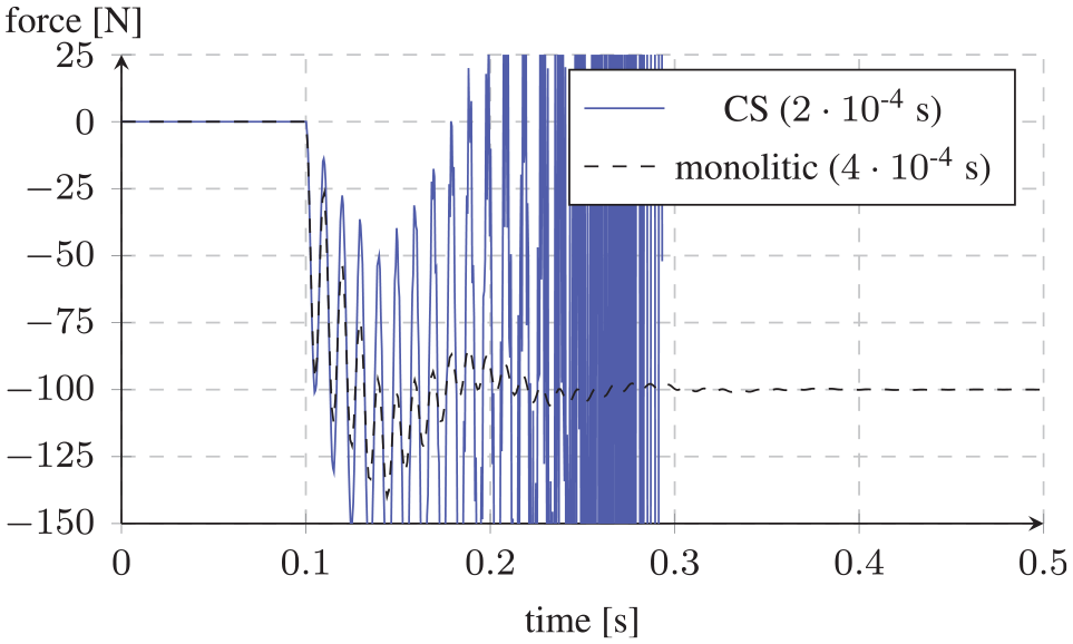
Force in 1D model with zero-order hold.
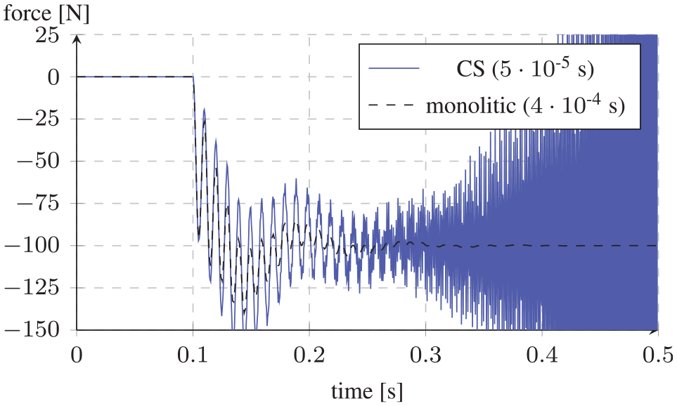
Force in 1D model with zero-order hold.
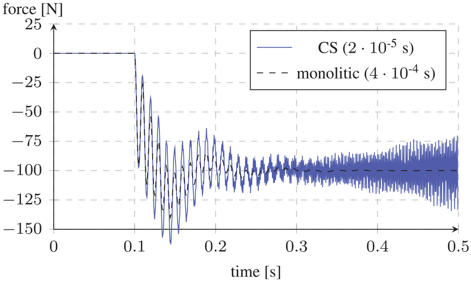
Force in 1D model with zero-order hold.
Figures 18 and 19 show results for the crane model with different step sizes. Results are similar to those for the spring–mass model. Simulation becomes unstable even when using
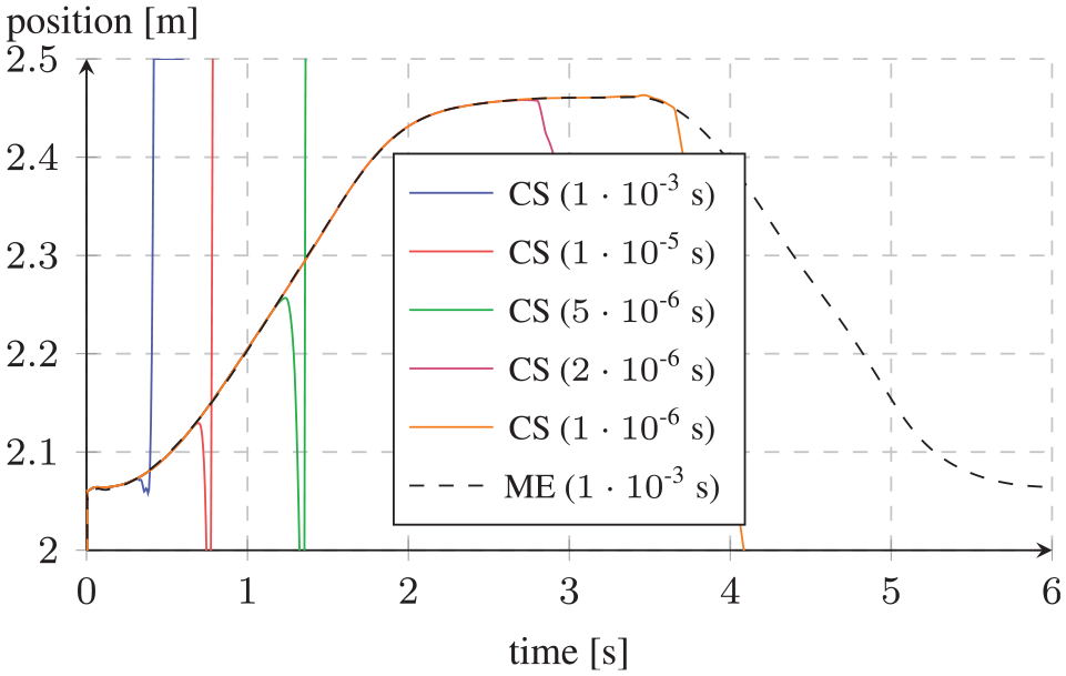
Piston position in 3D model with zero-order hold.

Motor angle in 3D model with zero-order hold.
4.2. FMI 2.0 CS (coarse-grained interpolation)
When providing FMUs with first-order time derivatives of the input variables, stability is greatly improved. Results for the spring–mass model are shown in Figures 20 and 21. When using half the step size compared to the monolithic reference model, early stages of instability can be seen. Reducing step size to
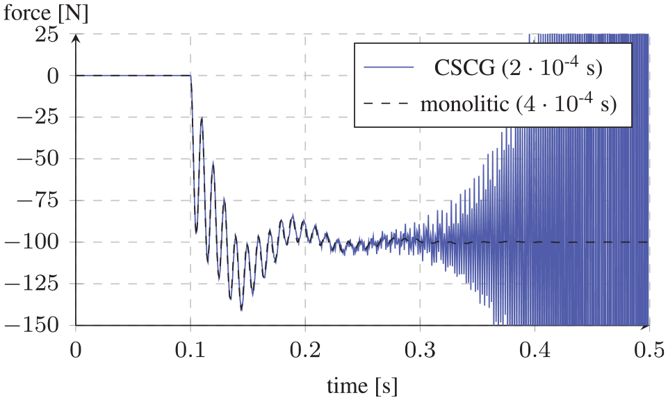
Force in 1D model with coarse-grained interpolation.
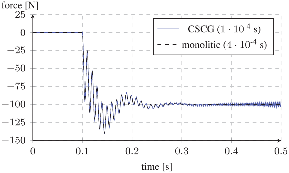
Force in 1D model with coarse-grained interpolation.
The crane model is stable for the piston motion when using the same step size as the FMI ME reference model. However, the rotational motion becomes unstable after approximately 4.5 s of simulation. Figures 22 and 23 show the results.
Piston position in 3D model with coarse-grained interpolation.
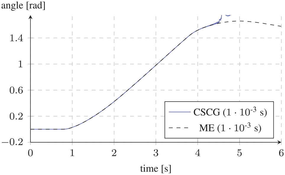
Motor angle in 3D model with coarse-grained interpolation.
4.3. FMI 2.0 CS (fine-grained interpolation)
Fine-grained interpolation was implemented by providing the FMUs with 10 evenly distributed time-stamped entries of each input variable. FMUs use linear interpolation to internally compute input variables or the time instances where they are needed. Results for the spring–mass model are shown in Figure 24. When using the same step size as the monolithic reference model, no signs of instability can be observed. It can be concluded that 10 samples are sufficient for stabilizing the connection, even though a denser interpolation table could theoretically improve stability.
Force in 1D model with fine-grained interpolation.
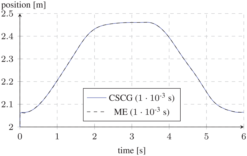
Figures 25 and 26 show the results for the crane model with fine-grained interpolation. No stability issues are observed with

Piston position in 3D model with fine-grained interpolation.
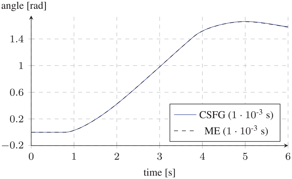
Motor angle in 3D model with fine-grained interpolation.
4.4. Numerical stability analysis
The stability properties of a coupled system can be determined by analyzing the spectral radius of the corresponding linear recurrence equation system. We will now illustrate these properties with an example model consisting of a linear two-mass oscillator as shown in Figure 27.
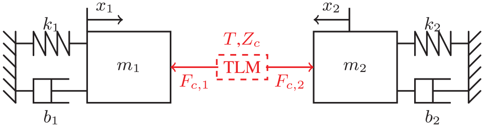
Linear two-degree-of-freedom oscillator with a TLM element.
The two submodels have position coordinates
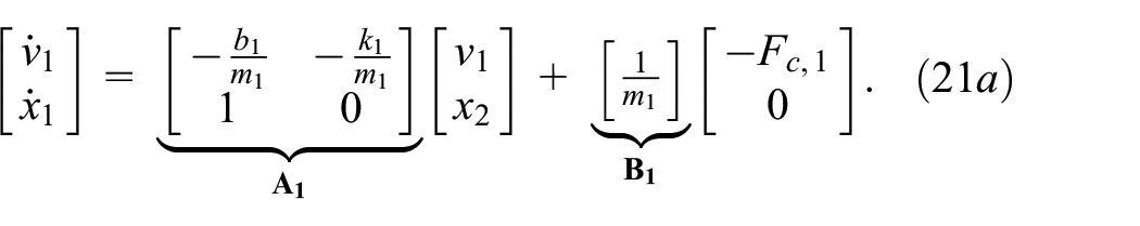
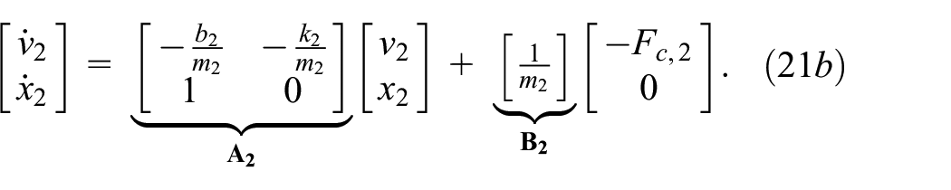
Here,

where
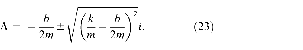
Replacing
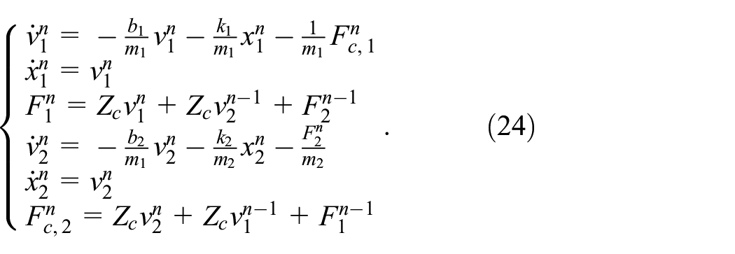
The discretization delay between points

where
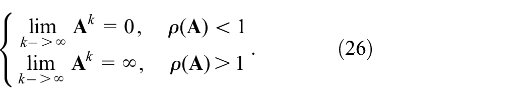
The spectral radius of matrix
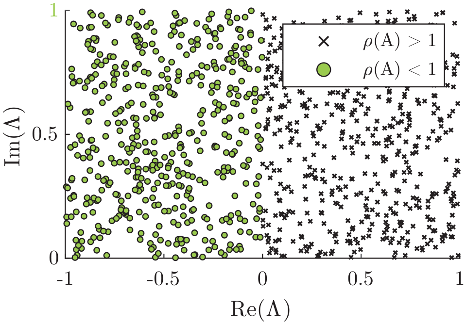
Spectral radius for the coupled system against the real and imaginary parts of the eigenvalues of the subsystems. Results confirm that TLM is A-stable.
This conforms with previous research, which has shown that when a capacitance is replaced by a TLM element, the resulting equations are equal to the trapezoid rule of integration between flow and effort.19,37 As a consequence, the stability region of a TLM coupling is the same as for the trapezoid rule.
5. TLM in FMI 3.0 CS
While the investigated interpolation techniques are shown to be effective, they require custom solutions and tailor-made FMUs. This could be avoided by allowing data transfer between the importing tool and an FMU between the regular communication points. If an FMU could request interpolated variables whenever they are needed or return variables to the master as soon as they are produced, all interpolations could be handled in the importing tool. This would enable numerically stable co-simulation with standard FMUs from an arbitrary simulation tool.
With the intermediate update mode planned for FMI 3.0, an FMU will be able to request intermediate input variables or expose intermediate outputs in between two communication points. This enables a master algorithm to run asynchronous co-simulation with TLM couplings between any FMUs, with the only requirement that each FMU supports intermediate update mode. The TLM boundary equations, for example, the calculation of effort variables, should preferably be handled by the importing tool. In this way, the only requirement on the FMUs is that they must take one effort variable as input and provide one flow variable as output. For the mechanical domain, this would equal an input force and an output speed. Such interfaces are already commonly used for, for example, force–force couplings, and many existing models can be adapted to these needs with minor efforts. This is an advantage when using co-simulation to connect existing models from different disciplines or organizations.
Fine-grained interpolation could be an alternative solution, but this requires the FMUs to handle interpolation internally. For this to be effective in the general case, it is not sufficient to rely on a fixed number of samples, as the density of the interpolation data may change between communication steps. FMI 3.0 does support array variables, but changing their length requires the FMU to enter reconfiguration mode to reallocate its memory. This would most likely reduce simulation performance significantly.
6. Conclusion
Co-simulation between different simulation tools can facilitate collaboration, improve modularity, and preserve investments. It also makes it possible to use the best suited tool for each part of a larger cyber-physical model. Efficient co-simulation requires standardized interfaces, low performance overheads, and numerically stable connections.
It is shown that FMI ME works well with TLM. FMI 2.0 for co-simulation without interpolation relies on zero-order hold sampling. With this approach, a stable connection can never be guaranteed. Stability issues arise not only due to discontinuous input variables, but also due to aliasing effects.
Coarse-grained interpolation using input derivatives provides zero-order continuity of input signals. This enables improved stability but is not able to fully stabilize the connection without reducing communication step size. While a reduction in communication step size can stabilize the connection, it also reduces simulation performance by effectively limiting the maximum integration step of the solvers in the FMUs. Moreover, it is difficult to determine in advance how small a step size that is needed to ensure stability during the entire simulation.
Fine-grained interpolation provides stable connections for both models without the need to reduce communication step size. Although output variables are sampled, the access to intermediate input variables is able to stabilize the connections. Ten samples for each communication step are sufficient in both examined models. Denser interpolation tables would provide more accurate results but are most likely only needed when connecting models with a larger deviation in time scales. A drawback with fine-grained interpolation is that a large number of variables need to be provided to the FMU at every communication step. It also requires fixed-size interpolation tables, regardless of the needs from the internal solver.
A more feasible solution would be to use intermediate variable access so that the FMU can provide intermediate output values or request intermediate input values during the step execution. Both interpolation and coupling equations can then be handled by the importing tool, which would allow connecting existing models without significant modifications. While it was shown that numerically stable asynchronous communication is possible even without the intermediate update mode, it makes the implementation significantly easier. In fact, it even eliminates the need for the communication steps, since the two solvers can exchange data whenever they need to in a truly asynchronous way.
Footnotes
Appendix 1
Funding
The author(s) disclosed receipt of the following financial support for the research, authorship, and/or publication of this article: This work has been supported by Vinnova within the ITEA OpenCPS project.