
Abstract
Digital twin is a technology that facilitates a real-time coupling of a cyber–physical system and its virtual representation. The technology is applicable to a variety of domains and facilitates more intelligent and dependable system design and operation, but it relies heavily on the existence of digital models that can be depended upon. In realistic systems, there is no single monolithic digital model of the system. Instead, the system is broken into subsystems, with models exported from different tools corresponding to each subsystem. In this paper, we focus on techniques that can be used for a black-box model, such as the ones implementing the Functional Mock-up Interface (FMI) standard, formal analysis, and verification. We propose two techniques for simulation-based reachability analysis of models. The first one is based on system dynamics, while the second one utilizes dynamic sensitivity analysis to improve the quality of the results. Our techniques employ simulations to obtain the model’s sensitivity with respect to the initial state (or model’s Lipschitz constant) which is then used to compute reachable states of the system. The approaches also provide probabilistic guarantees on the accuracy of the computed reachable sets that are based on simulations. Each technique requires different levels of information about the black-box system, allowing the readers to select the best technique according to the capabilities of the models. The validation experiments have demonstrated that our proposed algorithms compute accurate reachable sets of stable and unstable linear systems. The approach based on dynamic sensitivity provides an accurate and, with respect to system dimensions, more scalable approach, while the sampling-based method allows a flexible trade-off between accuracy and runtime cost. The validation results also show that our approaches are promising even when applied to nonlinear systems, especially, when applied to larger and more complex systems. The reproducibility package with code and data can be found at https://github.com/twright/FMI-Reachability-Reproducibility.
Keywords
1. Introduction
Digital twins (DTs) are an emerging technology that makes it possible to monitor, optimize, and control cyber–physical assets using their virtual representation (kept as a mirror of reality) in real-time. 1 They provide critical services such as state estimation, visualization, what-if analysis, anomaly detection, and self-adaptation.
Because DT services rely heavily on the existence of models of the cyber–physical systems2,3 (CPS), the dependability of the DT is a direct consequence of how much we can depend upon the models’ simulation. For example, prior to adapting the controller of the CPS, the DT needs to find the optimal and safe configuration by, for example, running simulations with alternative configurations on future predicted scenarios, while checking that safety properties are satisfied. If there is uncertainty in the model parameters, as there often is in continuous and hybrid system models whose parameters are identified from sensor data, then we may be interested in computing bounds that enclose all simulation results, based on the possible parameter values, in a technique called reachability analysis. An introduction and survey of the topic of reachability analysis are provided in the study by Althoff et al. 4 and an example application for DTs is presented in the study by Wright et al. 5
To compute reachable states of the system generally requires knowing a model of the system, which for CPSs can be hard to obtain or even unavailable because of the myriad of modeling and simulation tools used in engineering practice. Fortunately, the industry has formulated standards that make it possible to represent and integrate black box, IP-protected models. One such standard is the Functional Mock-up Interface (FMI), 6 which is currently supported by more than 150 tools. Because of these reasons, in this paper, we focus on a class of reachability analysis techniques that are data-driven (i.e. they rely on data generated from simulations), which can be applied to black-box models. Although several data-driven reachability analysis approaches have been proposed in the literature, they either do not provide probabilistic guarantees on the completeness of the exploration, or discuss handle coupled models.
1.1. Contribution
In this paper, we build upon our previous work 7 and propose a new method for computing reachable states of black-box coupled models. This reachability analysis method leverages advanced FMI standard functionality for retrieving partial derivatives of Functional Mock-up Unit (FMU) variables and numerical differential system solvers to solve dynamic sensitivity equations, which describe system sensitivity to changes in their initial conditions. The computed maximum sensitivity provides a scaling factor, which together with a nominal initial state space trajectory is used to compute approximate reachable sets.
In summary, the novel contributions of this paper are: (1) a dynamic sensitivity-based reachability analysis method of black-box models and (2) a method for composing dynamic sensitivity equation systems from coupled models implementing the FMI standard. The paper evaluates the new approach against our previously introduced data-driven method 7 by comparing reachable sets computed for linear and nonlinear dynamical systems. We also validate our approaches against a leading model-based reachability analysis tool—Flow*. 8
The paper is structured as follows. The following “Related work” section discusses related work and positions our reachability analysis approach. After that, our paper describes the preliminaries and the problem statement of the paper. The main contributions of the paper are presented in the “Reachability algorithms” section in which we formally describe our proposed reachability analysis and dynamic sensitivity equation composition algorithms. The “Validation experiments” section describes results obtained from comparing and validating algorithms, as well as discusses limitations and recommendations of the proposed methods. In the final section, we summarize our findings and propose directions for future work.
2. Related work
This paper extends our previous work, 7 where we proposed a data-driven method for computing the reachable states of black-box models with probabilistic accuracy guarantees, given a sufficient number of samples is used. This reachability method was based on estimating a maximum Lipschitz constant by simulating a model from independent and identically distributed (i.i.d.) initial conditions and their perturbations. However, for higher-dimension and more complex systems, the method requires a large number of samples to over-approximate accurately the reachable sets.
Over the years, the problem of computing the set of reachable sets of a given system has received considerable attention. In this section, we attempt to summarize this work and conclude with an argument for the novelty of the current manuscript. There are two main methods for reachability analysis: model-based and data-driven. Model-based reachability analysis uses a mathematical model of the system to compute reachable states from a given set of possible initial states. Over the years, several reachability tools have been developed, such as SpaceEx, 9 JuliaReach, 10 XSpeed, 11 and Flow*, 8 to name a few. The reachability methods have been widely used in applications that range from formal system verification to their synthesis. 4 Reachability analysis is also at the core of abstraction-based techniques for controller synthesis in both deterministic systems12,13 and stochastic models.14,15
We will focus on data-driven reachability analysis techniques, which have also been proposed for scenarios when a model of the system is unavailable or too complex, and we will use the following axes to compare and position related papers, as summarized in Table 1.
Positioning of the state of the art.
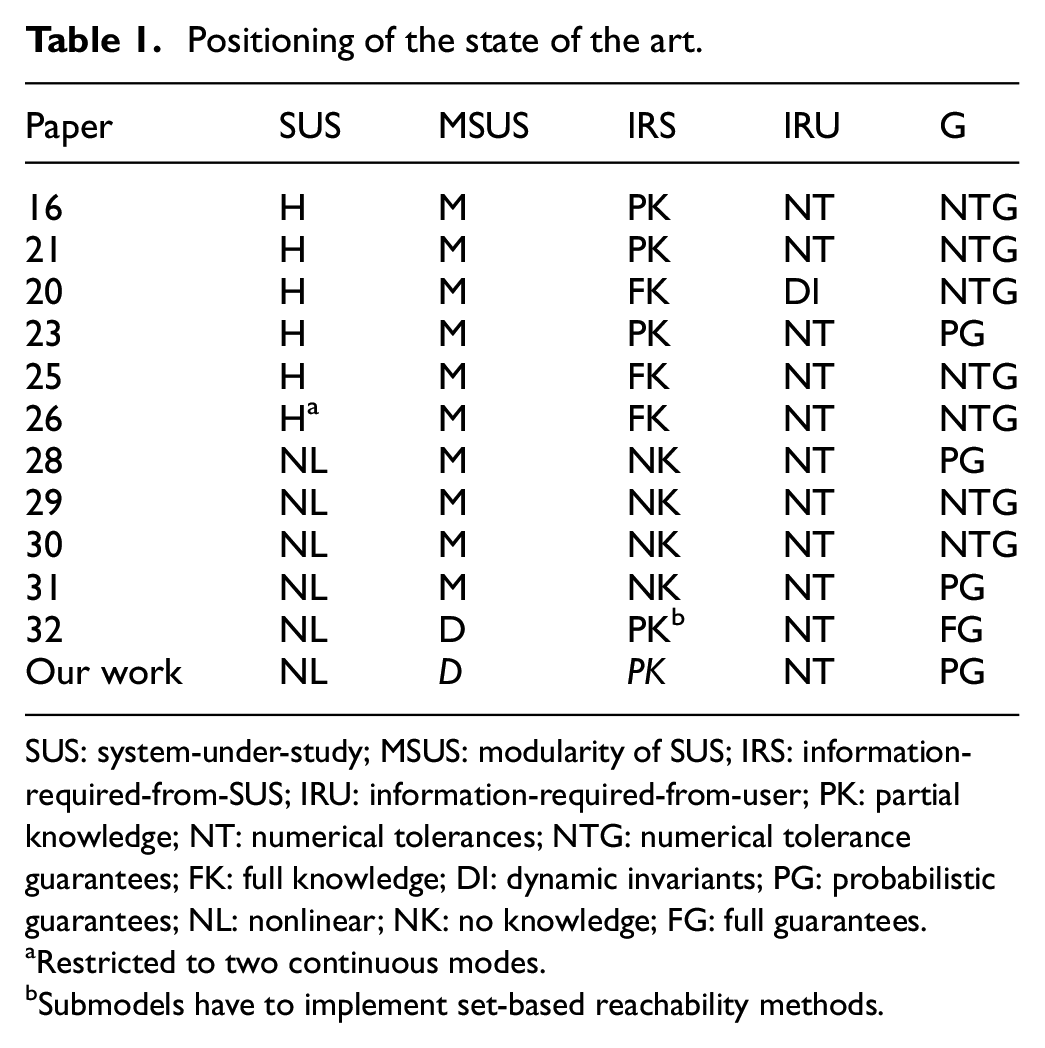
SUS: system-under-study; MSUS: modularity of SUS; IRS: information-required-from-SUS; IRU: information-required-from-user; PK: partial knowledge; NT: numerical tolerances; NTG: numerical tolerance guarantees; FK: full knowledge; DI: dynamic invariants; PG: probabilistic guarantees; NL: nonlinear; NK: no knowledge; FG: full guarantees.
Restricted to two continuous modes.
Submodels have to implement set-based reachability methods.
System-under-study (SUS): Denotes the kind of system supported by the technique. Systems can be linear/affine (L, the two are equivalent since one can transform an affine system into a linear one through extension of the states); nonlinear (NL, the type of Equation (1)); hybrid linear (HL, systems with different modes but within each mode the dynamics are linear); and hybrid (H, as in the most general hybrid automata). Within the hybrid category, there are kinds of systems, but we abstain from discerning those.
Modularity of SUS (MSUS): Represents the degree of support for decoupled SUS. The categories are monolithic (M) and decoupled (D). For example, systems that are represented by communicating sub-models, like the one presented in Figure 1, are decoupled.
Information-required-from-SUS (IRS): Denotes the degree of information that the technique requires from the SUS. Possible categories are full knowledge (FK) of the systems equations; partial knowledge (PK), where for example, the Jacobian of the system can be queried through an API, without the knowledge of the equations; and no knowledge (NK), where the model can be simulated through an API, without any knowledge of the equations.
Information-required-from-User (IRU): Denotes the kind of information the user needs to specify. At the very least, we have information on numerical tolerances (NT), and on the opposite side, we have information on dynamic invariants (DI).
Guarantees (G): Denotes the level of guarantees offered by the technique. We can have reachability up to numerical tolerance (NTG), probabilistic guarantees (PG), and guarantees including numerical approximations, that is, full guarantees (FG).
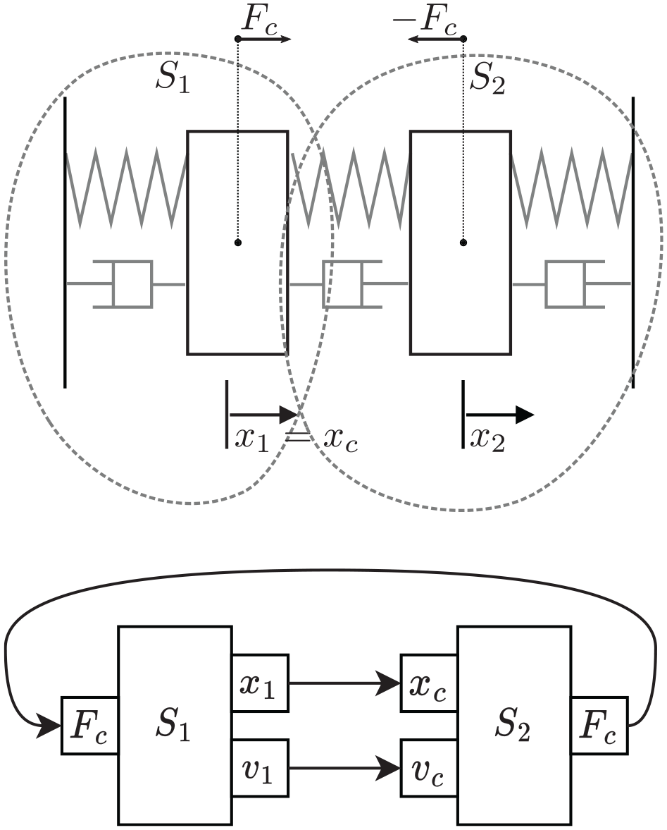
Example double mass-spring-damper system.
2.1. Dynamic sensitivity-based reachability analysis
We begin with the works that are based on solving or estimating the solution to the dynamic sensitivity equations, and then using their solution to build the reachable set, as introduced in Background and Problem Statement. Among these, we highlight the methods described in the study by Donzé and Maler,
16
where a notion of expansion function is introduced, which can be seen as the application of the dynamic sensitivity to a given disturbance in the initial condition (cf. Theorems 3 and 4 in the study by Donzé and Maler
16
). The benefit of this method is that more simulations can be run, and in fact, thanks to the dynamic sensitivity information, the initial conditions can be iteratively tried in a way that attempts to drive the system into an unsafe state (to quickly falsify a safety property). In the same way, more samples can be taken, if more accuracy is needed. In the same paper, the technique was extended to hybrid systems without reset actions (but reset actions could be included, provided they are differentiable with respect to their inputs). The extension requires that the dynamic sensitivity of the jump time be computed as part of the system, and uses results developed earlier in, for example, the study by Hiskens and Pai.
17
Later, Geng and Hiskens
18
revisits the jump conditions required to apply second-order sensitivity analysis to hybrid systems (second-order sensitivity analysis permits an approximation of the flow around a nominal trajectory that will have an error in the order of
Another similar approach to sensitivity-based reachability analysis is proposed in C2E2, 20 which originally was designed for continuous and switched systems and, in the later paper, 21 extended to handle hybrid systems as well. Their work proposes a generic “discrepancy function,” which provides a time-varying maximum distance bound on any two trajectories originating from the initial set. As far as we could assess, the notions of a discrepancy function and an expansion function are closely related, with both capable of being generated from the dynamic sensitivity equations of the system, or over-approximations of it. The reader can see various methods for computing discrepancy functions for different classes of models in the study by Fan and Mitra, 22 and the DryVR tool 23 expresses the problem of finding a discrepancy function as a problem of learning a linear separator. The tool also provides a probabilistic accuracy guarantee on the computed discrepancy function, given a sampling complexity formula is followed.
HS3V24,25 is a similar tool, which uses sampling and a Lipschitz-based discrepancy function to estimate reachable sets. Their approach also introduces a method called dynamic simulations-spawning (s-spawning) to bound error growth and adds new simulations to deal with discrete jumps. It is worth mentioning a few other simulation-based approaches26,27 that provide methods to compute a time-varying function that provides a distance bound on trajectories between the system and a simpler counterpart. The simulations of the simpler model can be combined with the time-varying function to yield reachable sets.
2.1.1. Optimization-based reachability analysis
The paper by Xue et al. 28 uses samples obtained from simulating a black-box model to learn an underlying model by solving a robust optimization problem, which provides probabilistic model accuracy guarantees. Different template models can be used for learning the black-box model (e.g. polynomial functions). A similar approach is presented in work 29 where the author’s approach uses sampled noisy data to identify a set of models, which are then over-approximated with zonotopes.
The paper 30 presented a sampling-based reachability analysis approach that is based on random set theory and adversarial sampling. The main novelty of the work is utilizing recent advances in deep learning to iteratively discover trajectories that help to converge the actual reachable set. In other learning-based reachability analysis work, the NeuReach tool 31 was introduced that efficiently computes reachable sets and provides a probabilistic accuracy guarantee.
While learning-based methods can improve the performance of the reachability analysis, the main drawback is that the underlying deep learning model has to be retrained for different systems.
2.1.2. Decoupled reachability analysis
Finally, we highlight the work by Coënt et al., 32 which acknowledges the need for reachability analysis techniques that work in parallel for de-coupled models, such as those commonly found in co-simulation scenarios. 33 In the aforementioned paper, the authors introduce an interval-based reachability method, which uses set-valued Runge–Kutta integration methods. 34 The reachability computation is done step-by-step, advancing time after the reachable set of each step has been computed. At each step, each sub-model is a black-box simulation that computes the interval of outputs based on the interval of inputs. All sub-models’ intervals are then exchanged and the step is repeated until a fixed point is reached. A method for ensuring the robust stability of FMI co-simulation models has been presented in paper. 35
2.2. Novelty of contribution
As summarized in Table 1, compared to the state of the art, the novelty of our contribution is in providing probabilistic guarantees for decoupled black-box models.
3. Background and problem statement
3.1. Continuous time systems
We consider continuous-time systems, characterized by a tuple

which, thanks to the local Lipschitz assumption, always has a unique solution, regardless of the initial condition.
In order to represent the solution of Equation (1) as a function of time

with
3.2. Reachability analysis
Reachability analysis is a technique for computing the set of all reachable states of the solution to Equation (1) for each possible initial condition from a set

To capture all reachable states, starting from the initial time up to a given simulation time
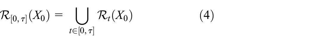
Reachability methods provide a powerful approach to verifying safety requirements of dynamical systems under uncertainty, 4 and are supported in a range of tools such as SpaceEx, 9 Checkmate, 36 and Flow*. 8 Furthermore, to efficiently and accurately over-approximate reachable sets, different convex and nonconvex set representations have been developed. We refer the reader to the aforementioned works for more details on how to over-approximate the reachable set in Equation (4).
3.3. Co-simulation and the FMI standard
Co-simulation is a technique where multiple black-box simulators are coupled together (see the studies by Gomes et al. 33 and Fitzgerald et al. 37 for introductions to the topic). The difference between a black-box simulator and a black-box model is that the simulator contains the sub-model and approximates its numerical solution, given an input signal. Since simulators are coupled in feedback loops, the coupled solution is computed iteratively, moving forward in time and approximating the solution at each new time point from the solution at previous time steps. The FMI standard 38 establishes the interface of the black-box simulators, also called FMUs, in the nomenclature of the standard. An individual FMU is comprised of a description file (in XML), which declares visible-state variables and other model information, and binaries that implement the application programming interface to interact with the FMU. Over the years, a number of well-known modeling and simulation tools have been upgraded (e.g. Simulink, 39 OpenModelica 40 ) or developed (INTO-CPS tool 41 ) to support FMI standard.
The mandatory interface functions, implemented by an FMU denoted as
A co-simulation scenario is a set of FMUs and a description of how they are connected. It is often depicted in a diagrammatic form, as Example 1 shows.
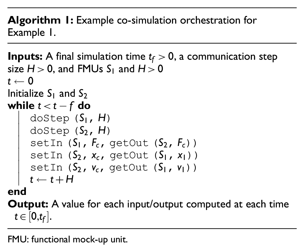
FMU: functional mock-up unit.
In addition to the mandatory functions each FMU implements, the FMI also adds a number of optional functions, that can be optionally implemented by FMU exporting tools. From these, we highlight the functions that allow one to compute partial derivatives. Neglecting efficiency issues, we denote this function as
3.4. Problem statement
In this paper, we address the problem of computing reachable states of DT virtual models as formally defined in Problem 1.
In the above problem statement, we assume that a black-box model of the system
3.5. Dynamic sensitivity equations
We define the dynamic sensitivity equations, also called the variational equations or just sensitivity equations, of the system in Equation (1) as the different derivatives of the
For a system with
Given state variables
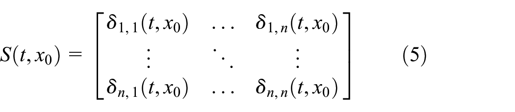
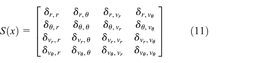
The dynamic sensitivity is a matrix represented as follows:
The dynamic sensitivity equations shown next represent an extension of Equation (1) with differential equations that relate
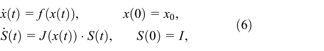
where we have omitted the dependency to
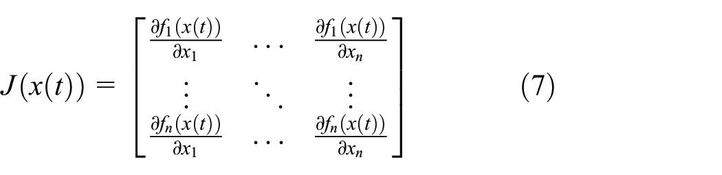
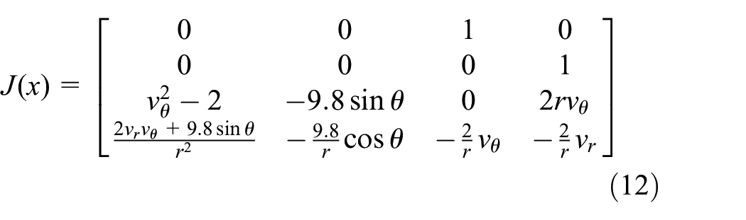
represents the Jacobian matrix of the continuous-time system and
To derive Equation (6), we differentiate
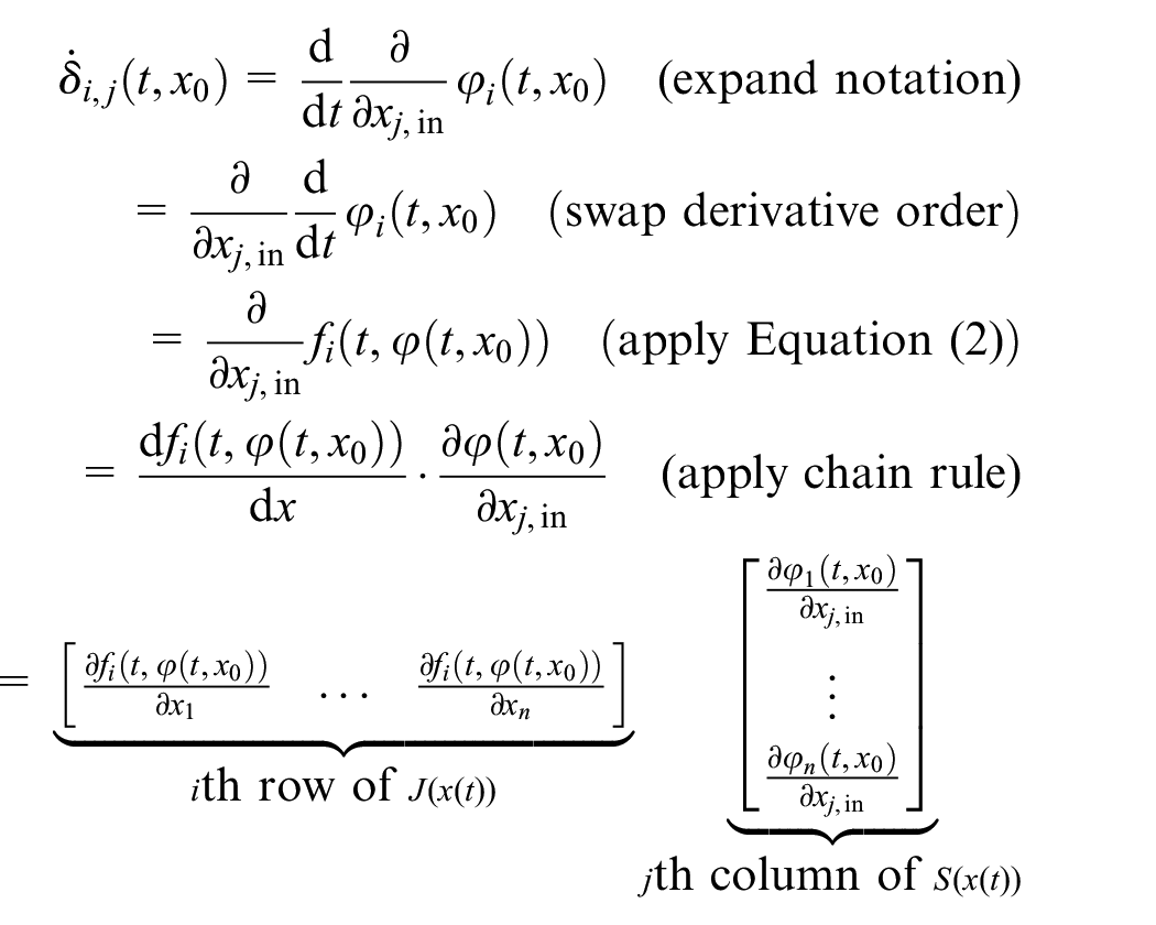
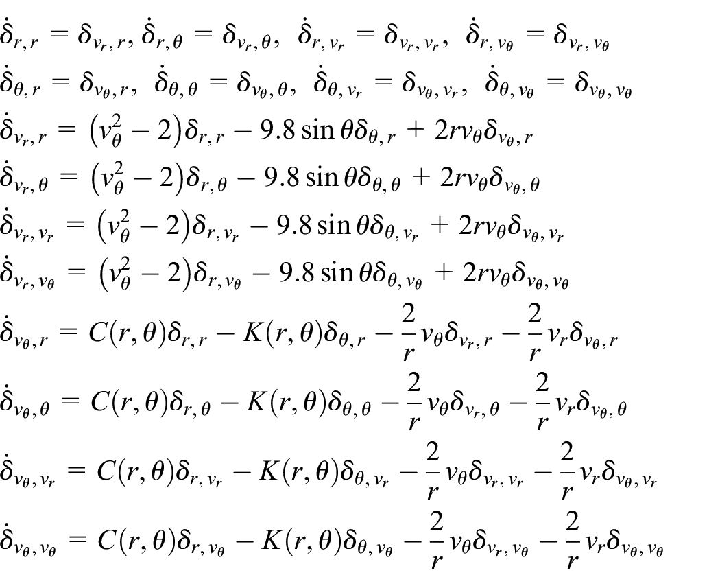
Taking all entries of
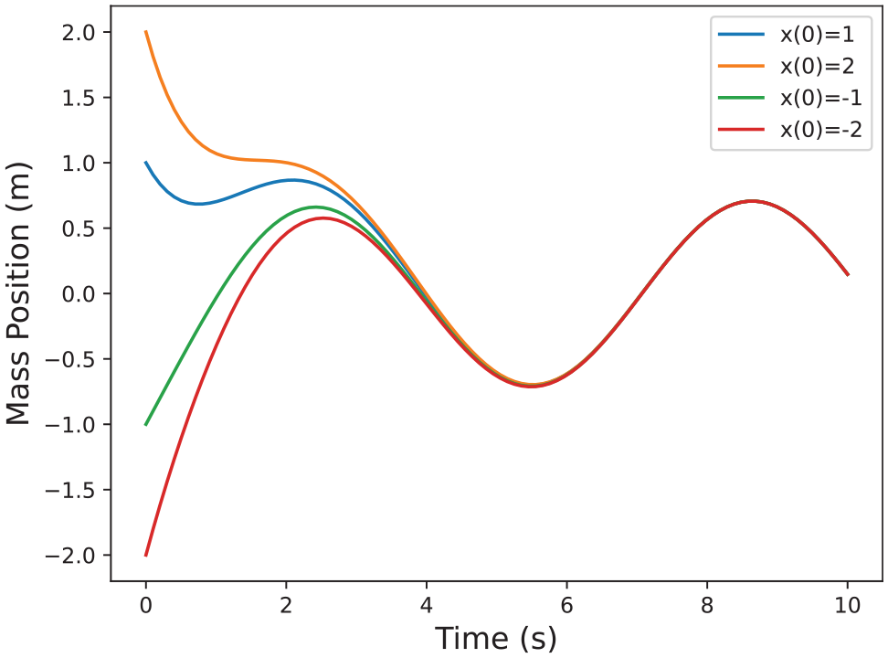
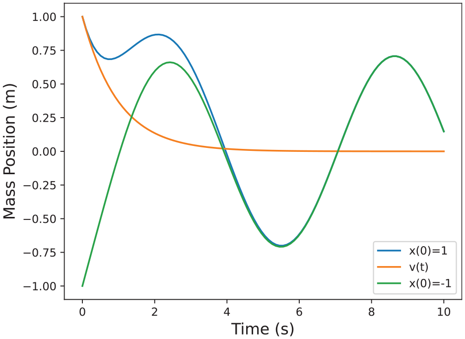
Example solutions for the system in Example 2.
Applying Equation (6), the expanded system is as follows:
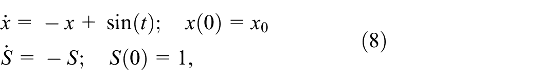
with solution:
plotted in Figure 3.
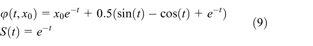
Example solutions for the system in Example 2 including the sensitivity.
The sensitivity matrix is therefore as follows:
As we show next, the Jacobian,
As we have seen before we can get the expression of
where:

3.6. Interpretation of sensitivity equations
We demonstrate here how dynamic sensitivity equations can be used to approximate the reachable set
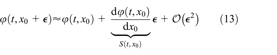
where the
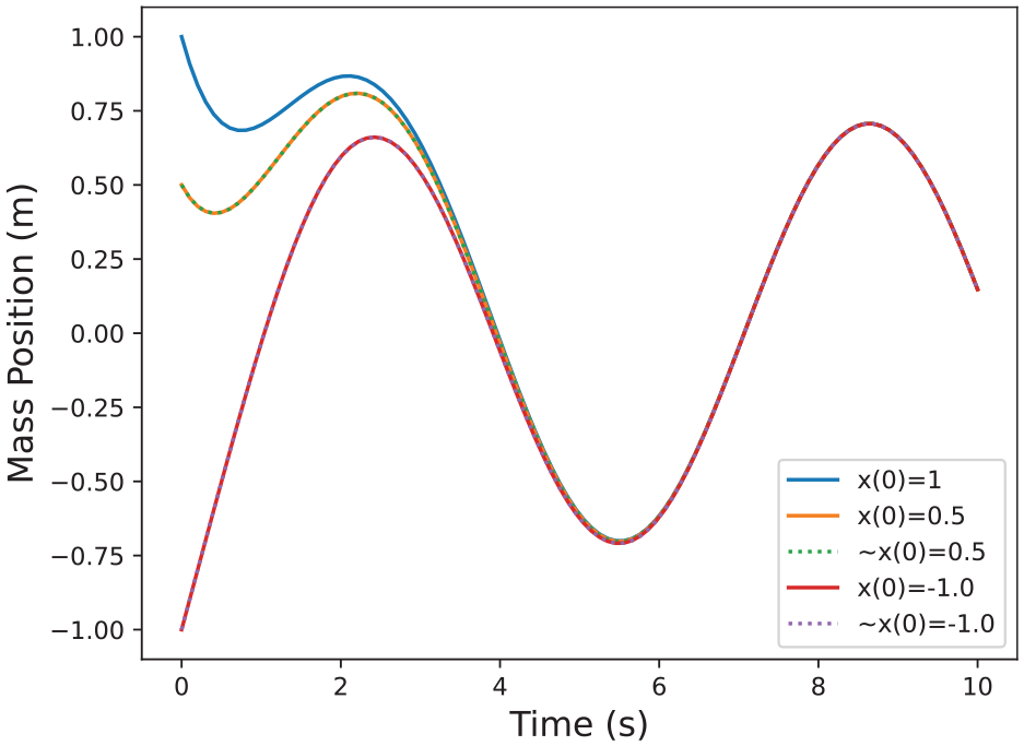
Example estimated solutions for the system in Example 2 around nominal trajectory
To summarize, for an expanded dynamic sensitivity system as in Equation (6), and a given initial set
Discretize
For each
Because of continuity, any set of states between a trajectory and the estimated trajectories in its vicinity are reachable, so we can form flow pipes uniting the nominal trajectory and all trajectories of interest in its vicinity.
The above approach does not necessarily generate over-approximations of the reach set for nonlinear systems since the higher-order terms in the Taylor expansion are eliminated without appropriate quantification of the induced error. In the following sections, we provide two techniques that are based on random trajectories of the system and provide probabilistic correctness guarantees.
3.7. Robust convex programs
This section provides the mathematical details for robust convex programs (RCPs) and data-driven approximations of their solution. The content of this section is provided in its full generality. We will utilize Theorem 1 and Theorem 2 presented in the sequel to establish the correctness of our data-driven framework. The reader can refer to the papers43,44 for the full exposition of the results presented in this section.
Let
An example of the
Let
An example of the
where

with confidence
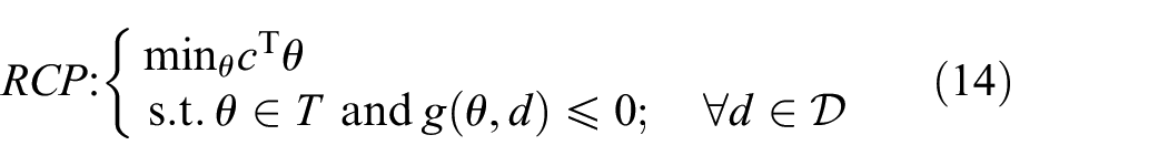
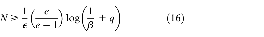
The above theorem states that if we take the number of samples appropriately, we can guarantee that the solution satisfies the robust constraint in Equation (14) on all the domain

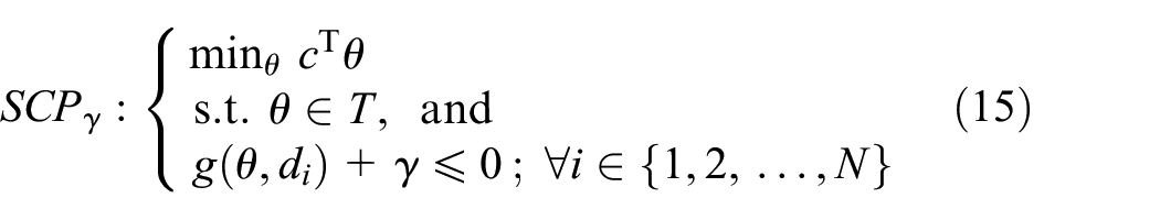
for every

computed by taking
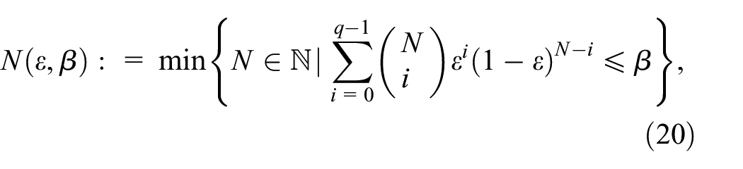
with
The above theorem is stronger than Theorem 1 in guaranteeing that the solution will be feasible for the
4. Reachability algorithms
In this section, we describe two different algorithms for computing reachable states of black-box FMI models. The two algorithms compute a scaling factor

where
The first reachability algorithm uses simulated trajectories of a black-box model and SCP to compute a maximum Lipschitz constant of the black-box model. The computed Lipschitz constant together with a central trajectory is then used for computing an interval-based approximation of the reachable set. The alternative algorithm replaces the estimation of the model’s Lipschitz constant in the previous algorithm with a solution of sensitivity equations, which describe the impact of perturbations of the system’s initial conditions on the trajectories of the system.
These algorithms are presented in detail in the following sections.
4.1. Sampling-based algorithm
For computing the reachable set from a set of initial states
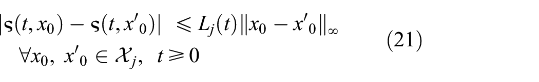
where

which gives a hyper-rectangle with center
4.1.1. RCP formulation and sampling
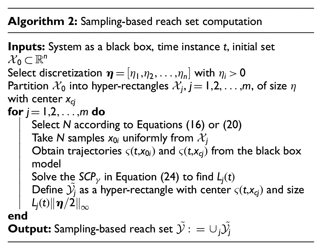
The inequality Equation (21) used in the reachability analysis can written as the RCP:
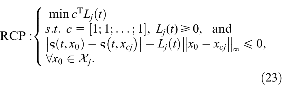
We can define the associated
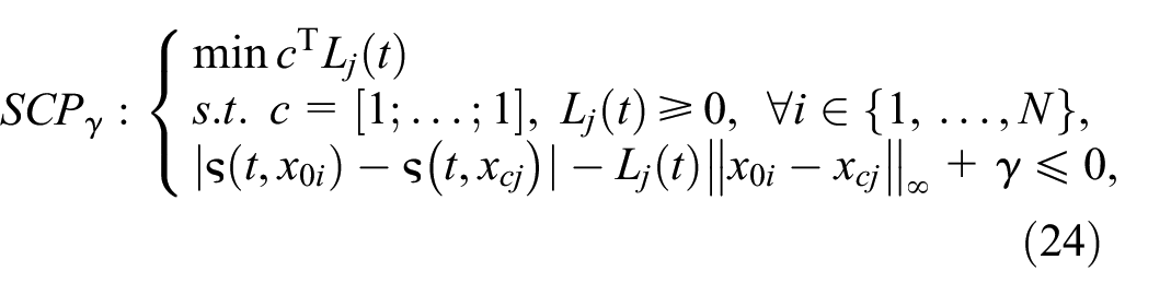
where
Once the
If
The full algorithm for our sampling-based reachability analysis is presented in Algorithm 2.
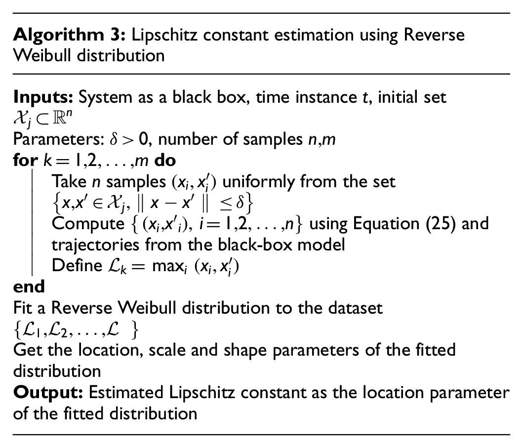
4.2. Lipschitz constant via extreme value theorem
For estimating
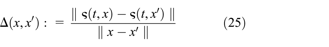
that holds for all
Let us fix a

where
Fréchet
Rvr.Weibull
where
Among the above three distributions, only the Reverse Weibull class has support bounded from above. Therefore, the limit distribution of
A procedure for estimating the Lipschitz constant is presented in Algorithm 3. This uses obtained Lipschitz constants to compute approximate reachable sets. For each state of the system, a single Lipschitz constant value is obtained from a previously sampled set. In this work, we considered two operations for obtaining a final
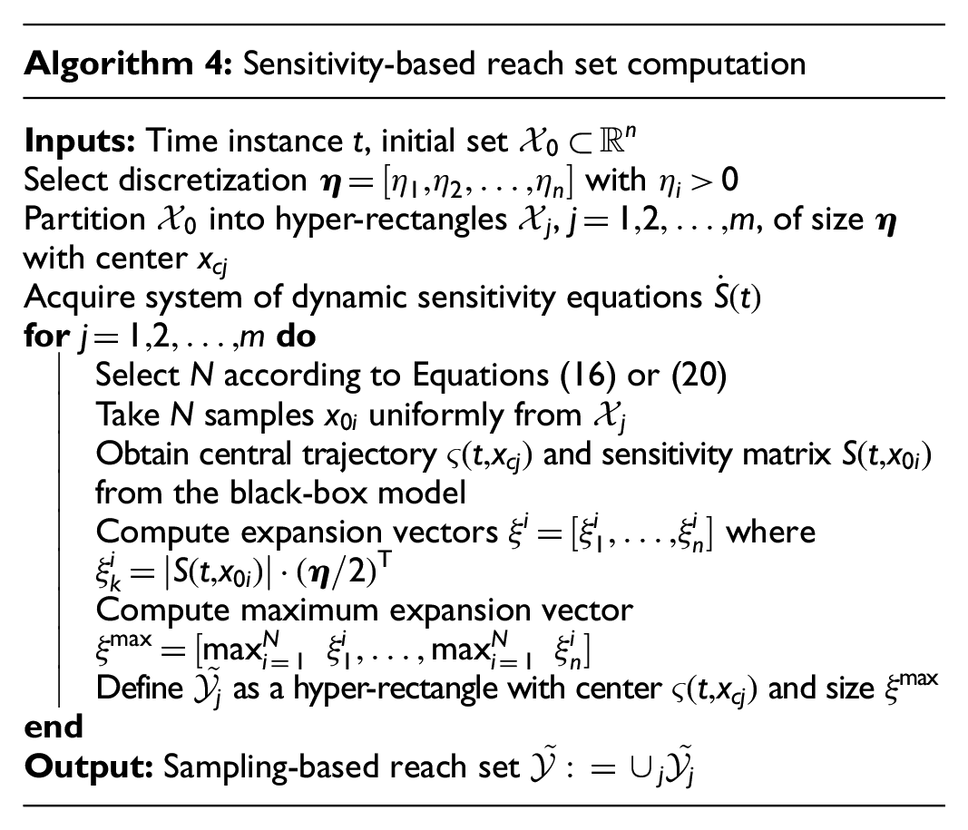
4.3. Sensitivity-based algorithm
In this section, we describe an alternative algorithm, which uses solutions of dynamic sensitivity equations to replace scaling of the initial region with a Lipschitz constant factor
The algorithm similarly partitions initial region
The reachability algorithm then over-approximates the image

which use the sensitivity matrix
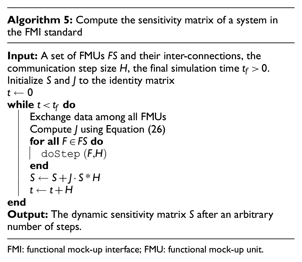
The full algorithm is described in Algorithm 4.
4.4. Building sensitivity equations co-simulation scenarios
In this section, we describe how to extend Algorithm 4 to handle networks of FMUs implementing the FMI interface.
Given the network structure of FMUs, in order to get the Jacobian matrix required to compute the sensitivity matrix, we need a way to differentiate a variable in one FMU with respect to a variable in another FMU (recall Equation (6)). For that reason, we build a dependency graph before the sampling starts. The vertex of this graph are the state variables of each FMU, their time derivatives, and the input and output variables. The edges represent the dependency of the target on the source. For example, given the system and implementation in Figure 1, its dependency graph is depicted in Figure 5.
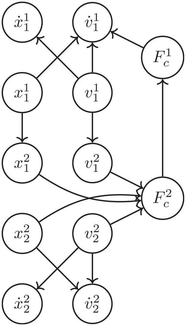
The dependency graph example of the mass spring damper example.
We can use the dependency graph to know what computations we need to do in order to calculate a derivative, as follows. Given variables
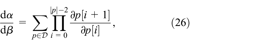
where, given path
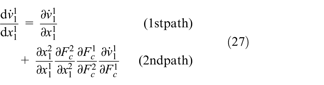
For example, in Figure 5,
In order to compute the sensitivity matrix, we initialize it to an identity matrix of the correct dimension. After that, each sample step is a co-simulation run, where we compute the Jacobian at every co-simulation step, calling a function that computes every partial derivative that makes an element of the Jacobian matrix
FMI: functional mock-up interface; FMU: functional mock-up unit.
5. Validation experiments
This section presents validation exercises that evaluate our reachability algorithms as presented in the previous section. The validation exercises cover both affine dynamical systems and nonlinear systems and aim to evaluate the conservativeness of the computed reachable sets and the associated computation time. We also obtain reachable sets (and computation time) produced by the model-based reachability tool Flow* and compare them against ones produced by our methods. To select nonlinear system benchmarks and Flow* parameters, we followed a well-known verification competition ARCH. 48
5.1. Experiment setup
All timing results in this section were measured on an HP EliteBook 840 G7 with an Intel Core i5-10310U processor under Ubuntu 22.04 (Linux 5.14.0). For the methods described in this paper, the results are based on a prototype implementation in Python. In particular, we relied on the SciPy
49
5.1.1. Affine systems
We can start to evaluate the performance of our method on Linear/Affine Initial Value Problems of form:
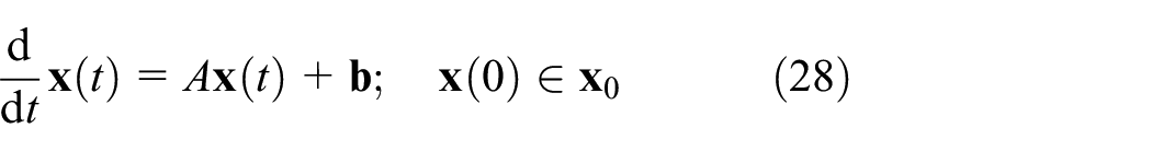
with state matrix
Sample reachability results for different classes of linear systems are shown in Figure 6. We can see that Flow* and sensitivity-based reachability analysis both produce indistinguishable flowpipes, while applying reachability analysis based on the Lipschitz constant computed from sampled trajectories alone gives a coarser reachable set estimation shown.
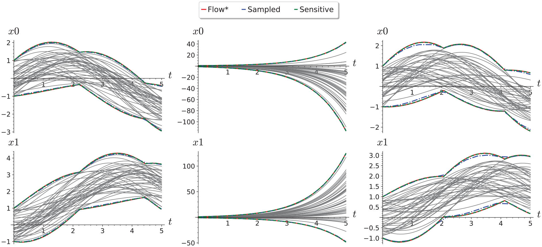
Comparison of reachability from sampled Lipschitz constants with Flow* and Sensitivity Analysis results for a randomly generated 2D stable system (left), an unstable system (middle), and an oscillator (right) from the unit initial region [−1, 1] 2 . Numerical simulations (gray) for 100 randomly sampled initial conditions are shown for comparison.
5.2. Lipschitz constant estimation accuracy
To assess the overall accuracy of our methods, we will consider uniformly randomly selected
We will assess how accurately each of the different methods captures the dynamics of the underlying system based on the vector of Lipschitz constants, which they use to compute reachable sets. While the SCP optimization directly computes a vector
Then, we may estimate the overall performance by taking the geometric mean relative absolute error (GMRAE; The geometric mean is preferred over the mean when aggregating error rates due to the latter’s sensitivity to outliers,
53
such as those arising from numerical errors when computing the RAE of small quantities.) of multiple sampled relative absolute errors

In the special case of two-dimensional (2D) systems, Figure 7 shows the evolution of the GMRAE of the Lipschitz constant vector estimate produced using dynamical sensitivity analysis, and SCP optimization for varying numbers of samples. We see that the relative error from SCP optimization decreases with an increasing number of samples, and is roughly consistent over the whole simulation time. In addition, the relative error of the method is similar between stable and unstable systems; this result is somewhat surprising given that typical Lipschitz constants for random unstable systems can be orders of magnitude larger than those of stable systems (and, indeed, the absolute error of the method will be correspondingly larger for the same number of samples). Figure 8 shows the trade-off between the total runtime of each method and the relative error achieved. We observed a relationship between the number of samples and the relative error improvement in the relative error trailing off after 80 samples. Finally, we observed that, as expected, dynamical sensitivity analysis (with a single sampled sensitivity matrix) approximates the true Lipschitz constant vector almost perfectly for linear systems, and provides by far the best accuracy/runtime trade-off for 2D systems.
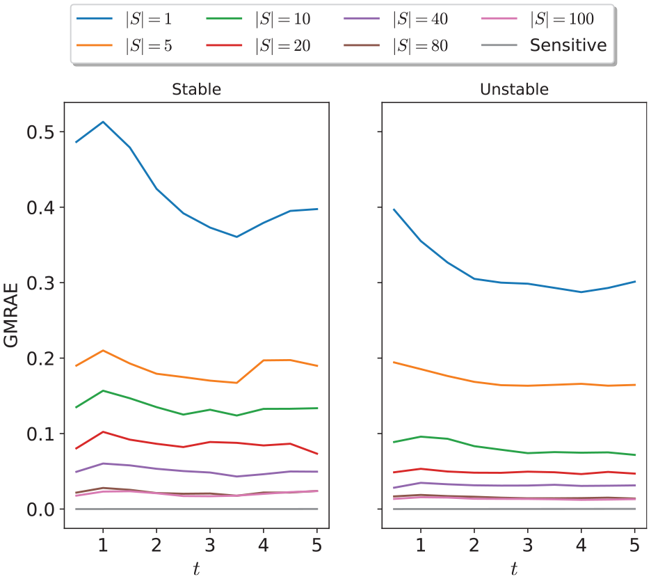
Errors of different methods of Lipschitz estimation at different time points between 1.0 and 5.0 for stable and unstable random 2D linear systems.
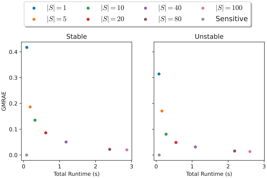
Comparison of total runtime against GMRAE for stable and unstable random 2D linear systems.
In addition, Figure 9 shows how the runtime and relative error of each method varies with the dimension of the system, based on 100 randomly sampled stable and unstable system for dimensions 1 through 6. We can see that the runtime of each method increases exponentially with the system dimension and that the rate of increase of sampling runtime increases with the number of samples, while the runtime of dynamic sensitivity analysis increases significantly more rapidly than the SCP optimization-based approximation with any of these numbers of samples. However, dynamic sensitivity consistently produced the best approximation of the system Lipschitz constant vector, and indeed, its relative error decreased with the dimension of the system. This suggests that the dynamic sensitivity equations are a reliable method of estimating the Lipschitz constant of linear systems, with consistent accuracy regardless of system dimension, while sampling offers a flexible cost/accuracy trade-off for higher-dimensional systems.
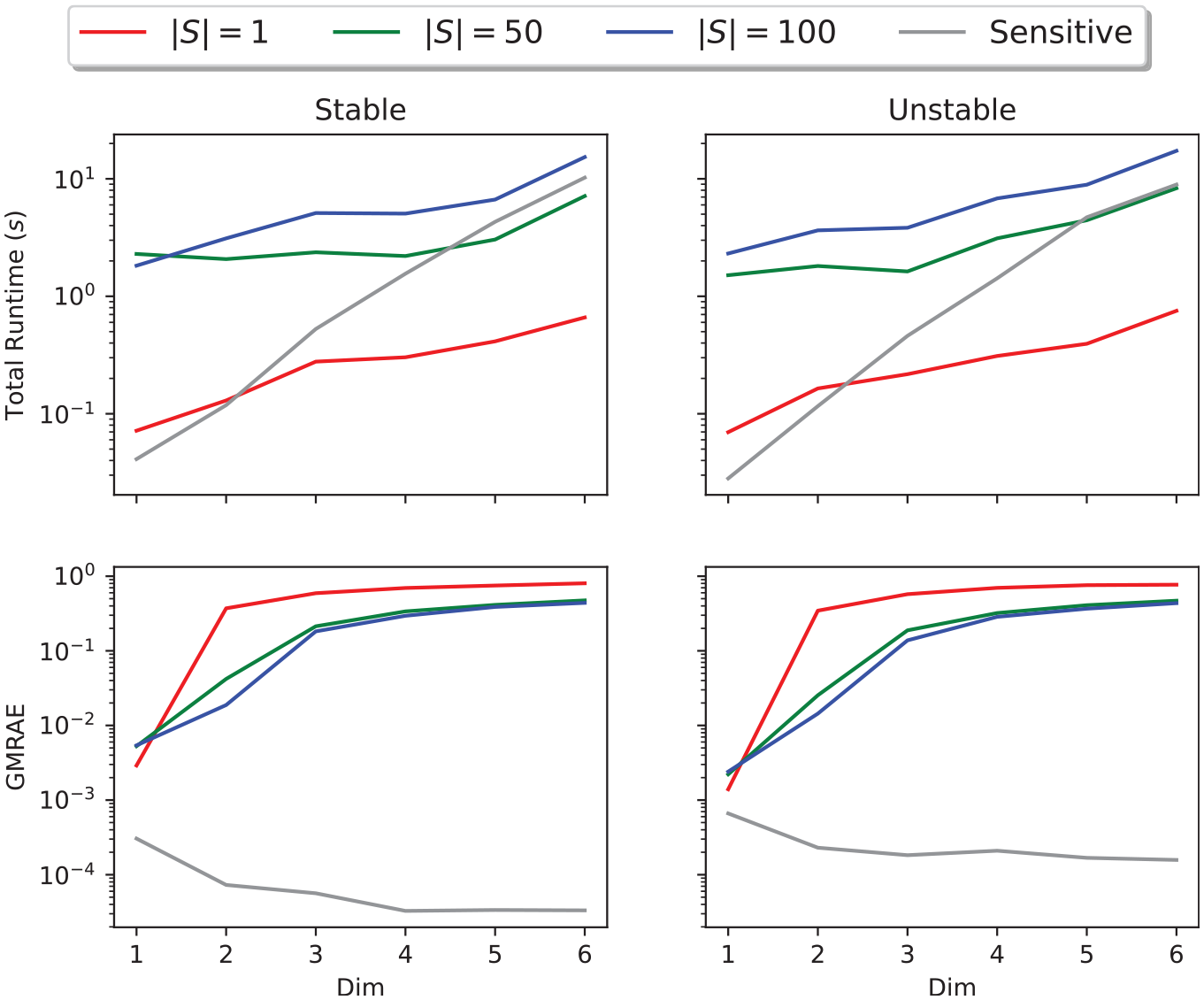
Errors and runtimes of different methods of Lipschitz estimation at time for
5.2.1. Nonlinear systems
This section compares our proposed algorithms for computing reachable sets and validates them against a model-based reachability analysis tool—Flow*. Let us start by considering 2D nonlinear Van Der Pol system as follows:
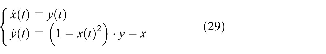
Figure 10 compares the reachable set for the initial set [1.1, 2.4] × [2.35, 3.45] computed using by Algorithms 2–4 and Flow*. The top figures show reachable sets produced by sensitivity-based Algorithm 4 (blue curve), Flow* (red curve) and some randomly sampled trajectories (gray curves) for
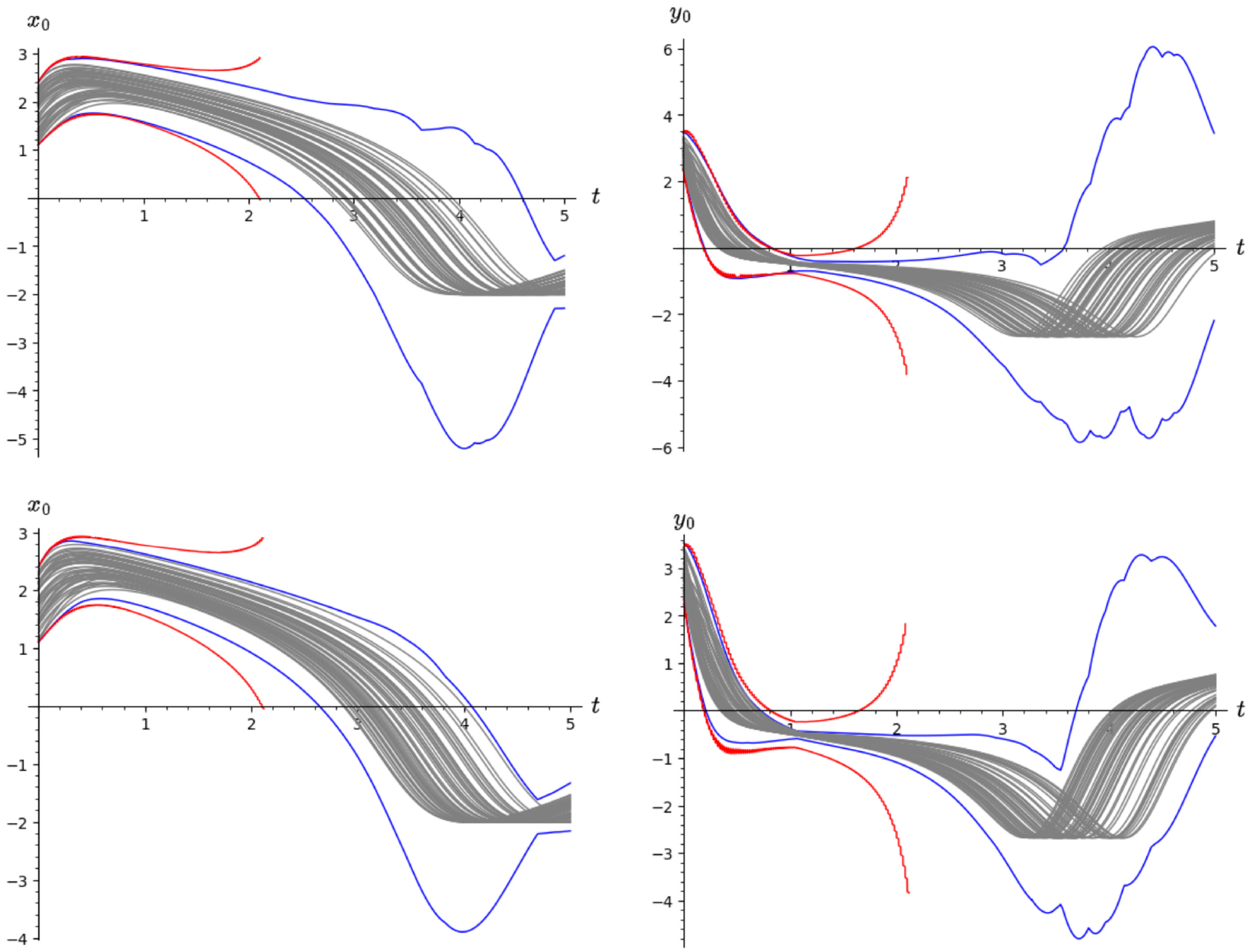
Reachable set comparison of the nonlinear Van Der Pol system for the initial set [1.1, 2.4] × [2.35, 3.45] for
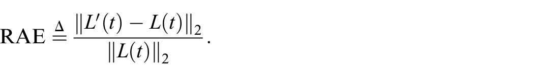
The rest of the section considers four additional nonlinear models with varying number of dimensions: coupled Van Der Pol (four-dimensional (4D)), Rossler System (three-dimensional (3D)), Spring Pendulum (4D, model from the Dynamic Sensitivity Equations section) and Biological Model (seven-dimensional (7D)). We evaluate the runtime and flowpipe volume accuracy produced by Algorithms 2 and 4. The latter is measured by using Equation (30) as follows:
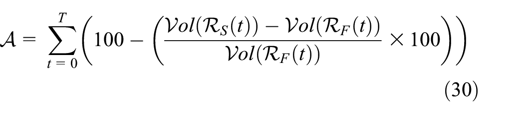
where
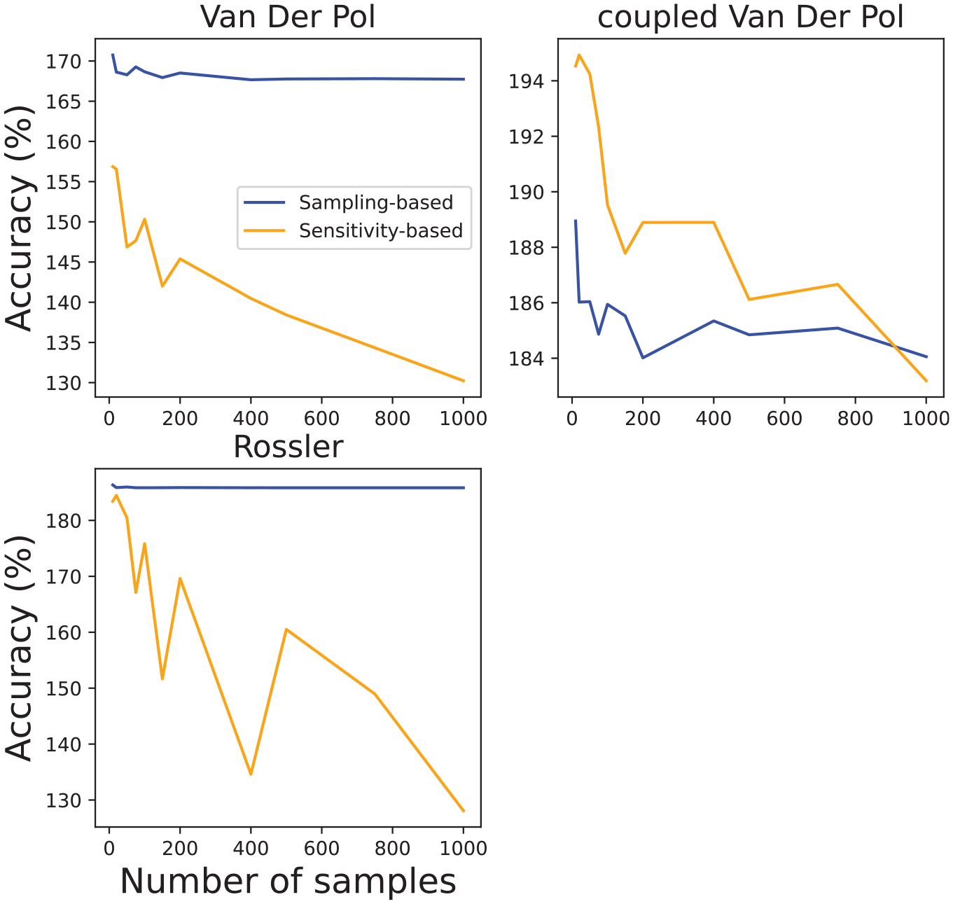
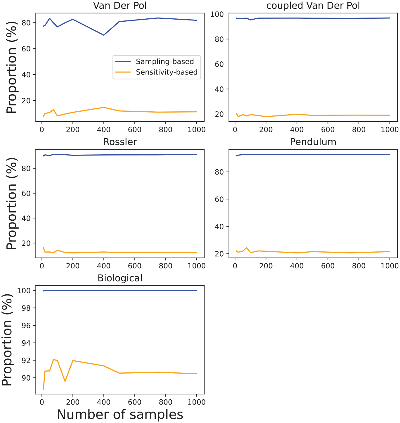
Volume error exercise that demonstrates the number of samples effects on volume accuracy. We consider the following number of samples [10, 20, 50, 75, 100, 150, 200, 400, 500, 750, 1000].
Similar findings can be observed from Figure 12 in which we summarize our accuracy results from three models for different number of samples: Van Der Pol initial state:
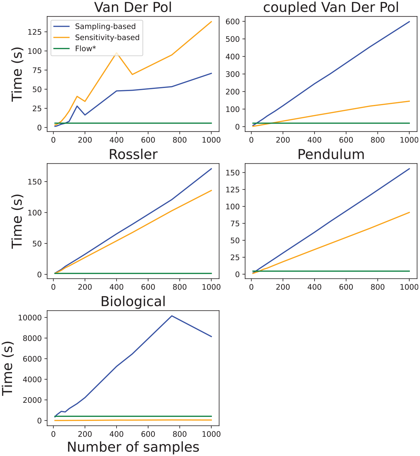
Runtime validation exercise that demonstrates the number of samples effects to computation time of reachable sets for different nonlinear models.
The runtime validation experiments are summarized in Figure 12. In these experiments, we again increased the number of samples for Algorithms 2 and 4 and observed reachable set computation time. We also include the runtime performance of the Flow* tool. Important to note that at this stage, we did not attempt to improve the computational performance of the proposed methods.
Figure 12 clearly shows that Algorithm 2 is considerably slower in comparison to Algorithm 4 and does not scale well with an increased number of samples. The main reason for this is the computation overhead of solving
The proportion of runtime in Figure 12 to perform sampling and solving SCP in Algorithm 2, and sample and solve sensitivity equations in Algorithm 4.
In short, the results presented in this section have shown that our algorithms produce reasonably conservative reachable sets for nonlinear systems. Although, with the current algorithm implementation, their runtimes do not scale well with the increased number of samples, we have shown accurate results can be produced even with a fairly small number of samples. The main limitation of the Algorithm 2 is the need for a larger number of samples to provide probabilistic accuracy guarantees, while solving SCP is a major contributor to a large runtime. The sensitivity-based algorithm provides much less conservative results but offers a more scalable approach.
5.2.2. Sensitivity matrix co-simulation
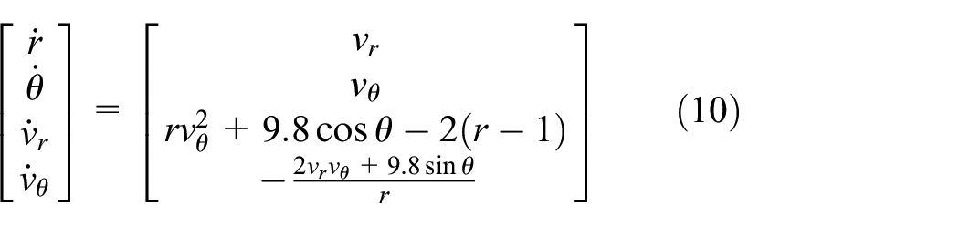
In order to validate the results of the algorithms given in “Building sensitivity equations co-simulation scenarios,” we are going to use the mass spring damper system visualized in Figure 1. The equations that describe this system’s behavior are provided in Equation (31):
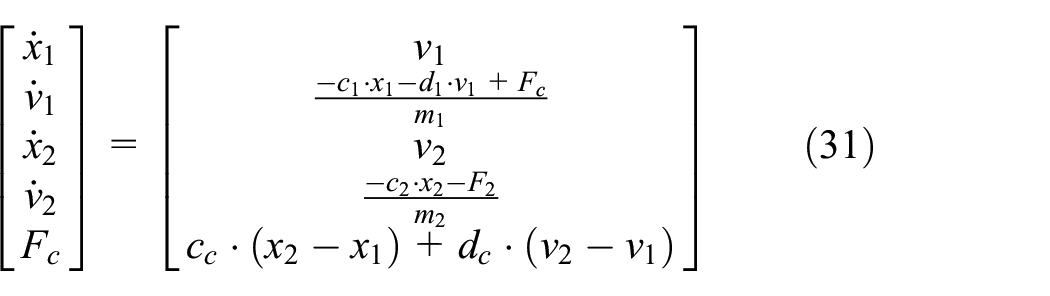
We are going to solve this system together with the coupled sensitivity equations using the SciPy solve ivp solver. In Figure 14, we validate the value of

where
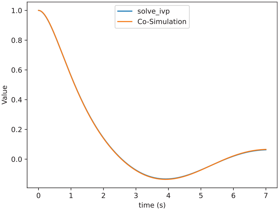
Comparison of
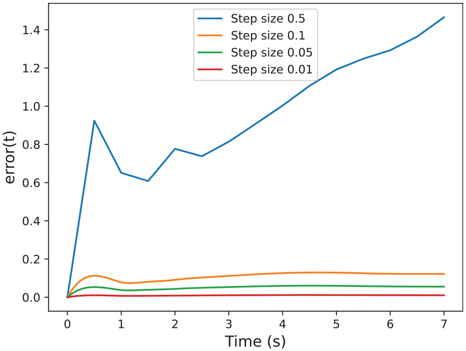
Errors between the sensitivity matrix computed by Algorithm 5 and
We can see in the results that our approximation is close enough to the solve_ivp function. Figure 14 shows that both functions are almost indistinguishable. Furthermore, Figure 15 shows that by decreasing the step size of the co-simulation scenario we can reduce the error, which allows us to get as close as we want to standard numerical algorithms.
5.2.3. Validation discussion
In this section, we explored the ability of each of our methods to accurately and efficiently approximate the dynamics of black-box models and to conservatively compute reachable sets.
First, we saw that in the case of linear systems, the sampling-based approach is able to approximate the sensitivity of the system to its initial conditions (as captured in the vector of Lipschitz constants), and the accuracy of this approximation can be increased by increasing the number of samples. This is consistent with Theorem 3, which specifies the number of samples required to achieve a given probability of over-approximating the true Lipschitz constants and, consequently, the true reachable set. We also saw that for linear systems, dynamic sensitivity analysis gives an almost exact approximation of the true Lipschitz constants regardless of system dimension, although its runtime increases rapidly with the dimension of the system.
For nonlinear systems, both sampling and dynamic sensitivity analysis give approximate results, while their conservativeness can both be increased by increasing the number of samples used. For most of our systems, we saw that dynamic sensitivity analysis gives reasonable results for a reasonably low runtime. However, the sampling-based approach is able to give more conservative results for higher numbers of samples and is also able to give probabilistic guarantees on containment.
We also saw how we can do sensitivity analysis to decoupled FMUs, by dynamically tracking the sensitivity matrix of the system. This is limited by the fact that our current co-simulation technique relies on the Forward Euler method, which produces larger errors than more competitive numerical integration methods. The use of better numerical methods is important to reduce these errors, but this would impose additional requirements on the FMUs being simulated. In practice, we observed relatively small errors between the sensitivity matrices computed via this method and the conventional open-box method using the LSODA solver.
6. Conclusion and future work
Ensuring the dependability of DTs relies on proving that the formal system models underpinning them are safe. In some cases, accurate models of complex systems are too difficult to obtain or unavailable due to IP protection (as facilitated by the FMI standard). In this work, we develop methods to provide formal analysis for models featuring uncertainty or unavailability of their dynamics, by introducing algorithms for performing reachability analysis of black-box models. We were particularly focused on the FMI standard-based black box dynamical system models. The developed data-driven and dynamic sensitivity–based reachable set computation methods have been thoroughly evaluated for linear and nonlinear dynamical systems, and results have shown that conservative reachable sets can be computed. Although, as discussed, for large numbers of samples and high-dimensional systems, the runtime performance of the algorithms offers scope for improvement (particularly the sampling-based algorithm), we saw that algorithms do not require a large number of samples to produce accurate reachable sets.
There are several interesting directions for future work:
We could investigate extending each of the methods proposed in this paper from reachability analysis, to monitoring Signal Temporal Logic properties of the system’s behavior following the methodology of Wright and Stark. 54 This would allow us to verify whether black box models satisfy high-level temporal logic specifications, while accounting for the impact of uncertainty on the result of verification via three-valued logic and probabilistic guarantees.
We could investigate the application of each of the methods to parametric black-box models, as a way to soundly account for the impact of uncertain model parameters on the behavior of the system.
Our sampling-based approach can in general be applied to hybrid models as long as trajectories are continuous functions of the initial state. To apply the dynamic sensitivity–based approach to hybrid automata, we would like to investigate how dynamic sensitivity equations could be obtained for a black-box hybrid system.
In our future work, we also aim to explore the integration of our proposed method with the DT system and replace simulations with data obtained from the physical asset. A similar approach has been presented in work by Van Acker et al. 55
Footnotes
Funding
Thomas Wright gratefully acknowledges the support of the UK EPSRC for grant EP/V026801/2, UKRI Trustworthy Autonomous Systems Node in Verifiability. The work of Sadegh Soudjani is supported by the following grants EPSRC EP/V043676/1, EIC 101070802, and ERC 101089047.