Sage Journals: Discover world-class research

Abstract

Software with increasingly complex structures plays a vital role in our lives, and our dependence on it continues to grow. As software failures and defects can cause serious problems, it is critical to measure and improve software reliability. Previous software reliability models were derived under the assumption that no failures exist at the initial point in time. However, this study developed a model that predicts software failures by setting the observation point to the initial stage and assuming that a certain number of defects already exist. Various possibilities for this have been proposed. These possibilities can arise in increasingly complex and diverse software. The proposed model assumes that software failures are not only independent it also assumed that software failures occur in a dependent manner. To demonstrate the superiority of the proposed model, we compared it with 15 traditional models across three datasets using nine criteria. The results confirmed the excellence of the proposed model by demonstrating that it achieved the best performance across all datasets. The results of this study contribute to enhancing software reliability by enabling investigation into what causes problems at the beginning of software development and creating software reliability models that are applicable in the real-world.

Keywords

Nonhomogeneous Poisson process software reliability model dependent failures initial faults

Introduction

Software plays diverse roles in all fields. It performs basic functions in many areas, from simple document processing, calculations, and repetitive tasks to specialized programs, such as statistical analysis, image and video editing, and web browsers. It also oversees all systems such as databases and operating systems. The advancement of generative AI technology has further expanded the role of software, and experts expect its importance to grow even more in the future. In today's environment, in which software has become increasingly crucial, the impact of software defects and failures can be significant. Even a minor flaw can potentially disrupt the entire system and cause widespread social disruption.

In 2017, the Equifax data breach occurred. The cause was announced to be failure to apply for a vulnerability patch. This stemmed from the problem of not patching a known vulnerability in a timely manner. Based on this, the data breach occurred along with various other causes, including inadequate network segmentation and expired certificates. Consequently, the personal information of approximately 143 million U.S. citizens was compromised. This causes extremely serious damage, as it exceeds the recorded monetary losses and carries the potential for future harm.^1,2

Although identifying and addressing the causes of software failures is crucial, predicting and preparing for software defects before they occur are equally vital. To assess this, software reliability, which measures how long software can operate without failure, was calculated. Software reliability has been calculated through software failure prediction using various research methodologies such as time-series models and failure rate models.^3,4 Among these, the software reliability model based on the nonhomogeneous Poisson process is a representative research methodology for improving software reliability. It assumes that the number of failures and defects occurring per unit time is not constant, but exhibits a time-dependent relationship. This methodology originated from research by Goel and Okumoto in 1979, which assumed that the cumulative occurrence of software failures and defects over time follows an exponential function.⁵ It has since been expanded to include studies assuming that failures and defects occur in various forms such as S-shaped, concave, and convex patterns.^6,7 Furthermore, research has been conducted to enhance software reliability through detailed failure prediction using assumptions tailored to increasingly complex software environments such as operational uncertainty and imperfect debugging.^8–10

This study extends this approach by proposing a new type of software reliability model to enhance software reliability. Conventional software reliability models assume that software failures occur independently. This assumes that failure does not affect subsequent failures. However, in integrated systems, the combination of multiple software components creates a structure in which the occurrence of a defect in one software affects or causes failures in the other software.¹¹ This study proposes a software reliability model that assumes the occurrence of dependent failures or defects. Furthermore, whereas past research assumed initial software failures and derived mathematical formulas, this study developed a model that predicts failures based on an initial observation point that does not necessarily start at zero.¹² This can be described as a general situation because the test and observation points can be measured differently depending on the observation point of the analyst or software operator. Therefore, this study proposes a general software reliability model that uses dependent failures and observation time as the initial time to enhance the reliability of today's increasingly complex software.

The remainder of this article is organized as follows. The related research for software reliability model section summarizes previous research on software reliability models. In the “a new software reliability model” section, the proposed model is introduced. The numerical examples section presents the data and goodness-of-fit analysis used to evaluate the model's performance and the resulting analysis. Finally, the last section concludes the article.

Related research for software reliability model

Software reliability is the ability of a software to function without failure over an extended period.^13,14 The function used to evaluate this is defined as the probability that the software will remain operational after a specific time t. Assuming that the lifetime is a random variable T, the reliability function $R (t)$ is calculated using the probability density function $f (t)$ . This is expressed in equation (1).

R (t) = P (T > t) = \int_{t}^{\infty} f (u) d u

(1)

The reliability function $R (t)$ is judged to indicate higher reliability as it approaches one. This concept has been extended to various studies aimed at improving software reliability. Early related research employed diverse methodologies such as error injection models, failure rate models, and time-series models to enhance software reliability. Among these, software reliability models that assume a nonhomogeneous Poisson process, in which the number of software failures occurring per unit time is not constant, have been actively researched. In 1979, Goel and Okumoto assumed that cumulative software failures increase exponentially.^5,15 Building on this, Yamada and Ohba (1983) and Ohba (1984) extended it to a software reliability model, assuming an S-shaped curve, where cumulative software failures are initially few, then increase explosively, followed by a decrease in the growth rate.^16,17

Research has also been conducted on models that reflect the various efforts invested during the testing phase to determine whether software failures will occur. Yamada et al. (1986) proposed a model that incorporated the testing effort required to correct defects discovered during the testing phase, including manpower, time, and CPU.¹⁸ Huang et al. (2007) integrated a logistic failure detection rate function with an S-shaped curve into a software reliability model.¹⁹ This curve shows that under variable testing effort conditions, the effectiveness of fault-detection diminishes as testing progresses beyond the early and middle stages. Peng et al. (2014) proposed a model in which the occurrence of simple software failures depends on both time and testing effort.²⁰ They defined this as a cumulative effort function and developed a model in which resource input patterns, such as manpower, time, and CPU, were reflected in the defect detection process. This model also considers imperfect debugging in which new defects can potentially arise.

Many studies have assumed a complete debugging model in which all faults and defects are corrected upon detection. However, it is extremely difficult to correct all the faults and defects in real environments, and it is unrealistic to prepare for every possibility. Therefore, research has been conducted on software reliability models that assume imperfect debugging to reflect realistic scenarios. These models assume that when errors are corrected, they may not be perfectly corrected or that additional errors may arise from the original error. Yamada et al. (1992) assumed that software defects and failures occur at a constant rate per unit time.²¹ They modified the form of the software failure number function to derive a software reliability model that incorporated imperfect debugging. Pham and Zhang (1997) and Pham et al. (1999) proposed a model assuming that the number of software defects and failures occurring per unit time increases according to an S-shaped curve over time.^22,23 Roy et al. (2014) proposed a model with an exponentially increasing defect function and a constant defect detection rate per unit time.²⁴ This reflects the rapid increase in defects early in testing, followed by a gradual increase as the efficiency improves over time. Pham (2007) assumed imperfect debugging and derived a model using functions in which both the defect detection rate and total number of faults gradually increase over time.¹² The test-start condition of the model assumes an arbitrary initial point. This model assumes that defects may be detected at the beginning of testing, thereby providing a more generalizable approach.

The software released a testing phase to maximize improvements before calculating the optimal release timing for deployment. However, even the released software experiences defects and failures owing to differences between the actual and test environments. These failures incur higher costs than those incurred during testing, ultimately yielding poor results. Therefore, a software reliability model that considers the uncertainty of the operating environment, including the randomness arising from the differences between the actual and test environments, was developed. Teng and Pham (2006) proposed the incorporation of an operating environment uncertainty parameter that follows a gamma distribution into the differential equation of an existing model.²⁵ Building on this work, Honda et al. (2017) and Asraful Haque and Ahmad (2021) conducted studies in which the failure detection rate function followed an S-shaped curve.^26,27 Chang et al. (2014) proposed a composite assumption software reliability model. This model simultaneously assumes testing coverage and operating environment uncertainties.²⁸ Song et al. (2017) expanded the model developed by Teng and Pham by creating a model in which the failure rate per unit time followed an S-shaped curve with three parameters.²⁹ Furthermore, it converts the uncertainty parameter of the operating environment, which follows a gamma distribution, and the fault-detection rate function into a testing coverage function.

The reliability of software is enhanced by models that assume dependent failure occurrences. This is because of the increasingly complex nature of software owing to technological advancements. This assumes that software errors affect other types of errors. Huang et al. (2006) presented a model that integrated defect dependency and debugging time delay.¹¹ This model incorporates parameters for defect dependency and removal rate, as well as parameters for delay time. Chatterjee et al. (2021) focused on dependent defects arising from imperfect debugging under defect dependency, which is a type of defect that can occur during software operation.³⁰ Their model considered the impact of change points caused by alterations in test strategies and environments during the evolution of software through testing. Samal et al. (2024) extended this research by proposing a model that considered defect dependency detection, imperfect debugging, and the maximum number of defects present in the system.³¹ Additionally, Hussain et al. (2025) conducted research assuming both complex software structures and differences between actual and test environments.³²

Among the introduced models, the model proposed by Pham (2007)¹² is novel and reflects realistic problems. This model assumes that testing in the software development phase does not always start from $t = 0$ , but rather includes a scenario where $m_{0}$ defects are already detected at the initial testing stage $t_{0}$ . Therefore, increasingly detailed assumptions were added, expanding the research into SRGMs to improve software reliability. This study proposes a model that reflects realistic conditions through such initial condition assumptions. It assumes general situations, while simultaneously proposing a model that considers the occurrence of dependent defects in software with complex structures.

A new software reliability model

This study presents a software reliability model that assumes a nonhomogeneous Poisson process to improve software reliability. Unlike a Poisson process, a nonhomogeneous Poisson process does not have a constant mean failure rate $λ$ . Instead, a mean value function, $m (t)$ is followed, which represents the mean number of failures from time $0$ to time t. A structure is implied where the number of software failures occurring per unit time is transformed into a function rather than a constant, as shown in the following equation (2).³³

Pr {N (t) = n} = \frac{{m (t)}^{n}}{n!} e^{- m (t)}, n = 0, 1, 2, \dots, t \geq 0

(2)where

N (t)

is the total number of failures up to time t, and the probability of

N (t)

being n is calculated using the Poisson process. The mean value function

m (t)

is derived through integration from the intensity function

λ (t)

, which represents the instantaneous failure rate function at time t. Reliability is assessed through this process. The mean value function

m (t)

is derived using the following differential equation (3).⁵ Here,

a (t)

denotes total expected number of failures function, and

b (t)

represents the fault detection rate function.

\frac{d m (t)}{d t} = b (t) [a (t) - m (t)]

(3)

Dependent failure software reliability model

Many previous software reliability models have assumed that software failures and faults occur independently, with one failure not affecting the other. However, software has become vastly complex, encompassing everything from the smallest components to the entire system. When a defect occurs in such complex software, the resulting failure causes dependent failures within the software. A dependent failure indicates that a failure increases the probability of other failures occurring either by directly affecting other failures or by affecting failures in other complexly integrated software components. This manifests as either a common-cause failure, where multiple software components fail simultaneously due to a single cause, or a dependent failure, where a failure in one software component within the overall system affects other software components as well.^34,35 To model this, we assume a dependent defect occurrence using differential equation (4).

\frac{d m (t)}{d t} = b (t) [a (t) - m (t)] m (t)

(4)

This assumes a dependent defect occurrence through a structure in which the mean value function $m (t)$ is multiplied once more in equation (3), identical to $a (t)$ and $b (t)$ described earlier. By multiplying m(t), the number of defects already defaulted influences the number of subsequent defaults. That is, the fault detection rate b(t) and the number of defects m(t) at the previous time point interact to influence the next time point. This study proposes the most fundamental model by setting $a (t) = a$ and $b (t) = b$ . Past software reliability models assume an initial value of $m (0) = 0$ , which expands, as shown in equation (5).

\begin{aligned} \frac{d m (t)}{d t} = b [a - m (t)] m (t) \\ \frac{1}{[a - m (t)] m (t)} d m (t) = \frac{1}{a} (\frac{1}{m (t)} + \frac{1}{a - m (t)}) d m (t) \\ = b d t \end{aligned}

(5)

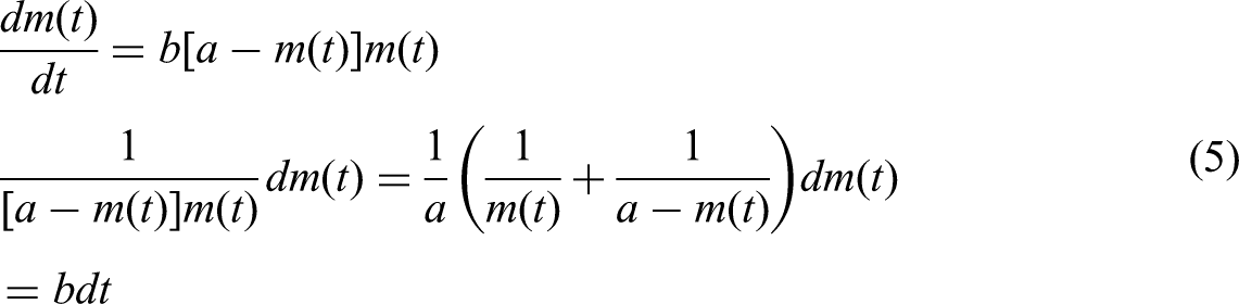
Integrating both sides of equation (5) yields equations (6–8) as follows:

\begin{aligned} \int \frac{1}{[a - m (t)] m (t)} d m (t) = \frac{1}{a} \int (\frac{1}{m (t)} + \frac{1}{a - m (t)}) d m (t) \\ = \frac{1}{a} (\ln | m (t) | - \ln | a - m (t) |) \\ = \frac{1}{a} \ln | \frac{m (t)}{a - m (t)} | \end{aligned}

(6)

\int b d t = b t + C

(7)

\ln | \frac{m (t)}{a - m (t)} | = a b t + C^{'}

(8)

Simplifying equation (8) to $m (t)$ yields the structure shown in equation (9):

\frac{m (t)}{a - m (t)} = \exp (C^{'}) \exp (a b t)

m (t) = \frac{a \exp (C^{'}) \exp (a b t)}{(1 + \exp (C^{'}) \exp (a b t))}

(9)

To define the integration constant, we assume an initial value $m (0) = 0$ , which leads to equation (10) and the past software reliability model.

\begin{aligned} m (0) = 0 \\ = \frac{a \exp (C^{'}) \exp (a b * 0)}{(1 + \exp (C^{'}) \exp (a b * 0))} \\ = \frac{a \exp (C^{'})}{(1 + \exp (C^{'}))} \\ \exp (C^{'}) = 0 \end{aligned}

(10)

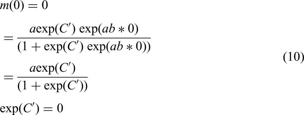
Substituting the integration constant obtained from equation (10) into equation (9) yields equation (11).

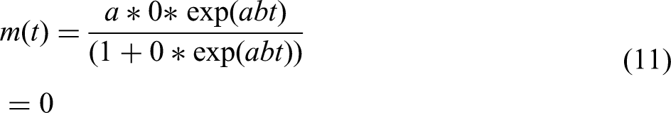
\begin{aligned} m (t) = \frac{a * 0 * \exp (a b t)}{(1 + 0 * \exp (a b t))} \\ = 0 \end{aligned}

(11)

Assuming $m (0) = 0$ , multiplying by zero continuously in equation (4) ultimately results in $m (t) = 0$ , which renders the definition invalid. Furthermore, this approach yields $m (t) = 0$ for arbitrary initial values and measured initial value, $m (t_{0}) = 0$ . Therefore, to accommodate the assumption of dependent defects, the model must be derived by assuming that the initial value or time is not 0.

Proposed dependent failure software reliability model

To address the issue of the final model $m (t) = 0$ when the initial time point is $0$ , this study assumes that the initial value $m (t_{0})$ is not zero, but $m_{0}$ .¹² Here, $t_{0}$ signifies that the starting point for testing is an arbitrary time, $t_{0}$ , which is not zero. Furthermore, it was assumed that $m_{0}$ defects (not zero) were found in the initial stage, including defects that occurred before the formal testing phase began. This assumption is more realistic than the previous assumptions because it considers defects that occur when deployed in real environments. The derivation process is shown in equation (12).

\begin{aligned} m (t_{0}) = m_{0} \\ = \frac{a \exp (C^{'}) \exp (a b t_{0})}{(1 + \exp (C^{'}) \exp (a b t_{0}))} \\ m_{0} (1 + \exp (C^{'}) \exp (a b t_{0})) = a \exp (C^{'}) \exp (a b t_{0}) \\ m_{0} = a \exp (C^{'}) \exp (a b t_{0}) - m_{0} \exp (C^{'}) \exp (a b t_{0}) \\ m_{0} = (a - m_{0}) \exp (C^{'}) \exp (a b t_{0}) \\ \exp (C^{'}) = \frac{m_{0}}{(a - m_{0}) \exp (a b t_{0})} \end{aligned}

(12)

Substituting equation (12) into equation (9) yields the final model equation proposed in this study, given by equation (13) as follows:

\begin{aligned} m (t) = \frac{a \frac{m_{0}}{(a - m_{0}) \exp (a b t_{0})} \exp (a b t)}{(1 + \frac{m_{0}}{(a - m_{0}) \exp (a b t_{0})} \exp (a b t))} \\ = \frac{a \frac{m_{0}}{(a - m_{0})} \exp (a b (t - t_{0}))}{(1 + \frac{m_{0}}{(a - m_{0})} \exp (a b (t - t_{0})))} \\ m (t) = \frac{a}{1 + (a / m_{0} - 1) e^{- a b (t - t_{0})}} \end{aligned}

(13)

Here, the proposed model includes four parameters: the total number of failures a, failure detection rate b, time point $t_{0}$ , and initial number of failures $m_{0}$ . Table 1 lists the traditional nonhomogeneous Poisson process (NHPP) software reliability model proposed based on the various assumptions described in the related research for software reliability model section and the proposed NHPP software reliability model. Among the many software reliability models proposed in the past, we aimed to comprehensively compare the models proposed based on various assumptions. Models 1–4 assume that the software failures occur independently. Models 5 and 6 consider the testing effort; models 7 through 12 consider incomplete debugging; models 13 through 15 consider operational environment uncertainty; and Model 16, the new type of NHPP software reliability model proposed in this study, considers dependent failures.

Table 1.

Software reliability models.

No.	Model	Mean value function
1	GO⁵	$m (t) = a (1 - e^{- b t})$
2	HDGO¹⁵	$m (t) = l o g (\frac{e^{a} - c}{e^{a e^{- b t}} - c})$
3	DS¹⁶	$m (t) = a (1 - (1 + b t) e^{- b t})$
4	IS¹⁷	$m (t) = \frac{a (1 - e^{- b t})}{1 + β e^{- b t}}$
5	YE¹⁸	$m (t) = a (1 - e^{- γ α (1 - e^{- β t})})$
6	YR¹⁸	$m (t) = a (1 - e^{- γ α (1 - e^{- β t^{2} / 2})})$
7	YID 1²¹	$m (t) = \frac{a b}{α + b} (e^{α t} - e^{- b t})$
8	YID 2²¹	$m (t) = a (1 - e^{- b t}) (1 - \frac{α}{b}) + α a t$
9	PZ²²	$m (t) = \frac{((c + a) [1 - e^{- b t}] - [\frac{a b}{b - α}] (e^{- a t} - e^{- b t}))}{1 + β e^{- b t}}$
10	PNZ²³	$m (t) = \frac{a (1 - e^{- b t}) (1 - \frac{α}{b}) + α a t}{1 + β e^{- b t}}$
11	RMD²⁴	$m (t) = a α [1 - e^{- b t}] - [\frac{a b}{b - β} (e^{- β t} - e^{- b t})]$
12	DP2¹²	$m (t) = m_{0} (\frac{γ t + 1}{γ t_{0} + 1}) e^{- γ (t - t_{0})} + α (γ t + 1) (γ t - 1 + (1 - γ t_{0}) e^{- γ (t - t_{0})})$
13	TP²⁵	$m (t) = \frac{a}{p - q} [1 - {(\frac{β}{β + (p - q) \ln (\frac{c + e^{b t}}{c + 1})})}^{α}]$
14	TC²⁸	$m (t) = N [1 - {(\frac{β}{β + {(a t)}^{b}})}^{α}]$
15	3P²⁹	$m (t) = N [1 - (\frac{β}{β - \frac{a}{b} \ln (\frac{(1 + c) e^{- b t}}{1 + c e^{- b t}})})]$
16	New model	$m (t) = \frac{a}{1 + (a / m_{0} - 1) e^{- a b (t - t_{0})}}$

Numerical examples

Data introduction

Three datasets were used in this study. The first and second datasets are telecommunications system data, which are system test data for telecommunications systems.³⁶ Data collection was divided into two phases: Phase 1 and Phase 2. Both automated and human-involved tests were performed on multiple test beds. Phase 1 recorded 26 failures over 21 weeks, whereas Phase 2 recorded 43 failures over 21 weeks. The third dataset is a fault dataset recorded from an online communication system project at the ABC Software Company.³⁷ The project team consisted of one unit manager, one user interface software engineer, and 10 software engineers and testers. The dataset generated from this project was collected over a total of 12 weeks, during which 110 failures occurred. Error detection involves the development and testing teams prioritizing the most critical change requests and organizing them into subcategories to facilitate resolution. This allowed for classification based on severity, resulting in a dataset that simultaneously considered both major and minor issues. Table 2 presents the weekly number of observed failures for the three datasets introduced above.

Table 2.

Datasets.

Dataset1			Dataset2			Dataset3
Index	Failure	Index	Failure	Index	Failure	Index	Failure	Index	Failure
1	1	13	19	1	3	13	30	1	17
2	1	14	19	2	4	14	32	2	24
3	2	15	22	3	4	15	36	3	28
4	3	16	22	4	7	16	37	4	38
5	5	17	23	5	9	17	39	5	48
6	5	18	24	6	9	18	39	6	71
7	5	19	24	7	10	19	39	7	81
8	8	20	24	8	13	20	42	8	89
9	9	21	26	9	17	21	43	9	91
10	11			10	19			10	104
11	13			11	23			11	105
12	15			12	25			12	110

Criteria

Nine criteria were used to evaluate model performance. These criteria were calculated based on the difference between the actual data and estimated values obtained from the model. Among the nine criteria, $\hat{m} (t_{i})$ represents the estimated value, $y_{i}$ represents the actual value, n represents the number of observations, and m represents the number of parameters included in each model.

Table 3 lists the formulae for the criteria used to compare the models. The first criterion, the mean squared error (MSE), was obtained by dividing the sum of squares of the differences between the actual data and estimated values by the number of observations. The second criterion, mean absolute error (MAE), was obtained by dividing the sum of the absolute values by the number of parameters.^38,39 The third and fourth criteria, predictive ratio risk (PRR) and predictive power (PP), were defined as the difference between the actual and estimated values divided by the estimated and actual values, respectively.⁴⁰ This expresses the difference between the actual and estimated values as a ratio, and serves as a criterion to demonstrate superiority through PP. The fifth criterion is the predicted relative variation (PRV), which is the standard deviation of prediction bias. The sixth criterion, the tail statistic (TS), is the mean percentage deviation across all time points.^41,42 The seventh criterion is Akaike's information criterion (AIC), and the eighth is the Bayes information criterion (BIC).⁴³ These two metrics are used to compare the maximization of the likelihood function and are judged by the Kullback–Leibler divergence between the model and probability distribution of the data. BIC incorporates a modified form of the AIC penalty. Here, logL denotes $l o g L = \sum_{i = 1}^{n} {(y_{i} - y_{i - 1}) \ln (m (t_{i}) - m (t_{i - 1})) - (m (t_{i}) - m (t_{i - 1})) - \ln ((y_{i} - y_{i - 1})!)}$ .

Table 3.

Criteria for comparison of model.

No.	Criteria	Formula
1	MSE	$M S E = \frac{\sum_{i = 1}^{n} {(\hat{m} (t_{i}) - y_{i})}^{2}}{n - m}$
2	MAE	$M A E = \frac{\sum_{i = 1}^{n} \| \hat{m} (t_{i}) - y_{i} \|}{n - m}$
3	PRR	$P R R = \sum_{i = 1}^{n} {(\frac{\hat{m} (t_{i}) - y_{i}}{\hat{m} (t_{i})})}^{2},$
4	PP	$P P = \sum_{i = 1}^{n} {(\frac{\hat{m} (t_{i}) - y_{i}}{y_{i}})}^{2}$
5	Adj_R²	$a d j_R^{2} = 1 - \frac{(1 - R^{2}) (n - 1)}{n - m - 1}$
6	PRV	$P R V = \sqrt{\frac{\sum_{i = 1}^{n} {(y_{i} - \hat{m} (t_{i}) - \sum_{i = 1}^{n} [\frac{\hat{m} (t_{i}) - y_{i}}{n}])}^{2}}{n - 1}}$
7	TS	$TC = 100 * \sqrt{\frac{\sum_{i = 1}^{n} {(y_{i} - \hat{m} (t_{i}))}^{2}}{\sum_{i = 1}^{n} y_{i}^{2}}}$
8	AIC	$A I C = - 2 \log L + 2 m$
9	BIC	$B I C = - 2 \log L + m \log n$

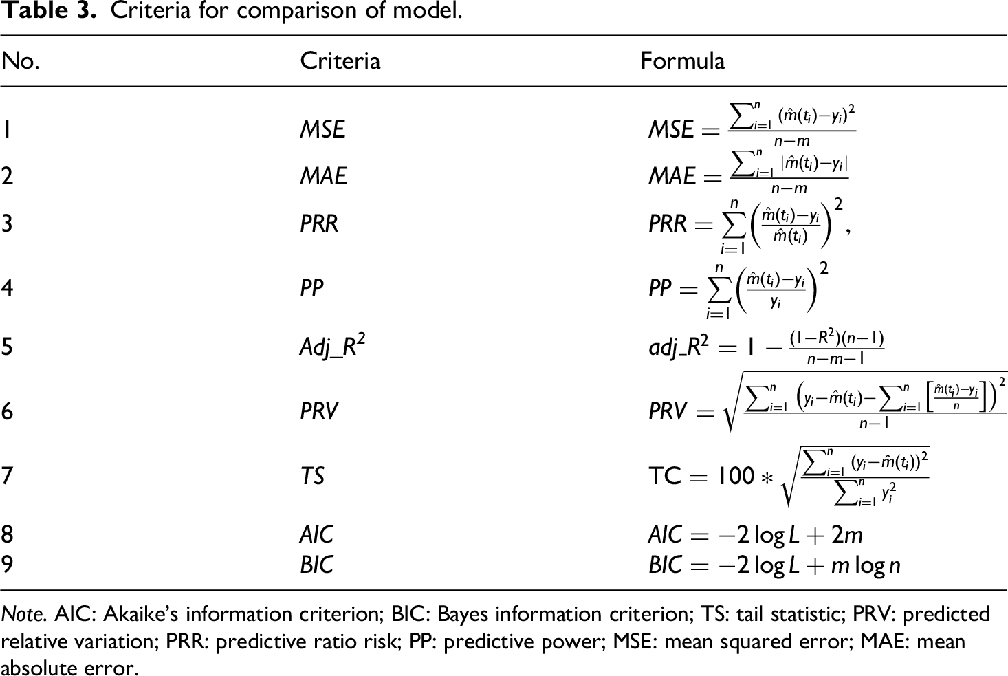
Note. AIC: Akaike's information criterion; BIC: Bayes information criterion; TS: tail statistic; PRV: predicted relative variation; PRR: predictive ratio risk; PP: predictive power; MSE: mean squared error; MAE: mean absolute error.

The ninth criterion, adj_R² is the adjusted coefficient of determination, which reflects the number of parameters in the coefficient of determination of the regression equation, $R^{2} = 1 - (\sum_{i = 1}^{n} {(\hat{m} (t_{i}) - y_{i})}^{2} / \sum_{i = 1}^{n} {(y_{i} - \bar{y_{i}})}^{2})$ .⁴⁴

Nine criteria indicated a better fit when adj_R² approached one, whereas the other eight criteria indicated a better fit when they approached zero. These nine criteria were combined to demonstrate model superiority. We estimated each model's parameters using the least squares estimation (LSE) method, which calculates the difference between the values estimated using R and Matlab and the actual data. Subsequently, we computed their fit to compare their superiority.⁴⁵

Analysis results

Analysis results for Dataset 1

Table 4 lists the parameter values estimated from Dataset 1 for the traditional NHPP software reliability models and the proposed NHPP software reliability model. The proposed model includes four parameters: the total number of failures a, failure detection rate b, time point $t_{0}$ , and initial number of failures $m_{0}$ . The estimated values are $\hat{a} = 26.2204, \hat{b} = 0.0123, {\hat{t}}_{0} = 0.0956,$ and ${\hat{m}}_{0} = 0.8106$ . The estimated total number of failures and initial number of failures accurately reflect the characteristics of Dataset 1.

Table 4.

Parameter estimation of model from Dataset 1.

Model	$\hat{a}$	$\hat{b}$	$\hat{c}$	$\hat{N}$	$\hat{α}$	$\hat{β}$	$\hat{γ}$	$\hat{p}$	$\hat{q}$	${\hat{t}}_{0}$	${\hat{m}}_{0}$
GO	2098.17	0.0006
HDGO	709.78	0.0018	0.0010
DS	39.822	0.1104
IS	26.693	0.19				21.709
YE	1270.69				6.6343	0.0005	0.3037
YR	33.920				5.5309	0.0033	0.5204
YID1	102.04	0.0106			0.0279
YID2	0.0137	0.4613			108.62
PZ	2.2722	0.3384	23.705		0.3192	39.220
PNZ	26.688	0.19			0.0000	21.707
RMD	39.593	0.1273			0.9195	0.1273
DP2					5946.46		0.0044			0.5037	3.9498
TP	0.0001	0.2850	16.461		2.7234	0.0000		0.1925	0.1925
TC	0.0677	2.2340		26.833	85396.1	61080.8
3P	1.9166	0.19	1804.74	26.857		0.0831
NEW	26.220	0.0123								0.0956	0.8106

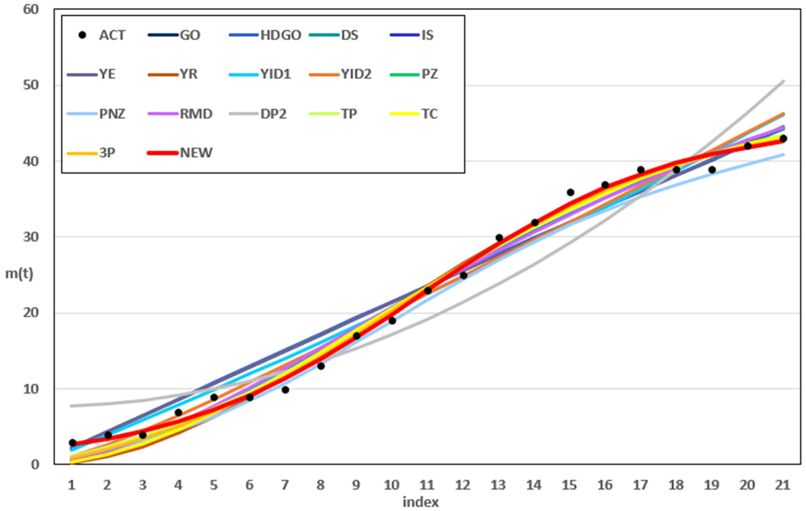
Figure 1 shows the results for the estimated values of all compared models and the cumulative number of failures in Dataset 1. The dashed line represents the actual data, whereas the thick red solid line represents the values estimated from the proposed software reliability model, which considers the initial conditions and dependent failure occurrence assumptions. The proposed model closely followed the trend of the actual data compared with the other models, showing very small differences from the actual values, except at points where failures occurred particularly frequently. Figure 2 shows the difference between actual and predicted values for Dataset 1 based on the top five models: DS, IS, PZ, PNZ, and the proposed model. Compared to other models, the proposed model yielded results closer to 0.

Figure 1.

Results for the estimated values of all compared models in Dataset 1.

Figure 2.

Difference between actual and predicted values for Dataset 1.

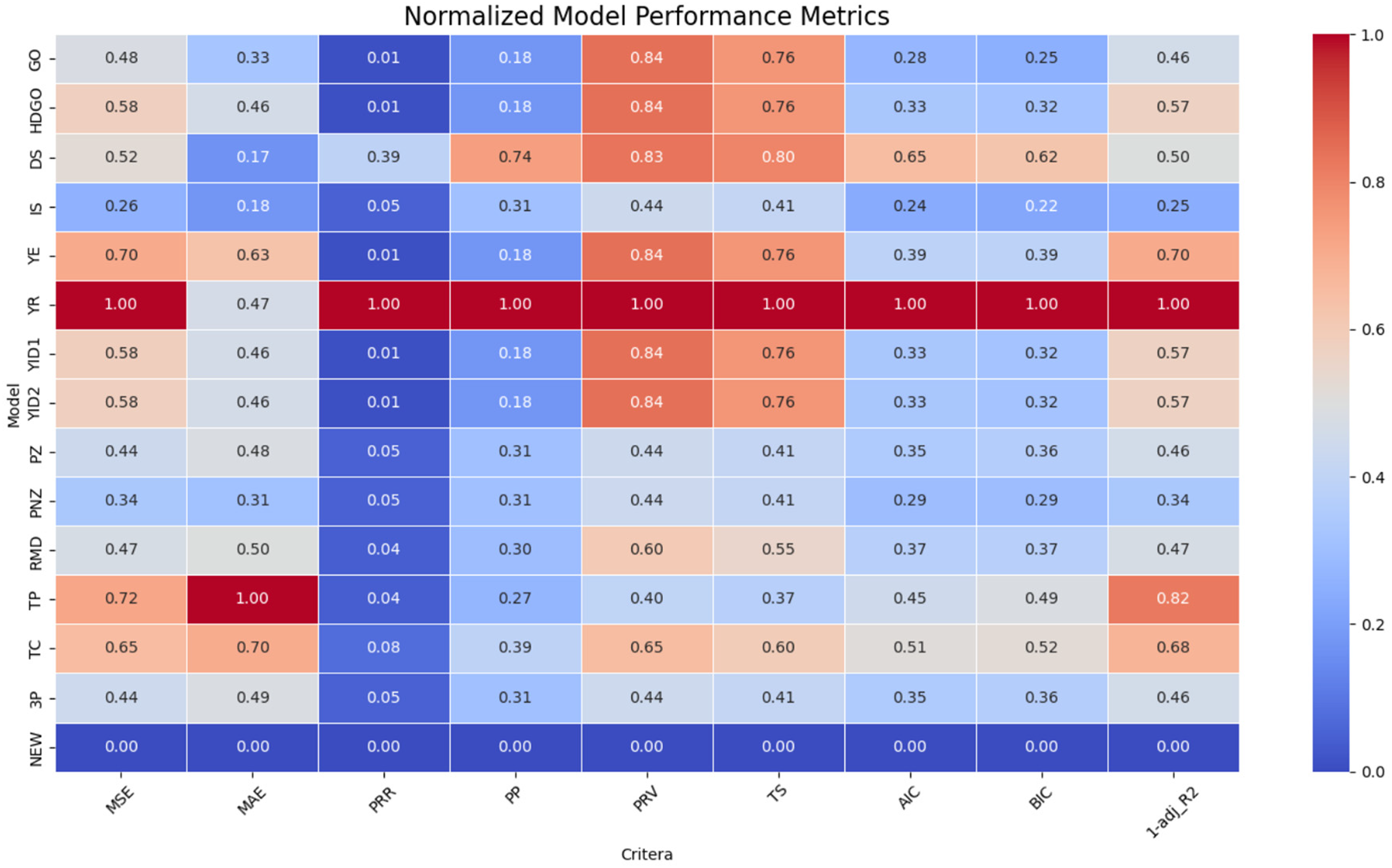
Based on the parameter estimates in Table 4, $\hat{m} (t_{i})$ is computed at each time point for all 16 software reliability models. The differences between the $\hat{m} (t_{i})$ and the actual observations $y_{i}$ for Dataset 1 in Table 2 are then substituted into the criteria presented in Table 3, and the result present in Tables 5 and 6. These results are used to evaluate and demonstrate the superiority of the 16 models. The proposed model yielded the best results for the MSE, MAE, PRR, PP, and adj_R² at 0.5883, 0.6839, 0.3551, 0.3839, and 0.9922, respectively. The PRV and TS showed the second-best results at 0.7068 and 4.3144, respectively. The AIC and BIC showed the fourth-best results at 65.7117 and 69.8898, respectively. These results demonstrated the superior performance of the proposed model. The PRV and TS yielded the best results in the PZ, and the AIC and BIC performed best in the DS. In addition, to compare the numerical values of the models and indicators, we visualized the entire set of indicators using a heatmap. The color of each cell represents the state level of the performance, and Figure 3 shows the performance indicators of each model normalized to a scale of 0 to 1. For accurate interpretation, we excluded the DP2 model, which showed significant differences in the criteria values. Because the value of adj_R² is closer to 1, the performance is better. Therefore, we converted it to adj_R² to align it with indicators such as errors, where smaller values are better. As shown in Figure 3, the new model exhibited superior overall performance.

Figure 3.

Comparison of models based on normalized metrics for Dataset1.

Table 5.

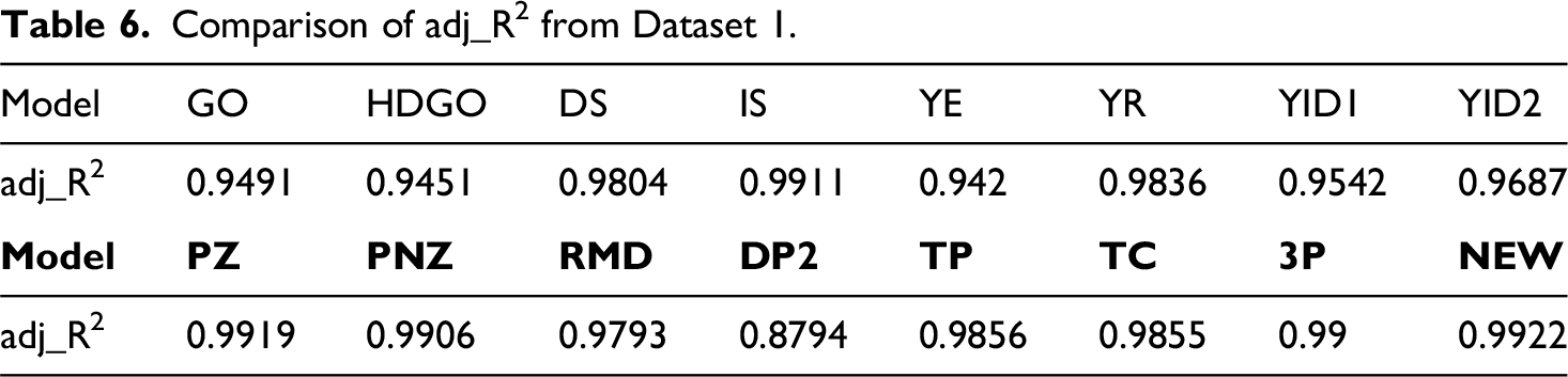
Comparison of criteria from Dataset 1.

Model	MSE	MAE	PRR	PP	PRV	TS	AIC	BIC
GO	3.8867	1.7901	1.3404	4.8978	1.8451	11.7235	65.3643	67.4534
HDGO	4.1782	1.9088	1.3687	5.0732	1.8546	11.8310	67.3774	70.5109
DS	1.4938	1.0525	12.0685	0.9676	1.1908	7.2681	63.9399	66.00
IS	0.6744	0.7192	2.8506	0.6561	0.7727	4.7533	64.1779	67.3115
YE	4.4036	2.0155	1.3592	5.0121	1.8556	11.8038	69.3732	73.5513
YR	1.2469	1.0443	28.1038	1.2144	1.0283	6.2811	67.6550	71.8331
YID1	3.4905	1.7320	0.9576	2.8125	1.7474	10.8136	67.7421	70.8757
YID2	2.3845	1.3039	5.6784	0.8561	1.4649	8.9376	67.1642	70.77
PZ	0.6096	0.7289	0.4017	0.4898	0.6972	4.2606	68.1637	73.3863
PNZ	0.7141	0.7615	2.8512	0.6562	0.7727	4.7534	66.1773	70.3554
RMD	1.5697	1.2125	162.4871	2.0626	1.1527	7.0474	69.1660	73.3441
DP2	9.1543	2.8493	2.1011	21.3552	2.7893	17.0188	78.5479	82.7260
TP	1.0762	0.9680	1.6819	0.5201	0.8678	5.53	71.7819	79.0936
TC	1.0938	1.0033	102.1779	1.7469	0.9197	5.7071	70.5608	75.7834
3P	0.7589	0.8092	2.8509	0.6561	0.7728	4.7538	68.1713	73.3939
NEW	0.5883	0.6839	0.3551	0.3839	0.7068	4.3144	65.7117	69.8898

Table 6.

Comparison of adj_R² from Dataset 1.

Model	GO	HDGO	DS	IS	YE	YR	YID1	YID2
adj_R²	0.9491	0.9451	0.9804	0.9911	0.942	0.9836	0.9542	0.9687
Model	PZ	PNZ	RMD	DP2	TP	TC	3P	NEW
adj_R²	0.9919	0.9906	0.9793	0.8794	0.9856	0.9855	0.99	0.9922

Analysis results for Dataset 2

Table 7 lists the parameter values estimated from Dataset 2 for 15 traditional models and the proposed model. The four parameters of the proposed model were $\hat{a} = 45.0207, \hat{b} = 0.00626, {\hat{t}}_{0} = 0.1769,$ and ${\hat{m}}_{0} = 2.1156$ . The estimated total number of failures $\hat{a}$ and initial number of failures ${\hat{m}}_{0}$ showed results similar to the total number of failures and initial number of failures of Dataset 2.

Table 7.

Parameter estimation of model from Dataset 2.

Model	$\hat{a}$	$\hat{b}$	$\hat{c}$	$\hat{N}$	$\hat{α}$	$\hat{β}$	$\hat{γ}$	$\hat{p}$	$\hat{q}$	${\hat{t}}_{0}$	${\hat{m}}_{0}$
GO	884.85	0.0024
HDGO	709.78	0.0031	0.7660
DS	62.304	0.1185
IS	46.544	0.2409				12.224
YE	4433.87				210.76	0.0006	0.0039
YR	46.607				25.030	0.00001	32.2
YID1	142.86	0.0135			0.0237
YID2	1.9831	0.4151			1.2008
PZ	0.0466	0.2409	46.497		32.902	12.224
PNZ	.851	0.2651			0.0247	10.220
RMD	62.484	0.1111			1.0379	0.1111
DP2					9668.76		0.0044			0.0011	7.6657
TP	39.543	0.22	11.820		4.8702	3.5013		2.0536	1.2672
TC	0.0705	1.8640		48.963	7510.55	7164.88
3P	1.1273	0.2409	9443.01	46.576		0.0066
NEW	45.021	0.0063								0.1769	2.1156

Figure 4 shows the estimated values of all the models compared and the cumulative number of failures for Dataset 2. The legend is the same as that shown in Figure 1. The results are very similar to the actual data trend compared with the other models, and the difference from the actual values at all points, except where the cumulative number of failure changes is small. Figure 5 shows the differences between actual and predicted values for Dataset 2 based on the top five models: IS, PZ, TP, 3P, and the proposed model. Compared to the other models, the proposed model yielded results closer to 0. In particular, the proposed model showed highly suitable results from the outset compared to the other four models.

Figure 4.

Results for the estimated values of all compared models in Dataset 2.

Figure 5.

Difference between actual and predicted values for Dataset 2.

Tables 8 and 9 list the results of evaluating the 16 models using nine criteria to assess the superiority of the model. The MSE, MAE, PRR, PP, PRV, TS, AIC, and BIC values were 1.1042, 0.9485, 0.1958, 0.1535, 0.9668, 3.5269, 75.603, and 79.781, respectively, which were close to zero. The value of adj_R² was 0.9943, which was the closest to 1. The proposed model demonstrated the most optimal outcomes compared with the other 15 models. Figure 6 compares the normalized metric-based models on Dataset 2 and shows that the new model performed better overall.

Figure 6.

Comparison of models based on normalized metrics for Dataset 2.

Table 8.

Comparison of criteria from Dataset 2.

Model	MSE	MAE	PRR	PP	PRV	TS	AIC	BIC
GO	6.8776	2.3227	0.6989	1.1767	2.4909	9.3058	78.09	80.3799
HDGO	7.3395	2.4646	0.70	1.2009	2.5003	9.3568	80.2845	83.4181
DS	3.2731	1.7136	44.2887	1.44	1.7479	6.4196	81.0864	83.1754
IS	1.8704	1.2203	5.9521	0.8964	1.2731	4.7234	76.9480	80.0816
YE	7.5083	2.5730	0.6920	1.13	2.4636	9.1971	82.3141	86.4921
YR	3.1991	1.6303	110.4849	1.8410	1.5954	6.0034	85.7711	89.9492
YID1	6.3419	2.	0.6772	0.7596	2.3747	8.6976	81.0712	84.2047
YID2	4.9693	2.0237	3.3818	0.7618	2.1136	7.6991	81.3400	84.4736
PZ	2.1042	1.3728	5.9519	0.8964	1.2731	4.7234	80.9480	86.1706
PNZ	6.1021	2.3255	9.8077	1.1859	1.3707	8.13	79.5564	83.7345
RMD	3.6133	1.8912	17.2252	1.1813	1.7450	6.3802	83.2248	87.40
DP2	20.6436	4.4201	1.3778	5.2640	4.1886	15.2501	96.1337	100.3118
TP	2.5657	1.6987	4.2181	0.7684	1.3314	4.8789	84.8094	92.1211
TC	3.3003	1.8034	57.2558	1.5783	1.5894	5.9155	86.4436	91.6662
3P	2.1042	1.3728	5.9521	0.8964	1.2731	4.7235	80.9480	86.1706
NEW	1.1042	0.9485	0.1958	0.1535	0.9668	3.5269	75.6025	79.7806

Table 9.

Comparison of adj_R² from Dataset 2.

Model	GO	HDGO	DS	IS	YE	YR	YID1	YID2
adj_R²	0.9647	0.9623	0.9832	0.9904	0.9613	0.9835	0.9674	0.9744
Model	PZ	PNZ	RMD	DP2	TP	TC	3P	NEW
adj_R²	0.9891	0.9685	0.9814	0.8935	0.9866	0.98	0.9891	0.9943

Analysis results for Dataset 3

Table 10 lists the parameter values estimated from Dataset 3 for the 16 models. The parameters for the proposed model are as follows: $\hat{a} = 114.5245, \hat{b} = 0.003919, {\hat{t}}_{0} = 0.4629,$ and ${\hat{m}}_{0} = 11.6309$ . Similar to the other datasets, the results were comparable to the initial and total numbers of failures.

Table 10.

Parameter estimation of model from Dataset 3.

Model	$\hat{a}$	$\hat{b}$	$\hat{c}$	$\hat{N}$	$\hat{α}$	$\hat{β}$	$\hat{γ}$	$\hat{p}$	$\hat{q}$	${\hat{t}}_{0}$	${\hat{m}}_{0}$
GO	274.626	0.04511
HDGO	274.626	0.04511	0.01544
DS	126.246	0.911
IS	121.818	0.32477				3.9944
YE	12104.5				5.4785	0.0443	0.0042
YR	140.5				4.4820	0.0274	0.3830
YID1	264.863	0.04680			0.0014
YID2	274.611	0.04511			0.0000
PZ	0.00136	0.32477	121.818		0.0546	3.9943
PNZ	121.060	0.32541			0.0005	3.9812
RMD	109.008	0.21792			1.3184	0.2179
DP2					70173.7		0.0043			1.8746	33.584
TP	0.00838	0.22783	13.9369		1.419	0.0019		1.0995	1.0994
TC	0.11119	1.35785		136.141	12527.9	10763.5
3P	1.23184	0.32491	184.943	123.408		0.1032
NEW	114.524	0.00392								0.46	11.631

Figure 7 shows the estimated values of all compared models and the cumulative number of failures for Dataset 3. It has the same legend as that shown in Figure 1. Similar to the other datasets, the results closely resembled the actual data trend, showing a very small difference from the actual values. Figure 8 shows the difference between actual values and predicted values for Dataset 3 based on the top five models (IS, PZ, PNZ, 3P, and the proposed model). Unlike other models, the proposed model exhibited a trend close to 0 from the outset because it reflected results assuming an initial number of failures.

Figure 7.

Results for the estimated values of all compared models in Dataset 3.

Figure 8.

Difference between actual and predicted values for Dataset 3.

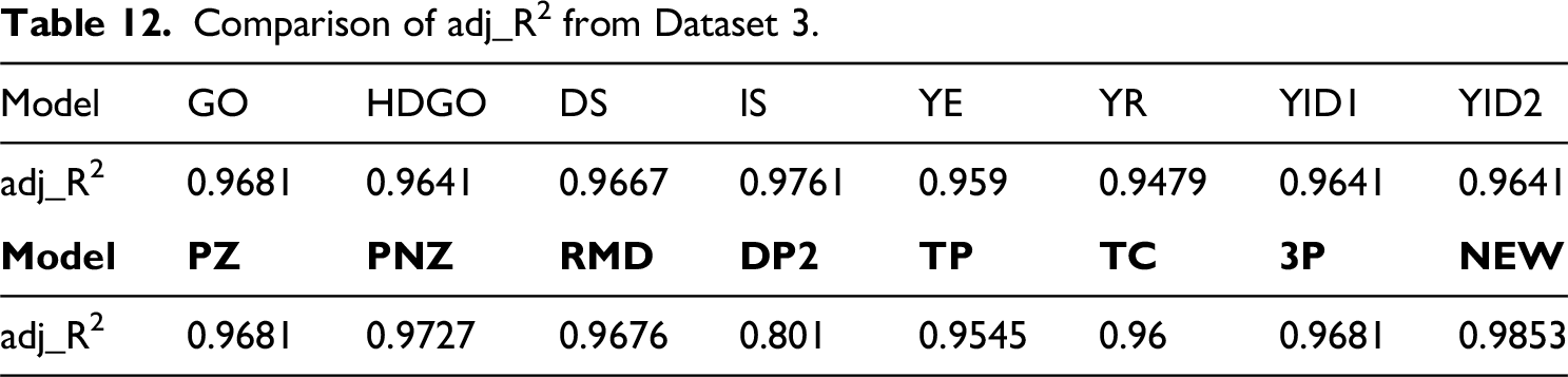
Tables 11 and 12 list the results of calculating nine criteria for the 16 models. Similar to Dataset 2, the MSE, MAE, PRR, PP, PRV, TS, AIC, and BIC were 15.2098, 4.2097, 0.081, 0.0701, 3.3235, 4.2571, 83.004, and 84.94, respectively. These values were close to zero. The value of adj_R² was 0.9853, which was the closest to 1. Among the 16 models tested, the proposed model exhibited the best results. This study improved the model and achieved superior results. Figure 9 compares the normalized metric-based models on Dataset 3 and shows that the new model performed better overall.

Figure 9.

Comparison of models based on normalized metrics for Dataset 3.

Table 11.

Comparison of criteria from Dataset 3.

Model	MSE	MAE	PRR	PP	PRV	TS	AIC	BIC
GO	33.9176	5.7228	0.2701	0.2246	5.5510	7.1075	92.7596	93.74
HDGO	37.6862	6.3587	0.2701	0.2246	5.5510	7.1075	94.7596	96.2143
DS	35.3906	4.9919	7.4621	0.7056	5.5277	7.2602	106.0925	107.0623
IS	25.1090	5.04	1.02	0.3332	4.4905	5.8015	91.4418	92.8966
YE	42.4210	7.1554	0.2700	0.2245	5.5526	7.1095	96.7692	98.7089
YR	53.8942	6.3821	18.9212	0.9323	5.9683	8.0134	118.4389	120.3785
YID1	37.7371	6.3628	0.2699	0.2245	5.5548	7.1123	94.7836	96.2383
YID2	37.6863	6.3587	0.2701	0.2246	5.5510	7.1075	94.7596	96.2144
PZ	32.2830	6.4663	1.02	0.3332	4.4904	5.8015	95.4418	97.8664
PNZ	28.2839	5.6509	1.0350	0.3337	4.4804	5.8052	93.4502	95.3898
RMD	33.5358	6.5326	0.8796	0.3258	4.9221	6.3212	96.1909	98.1305
DP2	205.8361	15.4728	0.6121	1.2264	12.2349	15.6606	141.8646	143.8043
TP	43.0042	8.8647	0.8600	0.3033	4.3859	5.6590	98.8173	102.2116
TC	40.5240	7.4735	1.5184	0.4075	5.0449	6.4999	101.0223	103.4469
3P	32.15	6.4694	1.0289	0.3332	4.4911	5.8022	95.4430	97.8675
NEW	15.2098	4.2097	0.0810	0.0701	3.3235	4.2571	83.0004	84.9400

Table 12.

Comparison of adj_R² from Dataset 3.

Model	GO	HDGO	DS	IS	YE	YR	YID1	YID2
adj_R²	0.9681	0.9641	0.9667	0.9761	0.959	0.9479	0.9641	0.9641
Model	PZ	PNZ	RMD	DP2	TP	TC	3P	NEW
adj_R²	0.9681	0.9727	0.9676	0.801	0.9545	0.96	0.9681	0.9853

Conclusion

Advancements in software have made it an integral part of our daily lives. The importance of software, ranging from very small tasks to the management and operation of entire systems, will become more critical with each passing day. Consequently, software reliability is of paramount importance, and considerable research has been conducted to improve it. This study proposes a model for enhancing software reliability. The proposed model reflects the potential for failures arising from increasingly complex software structures, and considers realistic scenarios. To address the potential for failure in complex software structures, the model considers both independent and dependent failures. To reflect a real environment, it was assumed that a certain degree of initial failure existed during the testing and operational stages. The superiority of the proposed model was demonstrated through three datasets using nine criteria, which yielded the best results. Note that it performed better than previous models, which assumed that the observation point was the initial point. By including the assumption of dependent failures, we created a model suitable for realistic situations. As dependence on software continues to increase, the importance of software also increases significantly. Consequently, research on software reliability models to enhance software reliability is expected to increase in importance. Therefore, we aim to extend the assumptions of this study to a software reliability model that can effectively address specific situations. This extension will incorporate assumptions such as changes in failure detection rates based on software time dependency, imperfect debugging, and operating environment uncertainty.

Footnotes

Acknowledgments

The authors would like to thank the National Research Foundation of Korea and CSU G-LAMP Project Group for their valuable support in this work.

ORCID iD

Kwang Yoon Song

Author contributions

Chang, I. H. and Pham, H conceived and designed the study; Song, K. Y. and Kim, Y. S. collected the data; Song, K. Y. and Kim, Y. S. performed the data analysis; Kim, Y. S. contributed to data interpretation; Song, K. Y. contributed to visualization; Song, K. Y. and Kim, Y. S. drafted the initial manuscript; Song, K, Y., Chang, I. H., and Pham, H. revised the manuscript critically for important intellectual content; and Chang, I. H. supervised the overall research process and managed the project. All authors read and approved the final version of the manuscript.

Funding

The authors disclosed receipt of the following financial support for the research, authorship, and/or publication of this article: This work was supported by the Global-Learning and Academic Research Institution for Master's and PhD students and the Postdoctoral Program of the National Research Foundation of Korea funded by the Ministry of Education (Grant No. RS-2023-00285353).

Declaration of conflicting interests

The authors declared no potential conflicts of interest with respect to the research, authorship, and/or publication of this article.

Data availability

The datasets generated and/or analyzed the current study are not publicly available bur are available from the corresponding author on reasonable request.

References

Kabanov

Madnick

. A systematic study of the control failures in the Equifax cybersecurity incident. MIT Sloan Research Paper, no. 2020-19, 2020. 2020.

Kabanov

Madnick

. Applying the lessons from the Equifax cybersecurity incident to build a better defense. MIS Q. Executive 2021; 20: 4.

Kim

Sohn

, et al. Time series analysis of groundwater level data obtained from national groundwater monitoring stations. Journal of the Geological Society of Korea 2004; 40: 305–329.

Jelinski

Moranda

. Software reliability research. In: Statistical computer performance evaluation. New York, NY, USA: Academic Press, 1972, pp.465–484.

Goel

Okumoto

. Time-dependent error-detection rate model for software reliability and other performance measures. IEEE Trans. Reliab 1979; 28: 206–211.

Ohishi

Okamura

Dohi

. Gompertz software reliability model: estimation algorithm and empirical validation. J Syst Softw 2009; 82: 535–543.

Musa

. The measurement and management of software reliability. Proc IEEE 2005; 68: 1131–1143.

Pham

Zhang

. NHPP software reliability and cost models with testing coverage. Eur J Oper Res 2003; 145: 443–454.

Yamada

Tokuno

Osaki

. Imperfect debugging models with fault introduction rate for software reliability assessment. Int J Syst Sci 1992; 23: 2241–2252.

10.

Yamada

Ohtera

Narihisa

. A testing-effort dependent software reliability model and its application. Microelectron Reliab 1987; 27: 507–522.

11.

Huang

Lin

. Software reliability analysis by considering fault dependency and debugging time lag. IEEE Trans Reliab 2006; 55: 436–450.

12.

Pham

. An imperfect-debugging fault-detection dependent-parameter software. Int J Autom Comput 2007; 4: 325–328.

13.

Barlow

Marshall

. Bounds for distributions with monotone hazard rate, I. The Annals of Mathematical Statistics 1964; 35: 1234–1257.

14.

Barlow

Marshall

. Bounds for distributions with monotone hazard rate, II. The Annals of Mathematical Statistics 1964; 35: 1258–1274.

15.

Hossain

Dahiya

. Estimating the parameters of a non-homogeneous Poisson-process model for software reliability. IEEE Trans Reliab 1993; 42: 604–612.

16.

Yamada

Ohba

Osaki

. S-shaped reliability growth modeling for software fault detection. IEEE Trans. Reliab 1983; 32: 475–484.

17.

M. Inflection S-shaped software reliability growth model. In Stochastic models in reliability theory; Osaki S and Hatoyama Y (Eds). Springer: Berlin, Germany, 1984; pp. 144–162.

18.

Yamada

Ohtera

Narihisa

. Software reliability growth models with testing-effort. IEEE Trans. Reliab 1986; 35: 19–23.

19.

Huang

Kuo

Lyu

. An assessment of testing-effort dependent software reliability growth models. IEEE Trans Reliab 2007; 56: 198–211.

20.

Peng

Zhang

, et al. Testing effort dependent software reliability model for imperfect debugging process considering both detection and correction. Reliab Eng Syst Saf 2014; 126: 37–43.

21.

Yamada

Tokuno

Osaki

. Imperfect debugging models with fault introduction rate for software reliability assessment. Int. J. Syst. Sci 1992; 23: 2241–2252.

22.

Pham

Zhang

. An NHPP software reliability models and its comparison. Int. J. Reliab. Qual. Saf. Eng 1997; 4: 269–282.

23.

Pham

Nordmann

Zhang

. A general imperfect software debugging model with S-shaped fault detection rate. IEEE Trans. Reliab 1999; 48: 169–175.

24.

Roy

Mahapatra

Dey

. An NHPP software reliability growth model with imperfect debugging and error generation. Int. J. Reliab. Qual. Saf. Eng 2014; 21: 1–3.

25.

Teng

Pham

. A new methodology for predicting software reliability in the random field environments. IEEE Trans. Reliab 2006; 55: 458–468.

26.

Honda

Washizaki

Fukazawa

. Generalized software reliability model considering uncertainty and dynamics: model and applications. Int J Software Engineer Knowledge Engineer 2017; 27: 967–993.

27.

Asraful Haque

Ahmad

. A logistic growth model for software reliability estimation considering uncertain factors. Int J Reliab Qual Saf Eng 2021; 28: 2150032.

28.

Chang

Pham

Lee

, et al. A testing-coverage software reliability model with the uncertainty of operation environments. Int. J. Syst. Sci.-Oper. Logist 2014; 1: 220–227.

29.

Song

Chang

Pham

. A three-parameter fault-detection software reliability model with the uncertainty of operating environments. J. Syst. Sci. Syst. Eng 2017; 26: 121–132.

30.

Chatterjee

Saha

Sharma

. Multi-upgradation software reliability growth model with dependency of faults under change point and imperfect debugging. Journal of Software: Evolution and Process 2021; 33: e2344.

31.

Samal

Kumar

. Redefining software reliability modeling: embracing fault-dependency, imperfect removal, and maximum fault considerations. Qual Eng 2024; 36: 500–509.

32.

Hussain

Oraibi

Mashikhin

, et al. New software reliability growth model: piratical swarm optimization-based parameter estimation in environments with uncertainty and dependent failures. Statistics, Optimization & Information Computing 2025; 13: 209–221.

33.

Crow

. Reliability analysis for complex, repairable systems (No. AMSAATR138). 1975.

34.

Pan

Nonaka

. Importance analysis for the systems with common cause failures. Reliab. Eng. Syst. Saf 1995; 50: 297–300.

35.

Pham

. Software reliability models with time dependent hazard rate based on Bayesian approach. IEEE Trans. Syst. Man Cybern. Part A-Syst. Hum 2000; 30: 25–35.

36.

Zhang

Jeske

Pham

. Calibrating software reliability models when the test environment does not match the user environment. Appl Stoch Models Bus Ind 2002; 18: 87–99.

37.

Chandrika

. Study on software reliability and reliability testing. Asia-pacific Journal of Convergent Research Interchange 2015; 1: 7–20.

38.

Armstrong

Collopy

. Error measures for generalizing about forecasting methods: empirical comparisons. Int. J. Forecast 1992; 8: 69–80.

39.

Willmott

Matsuura

. Advantages of the mean absolute error (MAE) over the root mean square error (RMSE) in assessing average model performance. Clim. Res 2005; 30: 79–82.

40.

Iqbal

. Software reliability growth models: a comparison of linear and exponential fault content functions for study of imperfect debugging situations. Cogent Eng 2017; 4: 1286739.

41.

Pillai

Nair

. A model for software development effort and cost estimation. IEEE Trans. Softw. Eng 1997; 23: 485–497.

42.

Sharma

Garg

Nagpal

, et al. Selection of optimal software reliability growth models using a distance based approach. IEEE Trans. Reliab 2010; 59: 266–276.

43.

Kuha

. AIC and BIC: comparisons of assumptions and performance. Sociol. Methods Res 2004; 33: 188–229.

44.

Jeske

Zhang

. Some successful approaches to software reliability modeling in industry. J. Syst. Softw 2005; 74: 85–99.

45.

Wang

Liu

. Software reliability growth modeling and analysis with dual fault detection and correction processes. IIE Trans 2016; 48: 359–370.

Nonhomogeneous Poisson process software reliability model incorporating initial fault diversification and dependent failures

Abstract

Keywords

Introduction

Related research for software reliability model

A new software reliability model

Dependent failure software reliability model

Proposed dependent failure software reliability model

Numerical examples

Data introduction

Criteria

Analysis results

Analysis results for Dataset 1

Analysis results for Dataset 2

Analysis results for Dataset 3

Conclusion

Footnotes

Acknowledgments

ORCID iD

Author contributions

Funding

Declaration of conflicting interests

Data availability

References