Isogeometric boundary element method analysis for dielectric target shape optimization in electromagnetic scattering

Abstract

In order to optimize the overall form of electromagnetic scattering in two-dimensional dielectric media, this work offers a frequency-domain boundary element method based on isogeometric analysis. The Isogeometric boundary element method (IGABEM) is used to guarantee geometric correctness during optimization and prevent over-refinement of the mesh. Non-uniform rational B-splines are used to discretize the boundary integrals of the model, enabling rapid numerical computation while ensuring high accuracy. Furthermore, as an alternative model for electromagnetic scattering shape optimization issues, a gray wolf optimizer-based back-propagation neural network (GWO-ANN) is created, with radar cross-section (RCS) as the objective function. Finally, the GWO-ANN is used as a surrogate model for shape optimization in multi-frequency electromagnetic scattering problems with the RCS as the objective function. In computational examples, this algorithm efficiently and accurately solves electromagnetic scattering problems under multiple frequencies.

Introduction

Electromagnetic simulation of complex targets has significant applications in engineering and biomedical field. For example, it is applied to the analysis and design of microwave circuits and to radiofrequency ablation, nerve stimulation, and ultrasonic imaging.^1–3 In electromagnetic scattering analysis, differential equation methods are primarily used, including the finite element method (FEM)^4–6 and the time-domain finite difference method (TD-FDM).^7,8

The boundary element method (BEM), also called the method of moment (MoM) in computational electromagnetics, stands as a widely utilized technique in computational electromagnetics.^9–13 The original physical problem was mathematically changed by Maao ¹⁴ to have propagation velocities with reduced frequency dependency. A unique hybrid boundary element-finite element system was presented by Ren et al. ¹⁵ to model three-dimensional (3D) plane wave electromagnetic reactions in the earth. These approaches necessitate domain meshing, resulting in notable mesh truncation and dispersion errors. Additionally, accurately conforming to the complex target surface presents a challenging task. Thus, the calculation error is not controllable. Precise calculations may be obtained by introducing the fundamental solutions of differential equations and developing surface integral equations using the vector BEM. Besides, for problems in infinite domains, the Sommerfeld radiation condition is automatically met when solved numerically using BEM. ¹⁶ Additionally, traditional BEM cannot be used for large-scale problems because the coefficient matrices formed are dense matrices with high memory requirements. Fortunately, although dense, the boundary element coefficient matrix possesses the property of low-rank partitioning. There are a series of fast methods utilizing low-rank decomposition, including the fast multipole method,^17,18 etc., which have successfully reduced computational complexity and memory usage. These fast methods enable the application of BEM to complex engineering problems.^19,20

Traditional BEM uses Lagrange functions as basis functions, such as Raviart–Thomas ²¹ and Rao–Wilton–Glisson (RWG) ²² basis functions, primarily relying on low-order polynomials. The majority of traditional numerical techniques use RWG or Raviart–Thomas basis functions, which are derived from low-order polynomials. Advances in isogeometric analysis (IGA) have promoted the development of spline-based consistent discretization, which makes it possible to construct discrete de Rham sequences. ²³ This advancement represents a significant stride toward utilizing IGA in fluid flow or electromagnetic applications. In the shape optimization (SO) process, there are several challenges: (a) Capturing complex details of intricate structures is very difficult; inaccurate capturing may affect geometric precision. Approximating the physical field with low-order basis functions can reduce the precision and sensitivity analysis of the target. (b) The structure’s shape changes with variations in shape variables, requiring the grid to be redefined at each iteration, leading to significant time waste. (c) To achieve large-scale shape variations, a significant amount of shape variable data must be input during the optimization calculations. Nevertheless, this method may result in significant computational expenses and difficulties guaranteeing that the structure transforms into the intended shape.^24,25 Hughes proposed IGA, ²⁶ which is a new numerical computation technique based on spline theory. IGA was widely used as soon as it was proposed.^27–34 IGA makes the acoustic boundary element simulation computation easier, more accurate, and more precise. The method can be used to analyze the computer-aided design (CAD) model directly without additional meshing, which reduces the discretization error of the model and speeds up the computation.^35,36 Non-uniform rational b-splines (NURBS) ³⁷ and t-splines are used instead^38–40 of traditional finite elements. Without changing the geometry, we can improve the accuracy of the simulation by h- and p-refinement. To facilitate a more general geometric representation in design, IGA integrates t-splines characterized by t-joints, which can be locally optimized in the analysis. Surface subdivision is an effective surface design technique with a simple refinement process that effectively generates smooth surfaces from any original mesh. Buffa et al. ²³ proposed vector field-oriented FEM based on B-spline volumetric shape functions suitable for non-uniform media. Simpson et al. ⁴¹ introduced IGA into BEM and developed a vector field-oriented IGABEM for electromagnetic scattering analysis of pure metal structures. Vector field-oriented IGABEM was applied by Takahashi et al.^42,43 to tackle the electromagnetic scattering issue of 3D doubly periodic multilayer structures. In this study, NURBS–IGABEM is used to improve the calculation accuracy for dielectric (DIE) targets in electromagnetic scattering problems.

The SO technique realizes radar stealth^44,45 by changing the original shape of the object and reducing the radar cross-section (RCS) of the object. ⁴⁶ Fundamentally, the SO method propels the transformation of geometric models into their optimal states by facilitating seamless information exchange between computer-aided engineering and CAD. ⁴⁷ Firstly, the objective function, design variables, and constraint conditions are set. Secondly, a numerical analysis is employed to solve the objective function along with its shape sensitivity. Finally, the design variables are automatically updated with optimization operators to realize the shape evolution of the structure. Nowadays, Isogeometric methods have been successfully applied to SO in a number of fields.^48–56 SO was advanced in the field of electromagnetic by Takahashi et al., ⁵⁷ who created a 3D SO framework for the wave equation based on time-domain BEM. The particle swarm optimization algorithm is used to handle form and size optimization challenges in instructional design by Fourie and Groenwold, ⁵⁸ which provided a new method for SO. However, there is presently no documented report specifically focusing on SO utilizing IGA within the realm of electromagnetic fields. ⁵³ In this work, the use of the NURBS-based IGA modeling method reduces the dimensionality of the design variables, making the model’s shape smoother and more flexible.

This study’s goal is to investigate the use of IGABEM for multi-frequency electromagnetic scattering SO. This is an area of research that has not received much attention in the literature so far. The innovations of this paper include the following points:

IGABEM is employed for the electromagnetic scattering analysis of DIE targets, with a comprehensive investigation into the impacts of DIE constant, frequency, and incident wave on the scattering field.

The SO approach with IGABEM is introduced for DIE electromagnetics.

The remainder of this article is organized as follows: Section “Solution of objective function based on IGABEM” introduces IGABEM for solving the objective function of electromagnetic scattering. Section “Optimization analysis for electromagnetic scattering based on deep learning” enhances the algorithm’s learning and prediction capabilities through the gray wolf optimization (GWO) algorithm. Numerical examples are provided in Sections “Numerical examples—IGABEM for electromagnetic scattering” and“Numerical examples—SO for electromagnetic scattering” to support the suggested optimization procedure. Section “Conclusions” concludes the findings of thisstudy.

Solution of objective function based on IGABEM

In this section, the surface integral equations were solved using IGABEM to obtain initial data, from which surface currents were derived. Integrating the two-dimensional electric^59–61 radiation equation with these surface currents, the scattering field is derived. The scattering field and incident field are combined to obtain the two-dimensional RCS value of the objective function.

Surface integral equation

Assume the DIE region ${\mathrm{\Omega }}_1$ , with its closed boundary $\mathrm{\Gamma }$ located within the infinite domain ${\mathrm{\Omega }}_0$ , where the DIE constant and magnetic permeability of the infinite domain are defined by ${\epsilon }_0$ and ${\mu }_0$ , respectively. Additionally, we assume the presence of a polarized harmonic electromagnetic plane wave ${\mathbf{E}}_{\text{inc}}$ propagating through the DIE region at an angular frequency of $\omega$ , with a wave number of $k=\omega \sqrt{{\epsilon }_0{\mu }_0}$ . The scenario is illustrated in Figure 1. The surface integral equation for ${\mathrm{\Omega }}_l$ with $l=0,1$ is given by:

$$\begin{array}{rl}{\left[{\mathbf{E}}_{\text{inc}}^l(\tilde{\mathbf{r}})\right]}_{\tan }& =\frac{1}{2}{\hat{\mathbf{n}}}^l(\tilde{\mathbf{r}})\times {\mathbf{M}}^l(\tilde{\mathbf{r}})\\ & +{\left[\text{i}\omega {\mu }^l(\mathcal{L}{\mathbf{J}}^l)(\tilde{\mathbf{r}})+(\mathcal{K}{\mathbf{M}}^l)(\tilde{\mathbf{r}})\right]}_{\tan }\\ {\hat{\mathbf{n}}}^l(\tilde{\mathbf{r}})\times {\left[{\mathbf{H}}_{\mathrm{inc}}^l(\tilde{\mathbf{r}})\right]}_{\tan }& =\frac{1}{2}{\mathbf{J}}^l(\tilde{\mathbf{r}})\end{array}$$

(1)

$$-{\hat{\mathbf{n}}}^l(\tilde{\mathbf{r}})\times {\left[\mathrm{i}\omega {\epsilon }^l(\mathcal{L}{\mathbf{M}}^l)(\tilde{\mathbf{r}})-(\mathcal{K}{\mathbf{J}}^l)(\tilde{\mathbf{r}})\right]}_{\tan }$$

(2)

where the operators $\mathcal{L}$ and $\mathcal{K}$ are

$$\begin{array}{cc}& \left(\mathcal{L}{\mathbf{J}}^l\right)\left(\tilde{\mathbf{r}}\right)=\left[1+\frac{1}{k^2}\mathrm{\nabla }\mathrm{\nabla }\cdot \right]{\displaystyle {\int }_{{\mathrm{\Gamma }}^l(\mathbf{r})}^{G\left(\tilde{\mathbf{r}},\mathbf{r}\right){\mathbf{J}}^l\left(\mathbf{r}\right)d{\mathrm{\Gamma }}^l(\mathbf{r}})}\\ & \left(\mathcal{K}{\mathbf{M}}^l\right)\left(\tilde{\mathbf{r}}\right)=\mathrm{\nabla }\times {\displaystyle {\int }_{{\mathrm{\Gamma }}^l(\mathbf{r})}^{G\left(\tilde{\mathbf{r}},\mathbf{r}\right){\mathbf{M}}^l\left(\mathbf{r}\right)d{\mathrm{\Gamma }}^l(\mathbf{r}})}\end{array}$$

(3)

Here, ${\mathbf{E}}_{\text{inc}}^l(\tilde{\mathbf{r}})$ represent the electric field and ${\mathbf{H}}_{\text{inc}}^l(\tilde{\mathbf{r}})$ represent the magnetic field that the incoming wave produces, which equal zero outside ${\mathrm{\Omega }}_0$ . $G(\tilde{\mathbf{r}},\mathbf{r})$ is Green’s function. In the two-dimensional problem:

$$G\left(\tilde{\mathbf{r}},\mathbf{r}\right)=-\frac{\text{i}}{4}{H}_0^{\left(2\right)}\left(kr\right),\text{with}r=|\tilde{\mathbf{r}}-\mathbf{r}|$$

(4)

Equation (1) represents the electric field integral equation (EFIE)^62–64 and equation (2) represents the non-uniform magnetic field integral equation (nMFIE). Calculating equations (1) and (2) for DIE materials does not lead to spurious solutions. Therefore, it can be directly used in the calculation of DIE electromagnetic scattering.

Figure 1.

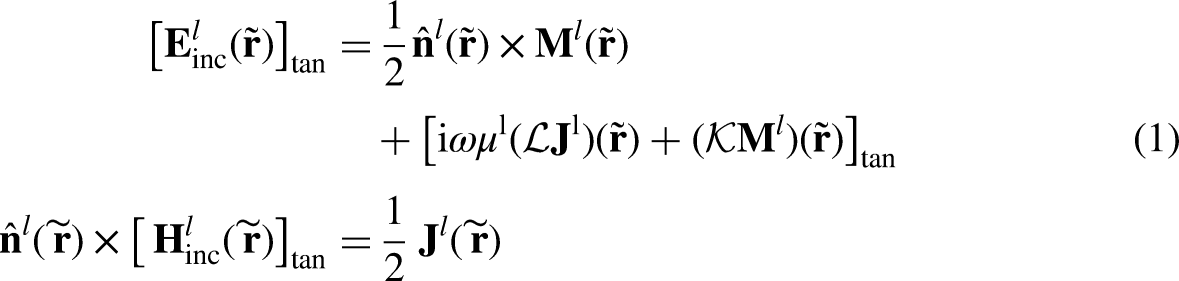
Plane wave: The infinite domain ${\mathrm{\Omega }}_0$ assigns the parameters $({\mu }_0,{\epsilon }_0)$ of free space; $\mathrm{\Gamma }$ denotes the boundary of dielectric target ${\mathrm{\Omega }}_1$ with parameters $({\mu }_1,{\epsilon }_1)$ . On the boundary, the normal vector ${\hat{\mathbf{n}}}^1$ points into ${\mathrm{\Omega }}_1$ .

Discretization of BEM based on NURBS

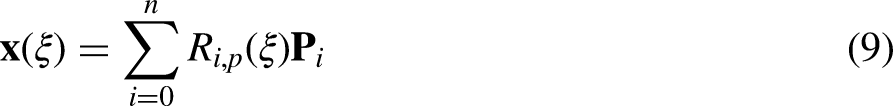
The NURBS curve ⁶⁵ is defined by a knot vector, which refers to a set of non-decreasing real numbers specified in the parameter space. Generally, the knot vector is denoted by $\mathrm{\Xi }=[{\xi }_0,{\xi }_1,\dots ,{\xi }_m]$ , where ${\xi }_i\in \mathbf{R}$ . We assume the length of the knot vector to be $m=n+p+1$ , where $p$ represents the polynomial degree and $n$ represents the number of basis functions or control points. The recursive expression for the B-spline basis function $N_{i,p}$ is:

$$N_{i,0}(\xi )=\{\begin{array}{cc}& 1\mathrm{if}{\xi }_i\le \xi <{\xi }_{i+1}\\ & 0\mathrm{otherwise}\end{array}$$

(5)

and for $p=1,2,3,\dots$

$$\begin{array}{rl}{N}_{i,p}(\xi )& =\frac{\xi -{\xi }_i}{{\xi }_{i+p}-{\xi }_i}{N}_{i,p-1}(\xi )\\ & +\frac{{\xi }_{i+p+1}-\xi }{{\xi }_{i+p+1}-{\xi }_{i+1}}{N}_{i+1,p-1}(\xi )\end{array}$$

(6)

B-spline basis functions possess characteristics such as continuity and efficiency. NURBS extend B-splines where control points are weighted as:

$$R_{i,p}(\xi )=\frac{N_{i,p}(\xi )w_i}{W(\xi )}$$

(7)

with

$$W(\xi )=\sum _{i=0}^n{w}_i{N}_{i,p}(\xi )$$

(8)

In equation (7), $R_{i,p}(\xi )$ represents the NURBS basis function, and $w_i$ denotes the weight associated with the control points. The NURBS curve point $\mathbf{x}(\xi )$ can then be expressed as:

$$\mathbf{x}(\xi )=\sum _{i=0}^n{R}_{i,p}(\xi ){\mathbf{P}}_i$$

(9)

where ${\mathbf{P}}_i$ denotes the $i$ th control point.

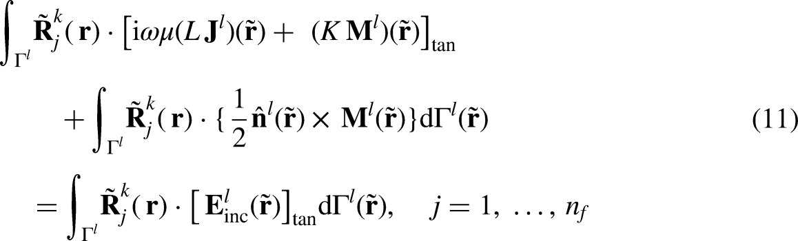
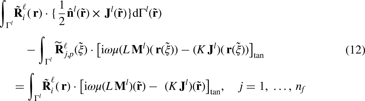
Using isogeometric BEM, the current and magnetic flow in ${\mathrm{\Omega }}_l$ in equation (1) can be converted to the summation form of NURBS basis functions:

$$\begin{array}{cc}& {\mathbf{J}}^l\left(\mathbf{r}\right)={\displaystyle \sum _{i=1}^{N_f}{\mathbf{R}}_i^k\left(\mathbf{r}\right)X_i^J}\\ & {\mathbf{M}}^l\left(\mathbf{r}\right)={\displaystyle \sum _{i=1}^{N_f}{\mathbf{R}}_i^{\ell }\left(\mathbf{r}\right)X_i^M}\end{array}$$

(10)

The terms ${\mathbf{R}}_i^k(\tilde{\mathbf{r}})=R_i^{(}\tilde{\mathbf{r}})\hat{\mathbf{k}}$ and ${\mathbf{R}}_i^{\ell }(\mathbf{r})=R_i^{(}\mathbf{r})\hat{\mathbf{e}}$ , respectively, represent the $\hat{\kappa }$ -direction current and $\hat{\ell }$ -direction magnetic flux; $\tilde{\mathbf{r}}=\tilde{\mathbf{r}}(\xi )$ ; $X_i^J$ and $X_i^M$ , respectively, denote the global parameters of current and magnetic flux inside ${\mathrm{\Omega }}_l$ connected to the control point $i$ th; $N$ denotes the control points’ total number. Taking into account the directional nature of surface currents, the B-spline approximation mentioned in Simpson et al. ⁴¹ is used to represent surface currents.

In electromagnetic problems, BEM is commonly known as the MoMs. Similar to Galerkin BEM, it employs basis functions as test functions and has the characteristic of enforced boundary conditions across the entire solution. In our case, we will use the electric test functions ${\tilde{\mathbf{r}}}_i^k(\tilde{\mathbf{r}})=R_i^{(}\tilde{\mathbf{r}})\hat{\mathbf{k}}$ and ${\tilde{\mathbf{r}}}_i^{\ell }(\mathbf{r})=R_i^{(}\mathbf{r})\hat{\mathbf{e}}$ to test the EFIE and nMFIE. This operation results in

$$\begin{array}{rl}& {\int }_{{\mathrm{\Gamma }}^l}{\tilde{\mathbf{R}}}_j^k(\mathbf{r})\cdot {\left[\mathrm{i}\omega \mu (L{\mathbf{J}}^l)(\tilde{\mathbf{r}})+(K{\mathbf{M}}^l)(\tilde{\mathbf{r}})\right]}_{\tan }\\ & +{\int }_{{\mathrm{\Gamma }}^l}{\tilde{\mathbf{R}}}_j^k(\mathbf{r})\cdot \{\frac{1}{2}{\hat{\mathbf{n}}}^l(\tilde{\mathbf{r}})\times {\mathbf{M}}^l(\tilde{\mathbf{r}})\}\mathrm{d}{\mathrm{\Gamma }}^l(\tilde{\mathbf{r}})\\ & ={\int }_{{\mathrm{\Gamma }}^l}{\tilde{\mathbf{R}}}_j^k\left(\mathbf{r}\right)\cdot {\left[{\mathbf{E}}_{\mathrm{inc}}^l(\tilde{\mathbf{r}})\right]}_{\tan }\mathrm{d}{\mathrm{\Gamma }}^l(\tilde{\mathbf{r}}),j=1,\dots ,n_f\end{array}$$

(11)

and

$$\begin{array}{rl}& {\int }_{{\mathrm{\Gamma }}^l}{\tilde{\mathbf{R}}}_i^{\ell }(\mathbf{r})\cdot \{\frac{1}{2}{\hat{\mathbf{n}}}^l(\tilde{\mathbf{r}})\times {\mathbf{J}}^l(\tilde{\mathbf{r}})\}\mathrm{d}{\mathrm{\Gamma }}^l(\tilde{\mathbf{r}})\\ & -{\int }_{{\mathrm{\Gamma }}^l}{\tilde{\mathbf{R}}}_{j,p}^{\ell }(\tilde{\xi })\cdot {\left[\mathrm{i}\omega \mu (L{\mathbf{M}}^l)(\mathbf{r}(\tilde{\xi }))-(K{\mathbf{J}}^l)(\mathbf{r}(\tilde{\xi }))\right]}_{\tan }\\ & ={\int }_{{\mathrm{\Gamma }}^l}{\tilde{\mathbf{R}}}_i^{\ell }(\mathbf{r})\cdot {\left[\mathrm{i}\omega \mu (L{\mathbf{M}}^l)(\tilde{\mathbf{r}})-(K{\mathbf{J}}^l)(\tilde{\mathbf{r}})\right]}_{\tan },j=1,\dots ,n_f\end{array}$$

(12)

The matrix form of IGABEM is derived as equation (13) by substituting equation (10) into equations (11) and (12):

$$\left[\begin{array}{cc}{A}_E^J& A_E^M\\ A_H^J& A_H^M\end{array}\right]\left[\begin{array}{c}{X}^J\\ X^M\end{array}\right]=\left[\begin{array}{c}{B}_E^l\\ B_H^l\end{array}\right]$$

(13)

with the matrix elements given by

$$\begin{array}{rl}{A}_E^J(j,i)& =\mathrm{i}\omega {\mu }^l\sum _{\tilde{e}=1}^{N_e}\sum _{e=1}^{N_e}{\int }_{{\xi }_{\tilde{e}}}^{{\xi }_{\tilde{e}+1}}{\tilde{\mathbf{R}}}_j^{\kappa }(\mathbf{r})\\ & \cdot {\int }_{{\xi }_e}^{{\xi }_{e+1}}{\mathbf{R}}_i^k(\tilde{\mathbf{r}})G(\tilde{\mathbf{r}},\mathbf{r})\mathrm{d}{\mathrm{\Gamma }}^l(\mathbf{r})\mathrm{d}{\mathrm{\Gamma }}^l(\tilde{\mathbf{r}})\\ & +\frac{\mathrm{i}}{\omega {\epsilon }^l}\sum _{\tilde{e}=1}^{N_e}\sum _{e=1}^{N_e}{\int }_{{\xi }_{\tilde{e}}}^{{\xi }_{\tilde{e}+1}}{\mathbf{R}}_i^k(\tilde{\mathbf{r}})\cdot [\mathrm{\nabla }\mathrm{\nabla }\\ (14)& & \cdot {\int }_{{\xi }_e}^{{\xi }_{e+1}}{\mathbf{R}}_i^k(\tilde{\mathbf{r}})G(\tilde{\mathbf{r}},\mathbf{r})\mathrm{d}{\mathrm{\Gamma }}^l(\tilde{\mathbf{r}})]\mathrm{d}{\mathrm{\Gamma }}^l(\tilde{\mathbf{r}})A_E^M(j,i)& =\sum _{\tilde{e}=1}^{N_e}\sum _{e=1}^{N_e}{\int }_{{\xi }_{\tilde{e}}}^{{\xi }_{\tilde{e}+1}}{\tilde{\mathbf{r}}}_j^k\left(\mathbf{r}\right)\cdot {\int }_{{\xi }_e}^{{\xi }_{e+1}}\mathrm{\nabla }G(\tilde{\mathbf{r}},\mathbf{r})\\ & \times {\mathbf{R}}_i^{\ell }(\tilde{\mathbf{r}})\mathrm{d}{\mathrm{\Gamma }}^l(\tilde{\mathbf{r}})\mathrm{d}{\mathrm{\Gamma }}^l(\mathbf{r})+\frac{1}{2}\sum _{\tilde{e}=1}^{N_e}{\int }_{{\xi }_{\tilde{e}}}^{{\xi }_{\tilde{e}+1}}{\tilde{\mathbf{R}}}_j^k\left(\mathbf{r}\right)\\ (15)& & \cdot [\hat{\mathbf{n}}(\mathbf{r})\times {\tilde{\mathbf{R}}}_i^{\ell }(\mathbf{r})]\mathrm{d}{\mathrm{\Gamma }}^l(\tilde{\mathbf{r}})A_H^J(j,i)& =-\sum _{\tilde{e}=1}^{N_e}\sum _{e=1}^{N_e}{\int }_{{\xi }_{\tilde{e}}}^{{\xi }_{\tilde{e}+1}}{\tilde{\mathbf{R}}}_i^{\ell }(\mathbf{r})\\ & \cdot {\int }_{{\xi }_e}^{{\xi }_{e+1}}\mathrm{\nabla }G(\tilde{\mathbf{r}},\mathbf{r})\times {\mathbf{R}}_i^k(\tilde{\mathbf{r}})\mathrm{d}{\mathrm{\Gamma }}^l(\tilde{\mathbf{r}})\mathrm{d}{\mathrm{\Gamma }}^l(\mathbf{r})\\ & -\frac{1}{2}\sum _{\tilde{e}=1}^{N_e}{\int }_{{\xi }_{\tilde{e}}}^{{\xi }_{\tilde{e}+1}}{\tilde{\mathbf{R}}}_i^{\ell }(\mathbf{r})\cdot [\hat{\mathbf{n}}(\mathbf{r})\\ (16)& & \times {\mathbf{R}}_i^k(\tilde{\mathbf{r}})]\mathrm{d}{\mathrm{\Gamma }}^l(\tilde{\mathbf{r}})A_H^M(j,i)& =\mathrm{i}\omega {\epsilon }^l\sum _{\tilde{e}=1}^{N_e}\sum _{e=1}^{N_e}{\int }_{{\xi }_{\tilde{e}}}^{{\xi }_{\tilde{e}+1}}{\tilde{\mathbf{R}}}_i^{\ell }(\mathbf{r})\\ & \cdot {\int }_{{\xi }_e}^{{\xi }_{e+1}}{\mathbf{R}}_i^{\ell }(\tilde{\mathbf{r}})G(\tilde{\mathbf{r}},\mathbf{r})\mathrm{d}{\mathrm{\Gamma }}^l(\mathbf{r})\mathrm{d}{\mathrm{\Gamma }}^l(\tilde{\mathbf{r}})\\ & +\frac{\mathrm{i}}{\omega {\epsilon }^l}\sum _{\tilde{e}=1}^{N_e}\sum _{e=1}^{N_e}{\int }_{{\xi }_{\tilde{e}}}^{{\xi }_{\tilde{e}+1}}{\tilde{\mathbf{R}}}_i^{\ell }(\mathbf{r})\cdot [\mathrm{\nabla }\mathrm{\nabla }\end{array}$$

$$\cdot {\int }_{{\xi }_e}^{{\xi }_{e+1}}{\tilde{\mathbf{R}}}_i^{\ell }(\mathbf{r})G(\tilde{\mathbf{r}},\mathbf{r})\mathrm{d}{\mathrm{\Gamma }}^l(\mathbf{r})]\mathrm{d}{\mathrm{\Gamma }}^l(\mathbf{r})$$

(17)

The right vector element of equation (13) could be expressed as:

$$B_E^l(j)=\sum _{\tilde{e}=1}^{N_e}{\int }_{{\xi }_{\tilde{e}}}^{{\xi }_{\tilde{e}+1}}{\tilde{\mathbf{R}}}_j^k\left(\mathbf{r}\right)\cdot {\mathbf{E}}_{\mathrm{inc}}^l(\tilde{\mathbf{r}})\mathrm{d}{\mathrm{\Gamma }}^l(\mathbf{r})$$

(18)

$$B_H^l(j)=\sum _{\tilde{e}=1}^{N_e}{\int }_{{\xi }_{\tilde{e}}}^{{\xi }_{\tilde{e}+1}}{\tilde{\mathbf{R}}}_i^{\ell }(\mathbf{r})\cdot {\mathbf{H}}_{\mathrm{inc}}^l(\tilde{\mathbf{r}})\mathrm{d}{\mathrm{\Gamma }}^l(\tilde{\mathbf{r}})$$

(19)

Using the above equations, the current and magnetic flux could be calculated.

Calculation of objective function

RCS measures the strength of the echo generated by a target when illuminated by radar waves. It is commonly used to assess the detectability of targets by radar systems. The calculation formula for RCS is:

$$\mathrm{RCS}{}_{2\mathrm{D}}=2\pi \rho \frac{|E_{\text{sca}}{|}^2}{|E_{\text{inc}}{|}^2}$$

(20)

where $\rho$ represents the distance between the source point and the field point. $E_{\text{inc}}$ represents the incident electric field. The $E_{\text{sca}}$ represents the electric strength of the scattered field. Under transverse electric (TE ) polarization, the incident electric field and incident magnetic field, respectively, are:

$$\begin{array}{rl}{\mathbf{E}}_{\mathrm{inc}}^l(\tilde{\mathbf{r}})& =e^{\mathrm{i}k\left(x_1\cos \left({\varphi }_{\mathrm{inc}}\right)+x_2\sin \left({\varphi }_{\mathrm{inc}}\right)\right)}\hat{\mathbf{z}}\\ {\mathbf{H}}_{\mathrm{inc}}^l\left(\tilde{\mathbf{r}}\right)& =\frac{1}{\eta }\left[-\sin \left({\varphi }_{\mathrm{inc}}\right)\widetilde{{\mathbf{r}}_1}+\cos \left({\varphi }_{\mathrm{inc}}\right)\widetilde{{\mathbf{r}}_2}\right]\end{array}$$

(21)

$$\cdot e^{\mathrm{i}k\left(x_1\cos \left({\varphi }_{\mathrm{inc}}\right)+x_2\sin \left({\varphi }_{\mathrm{inc}}\right)\right)}$$

(22)

Under transverse magnetic (TM) polarization, the incident electric field, and incident magnetic field, respectively, are:

$$\begin{array}{rl}{\mathbf{E}}_{\mathrm{inc}}^l(\tilde{\mathbf{r}})& =\left[{\tilde{\mathbf{r}}}_1\sin ({\varphi }^{\mathrm{inc}})-\cos ({\varphi }^{\mathrm{inc}}){\tilde{\mathbf{r}}}_2\right]\\ & \cdot e^{\mathrm{i}k\left(x\cos \left({\varphi }^{\mathrm{inc}}\right)+y\sin \left({\varphi }^{\mathrm{inc}}\right)\right)}\end{array}$$

(23)

$${\mathbf{H}}_{\mathrm{inc}}^l\left(\tilde{\mathbf{r}}\right)=\frac{1}{\eta }{e}^{\mathrm{i}k\left(x\cos \left({\varphi }_{\mathrm{inc}}\right)+y\sin \left({\varphi }_{\mathrm{inc}}\right)\right)}\hat{\mathbf{z}}$$

(24)

RCS is usually expressed as:

$$\mathrm{RCS}\left(\mathrm{dbsm}\right)=10\times \lg \mathrm{RCS}({\text{m}}^2)$$

(25)

The locations of the source and field points are connected to the bistatic RCS. The bistatic angle is the angle formed by the incident and the scattering wave, denoted by ${\varphi }^s$ . The electromagnetic scattering function $p(f)$ is frequency-dependent, and therefore the objective function $\mathrm{\Pi }$ is also frequency-dependent. As a result, optimization may only be applied at specific frequencies. The objective function is adjusted to fit the frequency band $[f_l,f_u]$ in order to resolve this problem:

$$\begin{array}{rl}{\mathrm{\Pi }}_{\mathrm{new}}& =\frac{1}{f_u-f_l}{\int }_{f_l}^{f_u}\mathrm{\Pi }(p\left(f\right))\mathrm{d}f\\ & \approx \frac{1}{f_u-f_l}\sum _{n=1}^{n_f}\mathrm{\Delta }{f}_n\mathrm{\Pi }\left(p\left(f_n^g\right)\right),\end{array}$$

(26)

The variable $n_f$ is exceedingly large, and

$$\mathrm{\Delta }{f}_n=f_{n+1}-f_n,f_n^g=\frac{1}{2}\left(f_{n+1}-f_n\right),1\le n\le n_f.$$

(27)

Furthermore, the objective function $\mathrm{\Pi }(p(f_n^g))$ is solved using IGABEM at various frequencies $f_n^g$ . When dealing with wideband issues, solving the system matrix in IGABEM necessitates repetitive computations for each frequency, leading to a time-consuming procedure. The forthcoming discussion will propose efficient measures to tackle this problem.

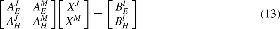
According to equation (13), the electric current and magnetic flux at the structural surface integration points can be obtained. Subsequently, the scattered electric field can be determined using the near-field radiating.^66,67 Finally, the RCS can be calculated using the method mentioned in this section.

Optimization analysis for electromagnetic scattering based on deep learning

Deep learning

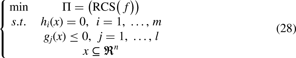
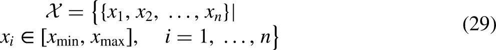
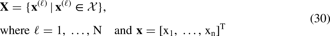
Creating a surrogate model using neural networks is typically done by training on available datasets. This method is significantly faster compared to certain traditional numerical optimization techniques and is particularly effective for addressing nonlinear optimization due to the inherent characteristics of neural networks. In order to minimize the objective function under design variable constraints, an optimization model for problems related to electromagnetic scattering is formulated in the following manner:

$$\{\begin{array}{cc}min& \mathrm{\Pi }=\left(\mathrm{RCS}\left(f\right)\right)\\ s.t.& h_i(x)=0,i=1,\dots ,m\\ & g_j(x)\le 0,j=1,\dots ,l\\ & x\subseteq {\mathrm{\Re }}^n\end{array}$$

(28)

$\mathrm{\Pi }$ represents the objective function; $\mathrm{RCS}(f)$ is a function of frequency $f$ that represents the RCS at a certain angle. $x$ denotes the shape design variables; $h(x)$ and $g(x)$ represent equality and inequality constraints, respectively. The constraints’ numbers are denoted by $m$ and $l$ ; ${\mathrm{\Re }}^n$ denotes the design variables’ domain. The optimization problem in equation (26) under deep learning can be approached through:

• A set of design variables is established for the optimization problem. In this work, the shape design variables are defined by the points that form the shape of the IGA structure. $\mathcal{X}$ represents all design variables and is defined as follows:

  $$\begin{array}{cc}& \mathcal{X}=\{\left\{x_1,x_2,\dots ,x_n\right\}|\\ & x_i\in [x_{\text{min}},x_{\text{max}}],i=1,\dots ,n\}\end{array}$$

  (29)
  The $i$ th design variable is $x_i$ , with its lower and upper bounds being $x_{min}$ and $x_{max}$ , respectively, where $n$ represents the dimensionality of the design variables.

• The initial sample data is obtained through Latin Hypercube Sampling and used as input parameters. The set of $N$ points spanning the entire range of $\mathcal{X}$ generates samples as follows:

  $$\begin{array}{rl}& \mathbf{X}=\{{\mathbf{x}}^{(\ell )}|{\mathbf{x}}^{(\ell )}\in \mathcal{X}\},\\ & \text{where}\ell =1,\dots ,N\text{and}\mathbf{x}=[x_1,\dots ,x_n{]}^T\end{array}$$

  (30)

• Utilizing appropriate numerical methods to assess the solutions in each test case. At each point, $\mathbf{x}$ , the output $y$ of the objective function RCS in this study is evaluated using IGABEM as follows:

  $$\mathbf{Y}=\{\mathrm{RCS}\left({\mathbf{x}}^{(\ell )}\right)|{\mathbf{x}}^{(\ell )}\in \mathcal{X}\},\ell =1,\dots ,N$$

  (31)
  Therefore, the corresponding dataset is generated as $\{({\mathbf{x}}^{(1)},{\mathbf{Y}}^{(1)}),\dots$ , $({\mathbf{x}}^{(\ell )},{\mathbf{Y}}^{(\ell )}),$ $\cdots ({\mathbf{x}}^{(N)},{\mathbf{Y}}^{(N)})\}$ .

• By constructing a neural network for training, the optimization results are obtained. The initial dataset with $N$ samples (where $N=5000$ in this study) is expanded to a larger dataset with $\hat{N}$ samples (where $\hat{N}=\mathrm{50,000}$ in this study) as follows:

  $$\begin{array}{cc}& \{({\mathbf{x}}^{(1)},{\mathbf{Y}}^{(1)}),\dots ,({\mathbf{x}}^{(\ell )},{\mathbf{Y}}^{(\ell )}),\dots ,\\ & ({\mathbf{x}}^{(N)},{\mathbf{Y}}^{(N)})\}\to \{({\mathbf{x}}^{(1)},{\mathbf{Y}}^{(1)}),\dots ,\\ & ({\mathbf{x}}^{(\ell )},{\mathbf{Y}}^{(\ell )}),\dots ,({\mathbf{x}}^{(\hat{N})},{\mathbf{Y}}^{(\hat{N})})\}\end{array}$$

  (32)
  In the extended dataset of $\hat{N}$ (where $\hat{N}>N$ ), the minimum value of $\mathbf{Y}$ determines the optimization result.

Due to the effectiveness of neural networks in training and predicting, as well as their dependence on sample data, two main issues need to be addressed in developing surrogate models for neural network analysis in optimization problems: how to ensure the accuracy of the neural network model and how to ensure the accuracy and sufficiency of the initial sample data. These problems will be discussed later.

GWO algorithm

This section primarily explains how to use the GWO algorithm to enhance the neural network’s capacity for learning and prediction. The purpose of training a neural network is to adjust the weights and biases to find a set of suitable parameters that minimize the loss function. In this study, the accuracy of the model is measured using mean square error loss, with the goal of finding a set of weights and biases that minimize the mean square error loss. During the training of neural networks, local optimization issues often arise, which can affect the model’s generalization performance and prevent it from finding the global optimal solution. The GWO algorithm, as a global search algorithm, can alleviate this issue. The algorithm has the characteristics of few adjustable parameters and easy implementation. It can achieve a balance between local optimization and global optimization, thereby obtaining high-precision solutions while ensuring good convergence speed. Compared to other optimization algorithms, the GWO algorithm is faster because it first produces answers, compares, and ranks them accordingly, and then outputs the best solution. This is similar to the training process of neural networks. This section combines the GWO algorithm with neural networks to enhance the model’s generalization performance. The specific optimization process is shown in Figure 2.

Figure 2.

Gray wolf optimizer-based back-propagation neural network (GWO-ANN) optimization flowchart.

GWO is a novel population-based algorithm inspired by the social behaviors of gray wolves, including their hierarchy and hunting mechanisms. ⁶⁸ The main flow of the GWO algorithm includes three key stages: following, surrounding, and attacking. In GWO, there are four types of wolves belonging to different social classes. The $\alpha$ , $\beta$ , and $\delta$ wolves represent the top three classes and are crucial in determining the primary search directions, while numerous $\omega$ wolves form the lowest class and are responsible for attacking the prey.

GWO represents the optimized parameters using the position vector of each wolf in the wolf pack, with the best parameter values serving as the prey’s position. It simulates the process of wolves encircling and hunting their prey, ultimately achieving parameter optimization. In this context, $\alpha$ represents the optimal solution, $\beta$ and $\delta$ represent the second and third best solutions, respectively, while $\omega$ denotes a candidate solution. The following mathematical calculations are involved during the process of wolves encircling their prey:

$$\{\begin{array}{c}\mathbf{D}=|\mathbf{C}\cdot {\mathbf{X}}_p(t)-\mathbf{X}(t)|\\ \mathbf{X}(t+1)={\mathbf{X}}_p(t)-\mathbf{A}\cdot \mathbf{D}\\ \mathbf{A}=2\mathbf{a}\cdot {\mathbf{r}}_1-\mathbf{a}\\ \mathbf{C}=2{\mathbf{r}}_2\end{array}$$

(33)

where $\mathbf{D}$ represents the distance vector between the gray wolf and the prey; $X_p(\cdot )$ denotes the position vector of the prey; $X(\cdot )$ denotes the individual position vector of the gray wolf; $t$ is the current iteration number; $\mathbf{A}$ and $\mathbf{C}$ are the group synergy coefficient vectors; ${\mathbf{r}}_1$ and ${\mathbf{r}}_2$ are random vectors with elements between [0,1]; and the elements in vector $\mathbf{a}$ linearly decrease from two to zero during the iterations.

Considering that the location of the optimum (prey) is unknown, we preserve the top three best solutions ( $\alpha$ , $\beta$ , and $\delta$ ) from the current state. The other search agents ( $\omega$ ) then update their positions based on the positions of these best search agents, as expressed by:

$$\begin{array}{cc}{\mathbf{D}}_{\alpha }& =|{\mathbf{C}}_1\cdot {\mathbf{X}}_{\alpha }(t)-\mathbf{X}(t)|\\ {\mathbf{D}}_{\beta }& =|{\mathbf{C}}_2\cdot {\mathbf{X}}_{\beta }(t)-\mathbf{X}(t)|\\ {\mathbf{D}}_{\delta }& =|{\mathbf{C}}_3\cdot {\mathbf{X}}_{\delta }(t)-\mathbf{X}(t)|\end{array}$$

(34)

where ${\mathbf{D}}_{\alpha }$ , ${\mathbf{D}}_{\beta }$ , and ${\mathbf{D}}_{\delta }$ represent the distance vectors between $\alpha$ , $\beta$ , $\delta$ , and wolves, respectively. Consequently, the three wolves’ position vectors can be expressed as:

$$\begin{array}{cc}{\mathbf{X}}_1(t+1)& ={\mathbf{X}}_{\alpha }(t)-{\mathbf{A}}_1{D}_{\alpha }\\ {\mathbf{X}}_2(t+1)& ={\mathbf{X}}_{\beta }(t)-{\mathbf{A}}_2{D}_{\beta }\\ {\mathbf{X}}_3(t+1)& ={\mathbf{X}}_{\delta }(t)-{\mathbf{A}}_3{D}_{\delta }\end{array}$$

(35)

where ${\mathbf{X}}_1$ , ${\mathbf{X}}_2$ , and ${\mathbf{X}}_3$ represent the position vectors of $\alpha$ , $\beta$ , and $\delta$ , respectively. The update of the position vector of other wolves represented by ( $\omega$ ) can be written as:

$$\mathbf{X}(t+1)=\frac{1}{3}[{\mathbf{X}}_1(t+1)+{\mathbf{X}}_2(t+1)+{\mathbf{X}}_3(t+1)]$$

(36)

Figure 3 demonstrates how the search agents update their positions in a two-dimensional space based on $\alpha$ , $\beta$ , and $\delta$ . It can be observed that the final position will lie at any point within the circle, determined by the positions of $\alpha$ , $\beta$ , and $\delta$ in the search space. The distances between the individual wolves and $\alpha$ , $\beta$ , and $\delta$ are represented by $D_{\alpha }$ , $D_{\beta }$ , and $D_{\delta }$ , respectively, and the calculation formula is as follows.

Figure 3.

Position updating in gray wolf optimization (GWO).

The GWO algorithm uses the random vector $\mathbf{A}$ to achieve a global search for prey while simulating a decentralized search for prey and gathering prey. The element of the vector $\mathbf{C}$ in the GWO algorithm is randomly selected between $[0,2]$ , and it can randomly strengthen or weaken the impact of prey position. This method is especially useful in the later iteration process, as it allows the optimization to jump out of the region when encountering the local optimum. As a result, in the GWO algorithm, we use the structural parameters (weight deviation) of the neural network as the position vector of the wolves and the minimum of the loss function as the prey for the initial training of the neural network.

In addition, the structure of a neural network plays a crucial role in determining its learning ability. Typically, during the training process of a neural network, parameters are continuously updated to minimize the loss function value. However, since the initial parameters are generally randomly generated, directly training the network often results in parameters converging to a local minimum. Therefore, pre-training can help reduce the risk of parameters falling into a local optimum.

Pre-training methods involve randomly generating various neural network architectures, each of which undergoes iterative training on a small dataset. The evaluation criteria for model fitting ability typically include the determination coefficient and mean square error function. After training, selecting the neural network structure with the best-fitting performance for further use is essential.

In this paper, GWO-ANN is used to optimize the objective function, where GWO and ANN are combined to form a model aimed at accelerating SO in multi-frequency electromagnetic scattering problems. The specific process is as follows: (a) We first define the objective of the problem, which is to minimize the RCS; (b) NURBS is used to construct the geometry; (c) IGABEM is applied for the numerical calculation of the electromagnetic field; (d) The GWO-ANN model is used to optimize the geometric parameters, where ANN estimates the RCS value and GWO optimizes the shape parameters; (e) The geometric shape and electromagnetic simulation results are iteratively updated until the optimization converges; (f) The optimal solution is output, yielding the optimized geometry and the corresponding RCS value.

Numerical examples—IGABEM for electromagnetic scattering

In electromagnetism, the circle model and the airplane model are both idealized models used to describe the interaction of electromagnetic waves with objects. They are often used to analyze and study the scattering and reflection of electromagnetic waves on different objects. Numerical examples are implemented using Fortran code. The effectiveness and accuracy of IGABEM are validated through two test cases. Additionally, the combination of SO and artificial neural networks (ANNs) is also explored.

In the first example, the DIE circular is considered, whose cross-sections are represented using NURBS curves with multiple control points (as shown in Figures 4 and 5). Figure 6 illustrates the impact of TE or TM polarized plane waves on the object. EFIE is used to compute the RCS of lossless and lossy DIE cylinders at $k=1$ , with a radius of 5  $\text{m}$ and $0⩽{\varphi }^s⩽2\pi$ for both backscattering and forward scattering results. By comparing the results with exact solutions in Figures 7 and 8, it is evident that there is a significant agreement between EFIE results and the exact solutions. Furthermore, upon contrasting Figures 7(a) and 8, it can be observed that while the loss of the target material has a minor impact on the overall trend of RCS, it does exhibit a decreasing trend overall.

Figure 4.

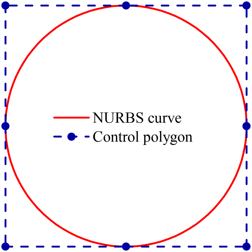
Cylindrical section boundary non-uniform rational B-splines (NURBS) curve and control point.

Figure 5.

Aircraft model diagram. (a) Fighter aircraft model and (b) Non-uniform rational B-splines (NURBS) for fighter aircraft model.

Figure 6.

TE and TM polarized Fields: (a) The TE polarized electric field exists solely in the $z$ -component; (b) The TM polarized electric field contains $x$ and $y$ components. TE: transverse electric; TM: transverse magnetic.

Figure 7.

The RCS for DIE cylinder. (a) The RCS of the DIE cylinder at different angles when $ϵ=5$ and $k=1$ under TE polarized and (b) The RCS of DIE cylinder at different angle when $ϵ$ =5 and $k=1$ under TM polarized. RCS: radar cross-section; DIE: dielectric; TE: transverse electric; TM: transverse magnetic.

Figure 8.

The RCS for lossy DIE cylinder with $ϵ=(5,-108)$ and $k=1$ at different angle under TE polarized. RCS: radar cross-section; DIE: dielectric; TE: transverse electric.

In addition, we also compute the RCS in terms of permittivity. The back-scattering and forward-scattering results are shown in Figure 9. It can be seen that when the permittivity is lower than about 2, RCS increases rapidly with the increase of the permittivity, while when the permittivity is greater than about 2, RCS fluctuates within a certain range. Moreover, RCS is calculated across various frequencies. The backscattering and forward-scattering outcomes are depicted in Figure 10. Despite significant variations in the results, the numerical solution retains high precision and follows a similar trend to Figure 9. It can be seen that although the results change dramatically, the numerical solution can still maintain high precision, while the trend is similar to Figure 9.

Figure 9.

The RCS for DIE cylinder in different terms of $ϵ$ . (a) The RCS for DIE cylinder when $\lambda =5$ and ${\varphi }^s=0$ and (b) The RCS for DIE cylinder when $\lambda =5$ and ${\varphi }^s=180$ . RCS: radar cross-section; DIE: dielectric.

Figure 10.

The RCS of the DIE cylinder at different frequencies. (a) The RCS at different frequency when ${\varphi }^s=0$ and $ϵ=5$ and (b) The RCS at different frequency when ${\varphi }^s=180$ and $ϵ=5$ . RCS: radar cross-section; DIE: dielectric.

To investigate how incident waves affect the distribution of scattering overall, we calculate the scattering field within a $50\times 50$  m area surrounding the cylinder at $\lambda =5$ for various values of $ϵ$ . The real components (unit: V/m) of TE polarized electric and magnetic fields obtained using EFIE are shown in Figure 11. By comparing Figure 11(a) and (b), we observe that the magnitude of the electromagnetic field in lossy media is smaller than that in lossless media. However, there is not a significant difference in the overall distribution of the electric field. This is because in TE polarization, the electric field only exists in the $z$ -direction, whereas in TM polarization, the electric field propagates in both $x$ and $y$ directions. As a result, the current exhibits a similar behavior, ultimately leading to the generation of a more complex scattering field in TM polarization fields.

Figure 11.

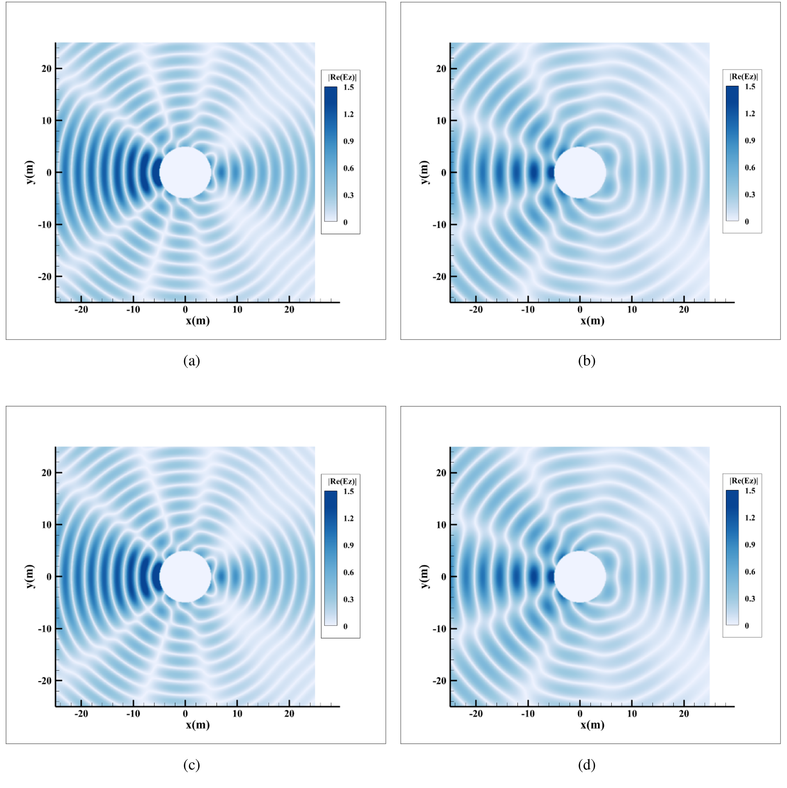
Distribution of the electric field around the dielectric (DIE) cylinder with various $ϵ$ . (a) The field of the DIE cylinder when ${\varphi }^i=0$ for $\lambda =5$ and $ϵ=5$ . (b) The field of the DIE cylinder when ${\varphi }^i=0$ for $\lambda =5$ and $ϵ=(5,-108)$ . (c) The field of the DIE cylinder when ${\varphi }^i=0$ for $\lambda =5$ and $ϵ=8$ and (d) The field of the DIE cylinder when ${\varphi }^i=0$ for $\lambda =5$ and $ϵ$ =10.

Additionally, due to the inherent symmetry of the structure, we observe obvious symmetrical features when analyzing the scattering field. We have also investigated the electric distribution at various incoming frequencies (as shown in Figure 12). It can be observed that, with increasing frequency, the electric distribution becomes more concentrated in the incident direction.

Figure 12.

Distribution of the electric field around the dielectric (DIE) cylinder with various frequencies. (a) The field of the DIE cylinder when ${\varphi }^i=0$ for $\lambda =4$ and $ϵ=5$ and (b) The field of the DIE cylinder when ${\varphi }^i=0$ for $\lambda =2.5$ and $ϵ=5$ .

As is well known, aircraft models play a crucial role in electromagnetics. Studying the electromagnetic scattering characteristics of aircraft models can provide theoretical guidance for the design of stealth fighters. Additionally, using aircraft models can help verify whether algorithms are capable of solving more complex problems. Next, the schematic of this model is shown in Figure 5(a), and the model is constructed using NURBS shown in Figure 5(b). Furthermore, we compute the RCS for DIE fighter aircraft in terms of frequency and $\epsilon$ (see Figure 13). It can be seen that when $\epsilon$ is larger, RCS changes more dramatically with the increase in frequency.

Figure 13.

The RCS for DIE fighter aircraft in terms of frequency and $\epsilon$ . RCS: radar cross-section; DIE: dielectric.

The electric field in terms of frequency is shown in Figure 14. It can be seen that the electric field distribution of the complex model with edges and corners is similar to that of the circular model at lower frequencies, while it becomes more complex at higher frequencies. It can be deduced that at higher frequencies, variations in shape have a more pronounced impact on the scattering field, thereby offering a significant opportunity for effective SO within the operating space.

Figure 14.

Distribution of the electric field around the fighter aircraft.

Numerical examples—SO for electromagnetic scattering

In this section, we discuss the SO for an electromagnetic scattering of the cylindrical model introduced mentioned in Section “Numerical examples—IGABEM for electromagnetic scattering.” The control points of the shape are taken as design variables, and the RCS value is the objective function for optimization. We employ the GWO-ANN method to explore a set of control point coordinates that generate the minimum RCS value, and then use NURBS curves to depict the shape. The training data for the grid is obtained using IGABEM.

SO for an infinite cylinder

We first use the cylinder shown in Section “Numerical examples—IGABEM for electromagnetic scattering” for TE polarization with $\lambda =5$ , $ϵ=5$ . As shown in Figure 5(b), when using NURBS curves, only a few control points are needed to accurately depict the geometric model. To enhance the flexibility of shape adjustments, h-refinement is carried out to augment the degrees of freedom while maintaining geometric precision. In this case, the cylindrical model undergoes refinement scheme one and refinement scheme two, resulting in the number of control points being 13 and 17, as depicted in Figure 15.

Figure 15.

Sectional model boundary. Non-uniform rational B-splines (NURBS) curves and control points with refinement (Example 5.1). (a) Subdivision scheme one and (b) Subdivision scheme two.

As a result of the symmetry exhibited by the model, the control points within the top half of the model are designated as design variables, with their coordinates allowed to vary within a range of 20 $\mathrm{\%}$ . By leveraging Latin-hypercube sampling, responses from 5000 samples across various frequencies are obtained. The approach involves selecting the minimum RCS at ${\varphi }^i={\varphi }^s=0$ as the objective function. Subsequently, the neural network architecture will be trained using these data points as inputs, and the loss function will be the mean square error function.

To further enhance the fitting capability of the neural network, we use the pre-training method mentioned in Section “GWO algorithm.” This network contains five hidden layers with the number of neurons in each layer being: 40, 22, 49, 5, and 30, respectively. The input layer has eight nodes, and the output layer has 1 node, as shown in Figure 16. The neural network optimizer selects the Adam optimizer.

Figure 16.

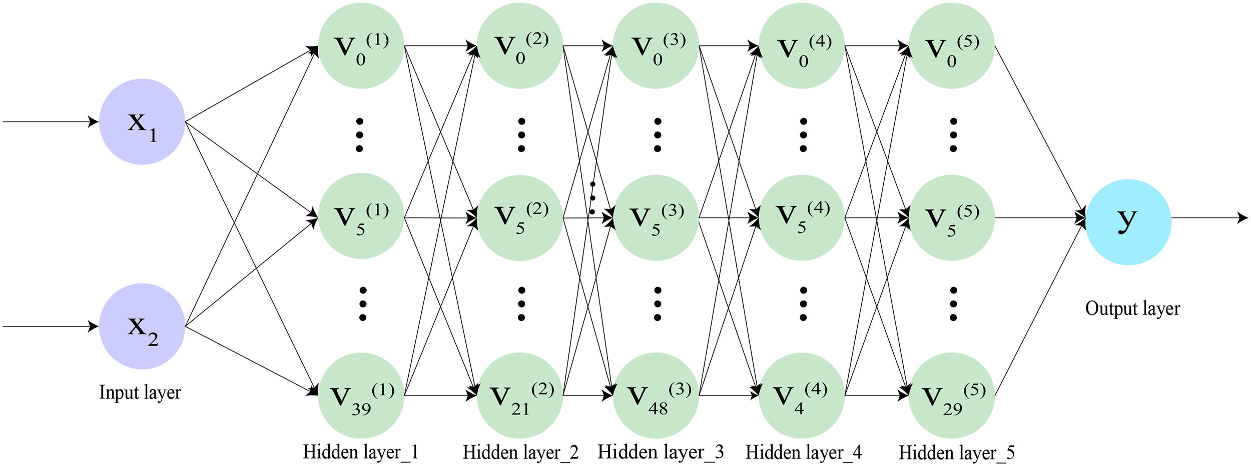
Neural network structure (Example 5.1).

Due to the central symmetry of the model, combined with the fact that the scattering field exhibits axial symmetry along the $x$ -axis when the incident wave is at the 0-degree or 180-degree direction, we designate the top half control points of the model as variables. The design variable selection of subdivision scheme one can be seen in Figure 17 with a similar scheme for subdivision scheme two but fixing the horizontal coordinates of the control points. Furthermore, we use mapping operations to ensure that the upper and lower halves of the model are symmetric. The modified model is shown in the following figures.

Figure 17.

Selection of design variables (Example 5.1).

The results of the optimization and the shape profile are displayed in Figure 18. It is notable that significant improvements have already been observed in the optimization results after 500 iterations of the neural network, reducing the average RCS value from 13.74 to $-$ 4.52. Following 1000 iterations, this improvement further intensified, with the average RCS reaching $-$ 8.85. With subsequent iterations up to 10,000, the average RCS stabilized at $-$ 23.45. Upon analyzing the optimization process shown in Figure 18, it is evident that as the average RCS decreases, the shape progressively shifts toward a sharper profile while closely approximating the actual deformed state. This outcome underscores the advantages of employing NURBS IGABEM for achieving smoother and more precise shape modifications. The use of a minimal number of control points facilitates seamless and natural adjustments across a wide spectrum, underscoring the remarkable effectiveness of this method. Such capabilities are pivotal for efficient SO.

Figure 18.

RCS with the corresponding shape profile in terms of iterations: $\lambda =5$ , TE polarization (Example 5.1). RCS: radar cross-section; TE: transverse electric.

Furthermore, the optimized design models for two design variable selection schemes and the electromagnetic field distributions generated by the models are given in Figure 19. As can be observed, the electric intensity of the optimization zone in Figure 11 is much lower than that of the original model’s electric distribution.

Figure 19.

The final optimization design and electric field performance of the two schemes, radar cross-section (RCS) $=-29.23$ for (B) and $\mathrm{RCS}=-23.45$ for (D) (Example 5.1). (A) Optimization design with one subdivision. (B) Distribution of the electric field of the optimization design with one subdivision. (C) Optimization design with two sudivisions. (D) Distribution of the electric field of the optimization design with two subdivisions.

Conclusion

This work focuses on SO for DIE electromagnetic scattering issues using BEM. BEM primarily involves discretizing the surfaces of structures to address scattering problems in unbounded domains. Furthermore, BEM discretizes only the boundary, without the need to generate a mesh for the entire domain, which helps avoid the complex mesh generation process. Thus, geometric errors are reduced. GWO-ANN is employed to conduct SO in the problems of multi-frequency and wide-angle electromagnetic scattering. Based on comparisons with analytical solutions and computational results of several complex models, we have drawn the following conclusions:

For DIE targets in electromagnetic scattering problems, the calculation results based on IGABEM show high precision.

The employment of GWO leads to superior optimization outcomes in comparison to the conventional ANN approach.

Both types of models’ final optimization results show that NURBS-based modeling not only reduces the dimensionality of design variables, but also makes the shape smoother and more flexible. This method can provide more reasonable data samples for optimization analysis. The results demonstrate that this method is highly effective for RCS optimization design.