Sage Journals: Discover world-class research

Abstract

In this study, we introduce a method for estimating the position of a self-driving solar panel-cleaning mobile robot. This estimation relies on line counts, typically 16 cm in panel width, obtained through image processing on the panel floor, along with wheel encoder information and inertial sensor data. To achieve accurate line counts, we introduce two adjusted threshold values and allow offsets in these values based on the robot's speed. Additionally, inertial measurement unit (IMU) signals assist in determining whether a line is horizontal or vertical, depending on the robot's movement direction on the panel, utilizing the robot's heading angle and detected line angle. When the robot is positioned between lines on the panel, more precise location estimation is necessary beyond simple line counts. To tackle this challenge, we integrate the extended Kalman filter with IMU data and encoder information, significantly enhancing position estimation. This integration achieves an RMSE accuracy value of up to 0.089 m, notably at a relatively high speed of 100 mm/s. This margin of error is almost half that of the vision-based line-counting method.

Keywords

Vision processing sensor fusion extended Kalman filter localization solar panel-cleaning robot

Introduction

According to the International Energy Agency (IEA) energy statistics, the renewable energy sector has experienced significant growth since the 2000s, notably led by solar power within the renewable energy market.¹ This expansion in solar power generation has consequently increased the need for maintenance and repair of solar panels, directly impacting their efficiency in power generation. To address this, solar panel-cleaning robots have been developed to handle tasks that traditionally relied on human labor. Accurate recognition of the robot's location is crucial for effectively managing its autonomous operations in cleaning solar panels.²

Currently, solar panel cleaning robots can be broadly categorized into two types based on their operational methods. The more common type is the manual operation cleaning robots.^3,4 These robots necessitate users to visually inspect and regulate the cleaning range and the robot's driving speed during the cleaning process. Consequently, these robots possess simple mechanisms and do not require additional devices. However, they rely on constant user supervision, and the thoroughness of cleaning relies on the user's expertise. Additionally, the operational stability of the robot, such as the risk of it falling, is determined by the user's skill.

The second type is autonomous cleaning robots. These robots maneuver on the panels independently and conduct cleaning operations without requiring constant user intervention post-initial setup. Equipped with multiple sensors, they follow predetermined paths to clean the panels. Automatic drive cleaning robots come in two variations. One involves robots that continuously clean and traverse the entire panel after installing rails above and below the panels.^5–8 The other variation comprises mobile robots that autonomously navigate along predefined paths to clean the panels.^9–11

Rail-based robots offer the advantage of swiftly cleaning entire panels but come with the drawback of moving at a fixed speed, potentially leading to insufficient cleaning in heavily soiled areas. Conversely, mobile autonomous robots adhere to predetermined rules, traversing the panel surface while calculating displacement to estimate their position and generating navigation paths to avoid re-cleaning areas. However, on sloped panels, accurate displacement calculation and precise movement path determination become challenging, hindering the creation of optimal cleaning paths.

This challenge prompted the development of algorithms for robot localization. Functions to estimate position, implemented using camera images, wheel encoders, and inertia sensors, are integrated into localization algorithms. Previous studies have employed wheel encoders for position estimation, merging inertia sensors or image data to determine the current position.^12–18 Research also explores indoor localization using Wi-Fi,^19–22 ultra-wideband (UWB) communication modules,^23–27 global positioning system (GPS),^28–30 and real-time kinematic (RTK) GPS.³¹^,32

The limitations of conventional GPS, with errors within several meters, and RTK GPS, which introduces error variance based on distance from the reference station, pose challenges for precise robot localization, particularly on inclined solar panels. High-performance RTK GPS units, promising less than 10 cm error, are bulky, heavy, and often expensive, making them impractical for mobile robots maneuvering on inclined panels. Other positioning methods, excluding RTK GPS, exhibit errors in the order of meters, a significant concern given the size of solar panels.

Inaccurate position estimation during path planning for cleaning can lead to duplicated cleaning or missed areas on the panel. The tilted installation of panels aimed at enhancing solar power efficiency further complicates matters, potentially causing slippage for the robot, which in turn introduces errors in position estimation. Existing sensor fusion methods relying on wheel encoders struggle to offer precise measurements, leading to substantial errors in generated cleaning paths. To address these challenges and ensure comprehensive and accurate cleaning paths for solar panels, there is a pressing need to develop technology that enables precise position estimation, especially when robots navigate inclined surfaces and encounter slippage.

This study introduces a unique approach by leveraging a standard camera, wheel encoder, and IMU sensor data. The robot identifies perpendicular straight lines in both horizontal and vertical directions, mirroring the common pattern found on solar panels. Using IMU sensor data, the robot distinguishes between vertical and horizontal lines, tracks these lines as it moves, and estimates its position on the panel by counting the lines passed. Fusing the robot's posture angle from the wheel encoder and inertial sensor data through an extended Kalman filter enhances the accuracy of robot localization on solar panels. This research aims to estimate the location of mobile robots on solar panels using integrated data. To accurately detect panel straight lines, a more precise line count was achieved by setting a double threshold value. Addressing the robot's high speed, line counting was refined by adjusting offset values to accommodate the robot's velocity, even when using a relatively low-cost camera.

Determining the robot's heading angle crucially relies on the robot's roll and pitch angles while navigating inclined solar panels. These angles, along with line count data from image processing, are fused into the extended Kalman filter algorithm to precisely estimate the robot's location between each line in both horizontal and vertical directions.

The structure of this work is organized into sections, starting with the second section covering image processing for precise line identification. The third section focuses on determining the robot's heading angle on a tilted panel, followed by the fourth section, which delves into the location recognition algorithm using the extended Kalman filter. Finally, the fifth section encompasses the experimental results obtained from this research.

Image processing

It is crucial to detect the straight lines on the solar panel to estimate the moving robot's location accurately.³³ Typically, solar panels feature white straight lines against a dark background, as illustrated in Figure 1. In this study, emphasis is placed on counting the thicker horizontal and vertical lines while the robot is in motion, while disregarding the thinner lines between them. The focus is on accurately identifying and counting these main lines for position estimation, ensuring their clear identification.

Figure 1.

Orthogonal line pattern of solar panel.

To achieve this, specific image processing techniques tailored for line detection are employed. The general process for detecting straight lines is depicted in Figures 2 and 3 outlining the overall steps involved in this line detection process. This method aims to precisely identify and count the prominent lines critical for estimating the robot's location on the solar panel.

Figure 2.

Camera placement on the robot.

Figure 3.

Image processes for line detection.

Straight-line detection

It seems like you are describing the initial steps in the image preprocessing phase to detect straight lines using the camera-acquired image. Establishing a region of interest (ROI) aids in minimizing processing time and pinpointing a single straight line accurately. Since the color information is not critical for the line detection process, the image is converted to grayscale using Eq. (1), where R, G, and B denote the intensities of the color components, and $i (x, y)$ represents the converted intensity at the pixel location $(x, y$ ). This conversion to grayscale simplifies subsequent line detection processes by focusing solely on intensity variations rather than color information.

i (x, y) = 0.3 R (x, y) + 0.59 G (x, y) + 0.11 B (x, y)

(1)Next, a binary filter is applied to remove noise in the image. Typically, applying a Gaussian filter smooths intensity values in areas where pixel intensity changes insignificantly, effectively removing noise by averaging neighboring pixel values. However, in regions with rapid intensity changes (edges), the Gaussian filter might inadvertently reduce edge values along with the noise.

To combat this, a bi-directional filter, as outlined in Eq. (2), is employed to address noise removal while preserving edge values of the straight line.³⁴ In this equation, $w_{p}$ represents the normalization constant, ensuring that the summation of the mask of the bi-directional filter equals 1. This filter considers both pixel intensity and distance between pixels simultaneously to effectively remove noise while safeguarding edge information of the detected straight line.

$p and q$ are the pixel coordinates, $G_{σ_{s}} and G_{σ_{r}}$ are Gaussian distribution functions whose standard deviations are $σ_{s} and σ_{r},$ respectively. $i_{p}$ is the pixel intensity, and $i_{q}$ is the intensity of the neighboring pixel.

i_{P} = \frac{1}{W_{p}} \sum G_{σ_{s}} (| p - q |) G_{σ_{r}} (| i_{p} - i_{q} |) i_{q}

(2)Absolutely, once the image has been processed and noise reduced, the next step is to separate the straight line from the background. Given that the straight line appears brighter against the darker background, a binarization technique is applied. This method sets pixel values to 0 or 1 based on a threshold value. Let

α

and

β

be a percentage of pixels belonging to each class based on a threshold value.

σ_{1}^{2}

and

σ_{2}^{2}

are variances of each class and the Otsu method was used to find the threshold value that minimizes Eq. (3).³⁵

σ^{2} = α σ_{1}^{2} + β σ_{2}^{2}

(3)Absolutely, it is crucial to eliminate unnecessary data such as foreign objects or damaged parts that might exist within the image data, as these could lead to false detections during the line detection process. The opening morphology transformation is an effective technique to remove noise, such as foreign objects, from the straight-line data. Once the noise has been removed from the image, the next step involves detecting a group of straight-line candidates using the Canny edge algorithm. This algorithm helps identify edges in the noise-reduced image, highlighting potential straight-line segments. The resultant image after this image processing stage is typically represented as shown in Figure 4.

Figure 4.

Processed images (a) grayscale, (b) bilateral filter, (c) binary, (d) opening, (e) canny edge.

Through the camera installed on the underside of the robot body, lines drawn on the panel floor were recognized. Installing the camera on the floor allowed for better clarity in capturing video images as it blocked surrounding light.

From the detected groups of straight-line candidates, the selection process involves choosing two lines perpendicular to each other while excluding other lines that do not meet this perpendicular criterion. This step helps filter out non-perpendicular lines, focusing on identifying the primary lines of interest that are perpendicular to each other—a common pattern found in solar panels.

It sounds like the robot in this study is capable of moving both forward and backward, but the analysis focuses solely on the straight-line images captured when the robot moves in the forward direction. Even when the robot turns, the images of the lines are obtained from the forward-facing perspective. As a result, a reference point is established, as depicted in Figure 5, to track and analyze the straight-line data consistently across the forward movement and turning instances of the robot. This reference point likely aids in maintaining a consistent frame of reference for analyzing and processing the straight-line images obtained during the robot's movements. The track point is set to the horizontal center value of the image and the moving vertical value can be obtained as in Eqs. (4)–(6). Here, w is the width of the ROI in the image, and $ρ and ϑ$ are used to represent the distance and slope of the straight line in the image coordinates $(u, v)$ driven by the Hough transform. Absolutely, by tracing the reference point of the straight line and counting the number of lines as the robot moves, it becomes feasible to estimate the robot's location on the solar panel.

u c o s ϑ + v s i n ϑ = ρ

(4)

v = \frac{ρ - u c o s ϑ}{s i n ϑ}

(5)

tracing poin t_{i} = (\frac{w}{2}, \frac{ρ_{i} - \frac{w}{2} c o s ϑ_{i}}{s i n ϑ_{i}}), i = 1, 2, \dots

(6)where

ρ

is the distance to the detected line, which is perpendicular to the line and it is determined as the number of lines that are counted.

ϑ

is the angle formed by

ρ

from the image origin. For every detected line,

ρ_{i}

and

ϑ_{i}

are easily determined by simple image processing technique. Thus, the vertical tracing point for every detected line can be derived using Eq. (6), and the horizontal tracing point is selected as a constant equal to half of the panel width:

\frac{w}{2}

Figure 5.

Track point of a detected line.

Straight-line count

The process of estimating the robot's current location by counting the main straight lines as the robot moves, as illustrated in Figure 6, provides a means to determine the robot's approximate position. Considering that the typical distance between these main lines on a solar panel is around 16 cm, successful line counting allows for an estimated resolution of the robot's location at intervals of 16 cm. However, achieving precise location estimation between these lines will be discussed in a subsequent section, aiming for higher accuracy in pinpointing the robot's position on the panel.

Figure 6.

Robot location on a solar panel.

While this approach appears straightforward, straight-line counting can present challenges. Sometimes, line detection might fail, resulting in inaccuracies. Additionally, without prior knowledge of the robot's trajectory, it is unclear whether the robot is counting horizontal or vertical lines as it progresses, which could affect the accuracy of position estimation. These uncertainties highlight the need for robust methods to handle line detection variations and to ascertain the direction of line counting for more reliable location estimation.

The concept you are referencing with the comparator and reference voltage resembles a Schmitt trigger, where changes in the input voltage may cause unpredictable output fluctuations near the reference voltage. To address this unpredictability, two threshold values are often used to ensure a stable and desired output in the Schmitt trigger (Figure 7, left). Inspired by this principle, the introduction of two threshold values, acting as reference values, is implemented in the line detection process. These threshold values serve to recognize a detected line reliably and determine it as a count value. By setting specific thresholds, this approach aims to establish clear criteria for identifying and counting straight lines, ensuring a more robust and consistent detection process despite potential noise or fluctuations in the input data.

Figure 7.

Schmitt trigger inverter (left) and counting line with double thresholds (right).

Implementing two different threshold values based on the direction of the robot's movement is a smart strategy. When the robot moves upward in the vertical direction, resulting in an increase in the v-coordinate of the track point, a higher threshold value is used as a reference. This higher threshold aims to mitigate errors caused by potential noise in this particular movement direction. Conversely, during downward movement, a lower threshold is set as another reference to accommodate the movement and prevent counting errors attributed to noise. The result displayed in the right portion of Figure 7 showcases the variation in the line track point's height over time and how the line-counting value gets updated. As the robot moves vertically, the count increments when it surpasses the upper threshold. Notably, even during instances where noise affects the height of each line at 11,400 and 11,800 ms, the count increases by one without errors, demonstrating the accuracy achieved through the utilization of two different threshold values. This approach effectively ensures an accurate line count by adapting threshold values based on the robot's vertical movement direction, minimizing counting errors caused by noise fluctuations.

Absolutely, variations in shutter speed or image resolution can indeed impact the detection of straight lines in specific frames, potentially affecting the functionality of line counting. While adopting an ultra-high-speed camera could potentially mitigate this issue by securing a larger volume of data through numerous frames per second, this solution demands a costly environment. Absolutely, achieving accurate straight-line counting across different robot speeds, especially with a more affordable camera, necessitates precise adjustments to determine the thresholds.

Correction of threshold value according to robot speed

To account for the robot's speed, the threshold value requires adjustment by incorporating an offset value, as depicted on the right side of Figure 7. The correction procedure unfolds as follows: Given the disparity between camera and robot coordinates, Eqs. (7)–(11) are employed to convert the distance the robot traverses during the sampling time into values within the image coordinates ( $u, v$ ).

From the camera Eq. (7), the point in the image coordinates $(u, v)$ can be drived from the robot coordinates $(x_{r o b o t}, y_{r o b o t}, z_{r o b o t})$ using the calibration matrix $H,$ which is driven by multiplying the camera intrinsic matrix $I^{P_{c}}$ and transformation matrix of robot coordinates with respect to camera coordinates $c^{M_{r o b o t}}$ . Here, s is a scale factor. Also, the rotational matrix of the robot coordinates with respect to the camera coordinates, $c^{R_{r o b o t}}$ can be determined as Eq. (8) when we set the robot and image coordinates as shown in Figure 8. In the camera intrinsic matrix, the focal length $f_{c}$ , horizontal and vertical pixel size $D_{x}$ and $D_{y}$ , and image center ( $u_{0}, v_{0})$ are presumed to be given in advance.

s (\begin{matrix} u \\ v \\ 1 \end{matrix}) = H (\begin{matrix} \begin{matrix} x_{r o b o t} \\ y_{r o b o t} \end{matrix} \\ \begin{matrix} z_{r o b o t} \\ 1 \end{matrix} \end{matrix}) = I^{P_{c}} c^{M_{r o b o t}} (\begin{matrix} \begin{matrix} x_{r o b o t} \\ y_{r o b o t} \end{matrix} \\ \begin{matrix} z_{r o b o t} \\ 1 \end{matrix} \end{matrix})

(7)where

c^{R_{r o b o t}} = r o t (z, - 90 \circ) r o t (x, 180 \circ)

(8)

c^{M_{r o b o t}} = (\begin{matrix} 0 & - 1 & 0 & 0 \\ - 1 & 0 & 0 & 0 \\ 0 & 0 & - 1 & 0 \\ 0 & 0 & 0 & 1 \end{matrix})

(9)

I^{P_{c}} = (\begin{matrix} \frac{f_{c}}{D_{x}} & 0 & \begin{matrix} u_{0} & 0 \end{matrix} \\ 0 & \frac{f_{c}}{D_{y}} & \begin{matrix} v_{0} & 0 \end{matrix} \\ 0 & 0 & \begin{matrix} 1 & 0 \end{matrix} \end{matrix})

(10)

Figure 8.

Coordinates of the robot, the camera, image (z-axis each is omitted).

Thus, the change in the $x_{r o b o t}$ direction for the track point $Δ x_{r o b o t}$ is determined by multiplying the $x_{r o b o t}$ directional robot velocity $V_{x}$ with the sampling time of image acquisition $t_{s}$ as

Δ x_{r o b o t} = V_{x} t_{s}

(11)From

Δ x_{r o b o t},

the variation(

Δ v)

in the image frame's v direction is determined from Eq. (7). Now, the offset is determined as

2 n Δ v

considering the moving speed of the robot. Here, n is the number of frames to correct data loss, which is found to be in the range of 3∼4 in the current system.

Afterward, it is also viable to alter the direction by leveraging the speed variance between the left and right caterpillars. Consequently, an offset value for horizontal directional movement will be introduced, akin to the adjustments made for vertical movement.

To summarize, determining the width of the offset in image coordinates accounts for the robot's movement speed and is subsequently added to the threshold values. Figure 9 illustrates the result of conducting a straight-line count while applying a correction value to the thresholds, maintaining accurate counting even at high speeds. The upper portion of Figure 9 showcases the vertical track point of the line over time during low-speed movement (50 mm/s). As time progresses, the line's height (vertical track point) increases, indicating the line's descent within the image coordinates as the robot ascends. At low speeds, the detected height data appear clustered. Contrastingly, the lower part of Figure 9 represents the counting outcome at a higher speed (80 mm/s). Here, due to limitations like the camera frame rate, there is a wider gap between data points compared to the lower-speed scenario. Nonetheless, it is evident that effective line counting occurs by appropriately configuring the offset for the threshold value.

Figure 9.

Line-counting (upper: 50 mm/s, lower: 80 mm/s).

Heading angle determination

The solar panel, as depicted in Figure 10, is installed at an incline to enhance power generation efficiency. In such an inclined setup, the z-axis of the inertial sensor, positioned on the robot, does not align perfectly with gravity. Consequently, ensuring precise heading angle information, crucial for maintaining the robot's straight movement, becomes challenging. Therefore, an approach to precisely estimate the robot's heading angle on the inclined panel is introduced, utilizing both the panel's tilt angle and the IMU sensor data.

Figure 10.

IMU sensor on robot.

Estimation of heading angle

Suppose the solar panel is inclined at an angle of $θ$ , then the heading angle, which is the angle between $x_{r e f}$ axis in the reference coordinates and $x_{r o t o t}$ axis in the robot coordinates is set as $ϕ$ . From this configuration, we see that the rotational matrix $R_{1}$ generated from $α, β, and γ$ values, which are roll, pitch, and yaw angles measured by IMU (Figure 10) and another rotational matrix $R_{2}$ driven by panel tilt angle and robot's heading angle with respect to the reference frame are identical. By defining two rotational matrices, $R_{1} and R_{2}$ , as shown in Eqs. (12)–(13), the combined transformation must satisfy the condition of equality: $R_{1} = R_{2}$ , thus, the robot's heading angle $ϕ$ can be determined using Eqs. (14)–(16). These equations demonstrate its correlation with the roll and pitch angles of the robot's posture (Figure 11).

R_{1} = r o t (z_{r o b o t}, γ) r o t (y_{r o b o t}, β), r o t (x_{r o b o t}, α)

= (\begin{matrix} c o s γ c o s β & - s i n γ c o s α + c o s γ s i n β s i n α & s i n γ s i n α + c o s γ s i n β c o s α \\ s i n γ c o s β & c o s γ c o s α + s i n γ s i n β s i n α & - c o s γ s i n α + s i n γ s i n β c o s α \\ - s i n β & c o s β s i n α & c o s β c o s α \end{matrix})

(12)

R_{2} = r o t (x_{r e f}, θ) r o t (z_{r o b o t}, ϕ) = (\begin{matrix} c o s ϕ & - s i n ϕ & 0 \\ c o s θ s ϕ & c o s ϕ c o s θ & - s i n θ \\ s i n θ s i n ϕ & s i n θ c o s ϕ & c o s θ \end{matrix})

(13)

Figure 11.

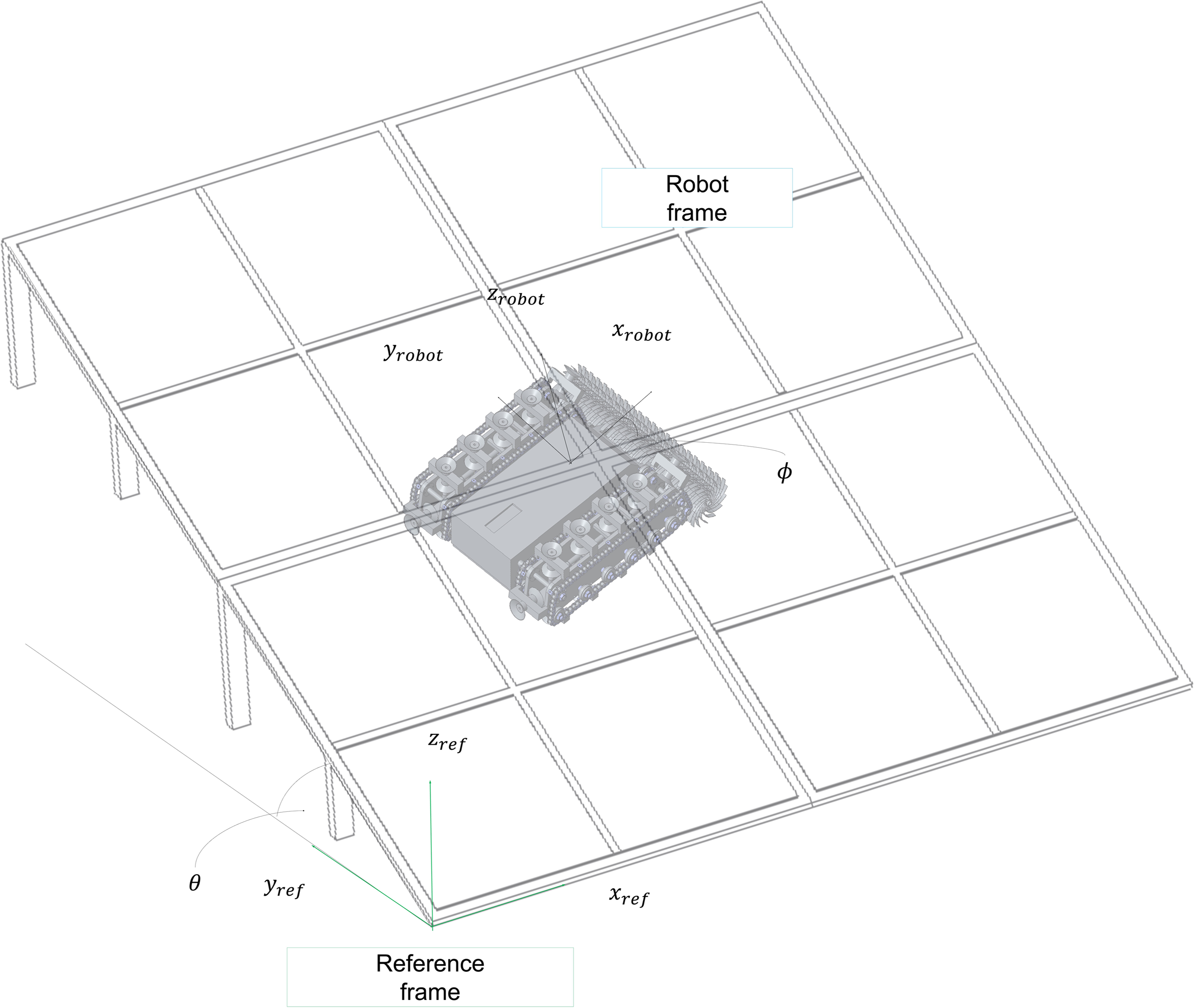
Robot on tilted solar panel.

By selecting (3,1) and (3,2) elements from two rotational matrices $R_{1} and R_{2}$ :

s i n θ s i n ϕ = - s i n β, s i n ϕ = - \frac{s i n β}{s i n θ}

(14)

s i n θ c o s ϕ = c o s β s i n α, c o s ϕ = \frac{c β s i n α}{s i n θ}

(15)the heading angle

ϕ

can be determined as

ϕ = \tan^{- 1} (- \frac{s i n β}{c o s β s i n α})

(16)

Hence, the heading angle of the robot on the inclined surface can be derived from the roll and pitch angles measured by the IMU sensor. This calculated heading angle is utilized for the robot to either move straight on the panel or navigate at a predetermined angle.

Horizontal–vertical discrimination of detected straight lines

The solar panel's horizontal and vertical lines appear visually similar. Despite detecting and counting straight lines through image processing, determining the robot's movement direction—vertical or horizontal—solely from the image remains challenging.

When the robot is in motion, it falls into two defined cases based on the heading angle detailed in the Estimation of heading angle section. For instance, as depicted in Figure 12, if the robot's heading angle $ϕ$ is 0°, it faces the 12 o’clock position of the panel, falling under Case A. Consequently, within the two detected straight lines—one close to 90° and the other at 0°—a line close to 90° indicates a horizontal line, following a similar rule for determining vertical lines.

Figure 12.

Classification of robot's heading angle $ϕ$ and detected line angle $σ$ .

Hence, as depicted in Figure 12, discerning whether the detected straight line represents a horizontal or vertical line depends on the robot's movement direction on the panel. This determination is achieved by integrating the line image data with posture information extracted from the IMU sensor. Implementing this algorithm allowed for two-dimensional location recognition, achieved by incrementing or decrementing count values in response to horizontal and vertical motions during line counting.

Location recognition between lines

In the preceding section, we demonstrated the feasibility of estimating the robot's position by merging the line-counting technique from camera image processing with the heading angle derived from the IMU sensor. However, the line-counting method has a limitation: it does not provide the exact robot position within the line. To address this, we propose a location recognition algorithm that combines image processing using an inertial sensor for line counting and an extended Kalman filter for pinpointing the robot's location between lines. As the robot traverses a line, its new location is updated through line counting, while precise location estimation between lines is achieved via the extended Kalman filter. This section introduces a Kalman filter design tailored for estimating the robot's location as it moves between lines.

Robot model

The solar panel-cleaning robot in this work is a walking-type mobile robot with vacuum adsorption pads on the left and right. It can be modeled as a two-wheel-driven robot as in Figure 13. The kinematics of the robot can be expressed as Eq. (17), where $\dot{x}$ and $\dot{y}$ are the velocities of the robot body center and $\dot{ϕ}$ is the heading angular velocity.

[\begin{matrix} \dot{x} \\ \dot{y} \\ \dot{ϕ} \end{matrix}] = [\begin{matrix} \frac{v_{R} + v_{L}}{2} c o s ϕ \\ \frac{v_{R} + v_{L}}{2} s i n ϕ \\ \frac{v_{R} - v_{L}}{b} \end{matrix}]

(17)where b is the distance between the legs, and

v_{R} = r ω_{R} and v_{L} = r ω_{L}

are linear velocity of the left and right leg, and r is the proportionality factor between linear velocity and motor angular velocity (

ω_{R} and ω_{L})

is measured from the encoder mounted on each leg.

Figure 13.

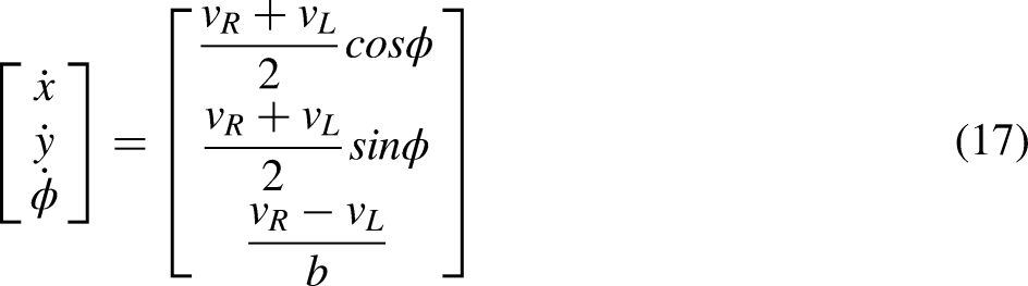
Model of solar panel-cleaning robot.

The robot's location was determined using an IMU (BNO080, manufacturer: Bosch) and encoders (PG42-BL42100B, manufacturer: Motorbank). While the IMU provides posture information through gyroscope and accelerometer data, the yaw angle (heading) is prone to error due to the magnetic field from the robot's driving components. As a remedy, the yaw angle is replaced with the outcome derived in Eq. (16). Estimating the robot's location using encoders within 16 cm-wide lines is susceptible to errors caused by vacuum pad slippage. Hence, this study employs an extended Kalman filter algorithm to fuse encoder and IMU data for estimating the robot's location within lines.^36,37

Extended Kalman filter-based location recognition

The state variables of the robot are set to the position $(x_{k}, y_{k})$ and heading angle $ϕ_{k}$ as shown in Eqs. (18)–(21), and the external control input $U_{k}$ is the angular velocities of the right and left motors ( $ω_{R . k,} ω_{L . k})$ . Also, the output $Z_{k}$ is set to the heading angle that contains the measurement noise.

X_{k} = [\begin{matrix} x_{k} \\ y_{k} \\ ϕ_{k} \end{matrix}], U_{k} = [\begin{matrix} ω_{R . k} \\ ω_{L . k} \end{matrix}]

(18)The model of the robot in discrete time is as follows.

X_{k} = f (X_{k - 1}, U_{k - 1}) + w_{k}

(19)

Z_{k} = H X_{k} + τ_{k}, H = [0 0 1]

(20)

where

f (X_{k - 1}, U_{k - 1}) = [\begin{matrix} \frac{v_{R . k - 1} + v_{L . k - 1}}{2} Δ T c o s ϕ_{k - 1} \\ \frac{v_{R . k - 1} + v_{L . k - 1}}{2} Δ T s i n ϕ_{k - 1} \\ \frac{v_{R . k - 1} - v_{L . k - 1}}{b} Δ T \end{matrix}]

(21)

Here, $v_{R . k - 1}$ and $v_{L . k - 1}$ are right and left velocities of the robot at $k - 1$ step, $w_{k}$ is Gaussian noise with covariance $Q_{k}$ and zero with the average value, which is an error due to the external environment. $τ_{k}$ is the measurement error with the Gaussian noise of covariance $R_{k}$ and zero mean value. $Δ T$ is the sampling time. The predicted position of the robot is as shown in Eq. (22).

{\hat{X}}_{k}^{-} = f ({\hat{X}}_{k - 1}, U_{k - 1})

(22)The robot used in this study is a nonlinear model, thus linearization is needed to estimate the location of the robot to adopt the extended Kalman filter. By linearizing Eq. (21) to the first term by Taylor expansion, it can be expressed as Eq. (23).³⁴ At this time,

A_{k}

is the Jacobian of the robot model for the state of the robot and is expressed as Eq. (24).

X_{k} = A_{k} (X_{k - 1} - {\hat{X}}_{k - 1}) + w_{k}

(23)

A_{k} = {\frac{\partial f}{\partial X} |}_{X_{k - 1}} = [\begin{matrix} 1 & 0 & - \frac{v_{R . k - 1} + v_{L . k - 1}}{2} Δ T s i n ϕ_{k - 1} \\ 0 & 1 & \frac{v_{R . k - 1} + v_{L . k - 1}}{2} Δ T c o s ϕ_{k - 1} \\ 0 & 0 & 1 \end{matrix}]

(24)From the difference between the true position and the estimated position, the estimation error and the covariance matrix were obtained as shown in Eqs. (25)–(26).

{\tilde{X}}_{k} = X_{k} - {\hat{X}}_{k} = A_{k} (X_{k} - {\hat{X}}_{k}) + w_{k} =

A_{k} {\tilde{X}}_{k - 1} + w_{k}

(25)

P_{k}^{-} = E [{\tilde{X}}_{k} {\tilde{X}}_{k}^{T}] = A_{k} \cdot E [{\tilde{X}}_{k - 1} {\tilde{X}}_{k - 1}^{T}] A_{k}^{T} + E [w_{k} w_{k}^{T}] + A_{k}^{T} \cdot E [{\tilde{X}}_{k - 1} w_{k}] + E [w_{k} {\tilde{X}}_{k - 1}^{T}] A_{k}^{T}

= A_{k} E [{\tilde{X}}_{k - 1} {\tilde{X}}_{k - 1}^{T}] A_{k}^{T} + E [w_{k} w_{k}^{T}]

(26)

$E [w_{k} w_{k}^{T}],$ the last term in Eq. (26), is the noise due to the external environment and it is expressed by the covariance matrix S of the control input.

S_{k} = [\begin{matrix} σ_{ω_{R}}^{2} & 0 \\ 0 & σ_{ω_{L}}^{2} \end{matrix}]

(27)

where $σ_{ω_{R}} and σ_{ω_{L}}$ are the standard deviations according to the angular velocity of the left and right motors, respectively.

Next, $B_{k}$ , the Jacobian of the robot model for the control input is expressed as Eq. (28). Normally, the position uncertainty of the robot is added to the uncertainty of the previous state and the uncertain angular velocity of the left and right legs.³¹ Based on this fact, the covariance $Q_{k}$ for the system noise is determined as in Eq. (29). Therefore, a priori covariance $P_{k}^{-}$ is determined by Eq. (30).

B_{k} = {\frac{\partial f}{\partial U} |}_{U_{k}} = [\begin{matrix} \frac{1}{2} Δ T c o s ϕ_{k} & \frac{1}{2} Δ T c o s ϕ_{k} \\ \frac{1}{2} Δ T s i n ϕ_{k} & \frac{1}{2} Δ T s i n ϕ_{k} \\ \frac{1}{b} Δ T & - \frac{1}{b} Δ T \end{matrix}]

(28)

Q_{k} = B_{k} \cdot S_{k} \cdot B_{k}^{T}

(29)

P_{k}^{-} = A_{k} P_{k - 1} A_{k}^{T} + Q_{k}

(30)The output refers to the heading angle computed in the Estimation of heading angle section based on the IMU-measured roll and pitch angles. Consequently, the Kalman gain, state estimate, and error covariance are updated as follows:

K_{k} = P_{k}^{-} H^{T} (H P_{k}^{-} H^{T} + R_{k})^{- 1}

(31)

{\hat{X}}_{k} = {\hat{X}}_{k}^{-} + K_{k} (Z_{k} - H {\hat{X}}_{k}^{-})

(32)

P_{k} = P_{k}^{-} - K_{k} H P_{k}^{-}

(33)where

R_{k}

is the covariance matrix for the measurement noise

τ_{k} .

To summarize, the robot's position and heading angle between lines are estimated by integrating motor encoders and IMU data using an extended Kalman filter algorithm. The comprehensive location estimation process is illustrated in Figure 14. Consequently, the extended Kalman filter enables estimation of the robot's position between panel lines. Consequently, upon the robot detecting a new line via image processing, its location is updated based on the current count of horizontal and vertical lines. This updated location is then augmented by the estimated position of the robot between the current lines using the extended Kalman filter.

Figure 14.

Block diagram of extended Kalman filter-based localization.

The final position ( $x_{k}, y_{k})$ of the robot between $j$ and $j + 1$ line updated by combining the line-counting and EKF as

{(\begin{matrix} x_{k} \\ y_{k} \end{matrix})}_{(j, j + 1)} = {(\begin{matrix} n_{k} \\ m_{k} \end{matrix})}_{j} + (\begin{matrix} {\hat{x}}_{k} \\ {\overset{`}{y}}_{k} \end{matrix})

(34)where

n_{k}

and

m_{k}

are the counting values for the horizontal and vertical direction, respectively, and

({\hat{x}}_{k}, {\overset{`}{y}}_{k})

is the estimated location by EKF.

Experimental results

The algorithm designed to estimate the solar panel-cleaning robot's location, as proposed in this study, was implemented on the robot outlined in Table 1, developed by our team. This robot is a link-driven walking model equipped with vacuum suction pads on both legs, enabling movement on inclined surfaces via individual BLDC motor control (shown as the left in Figure 15). The developed robot is depicted on the right in Figure 15. Key specifications of this robot are provided in Table 1.

Figure 15.

Link mechanism of the walking type robot (left) and manufactured robot (right).

Table 1.

Specifications solar panel-cleaning robot for experiments.

Dimension (W × L × H)	836 × 740 × 277 (mm)
Weight	27 kg
Maximum velocity	160 mm/s (ascending at 30)
Sensor	PG42-BL42100B with encoder, 61:1BNO080
Camera	oCam-1CGN-U640(H) × 480(V)@ 180 fpsGlobal shutter

Figure 15 illustrates two interconnected solar panels with approximately a 3 cm gap and a 30° inclination angle between them. An aluminum frame encases all edges, demanding the robot to traverse this gap between panels without losing vacuum on the pads. The specific panel utilized is the Q.PEAK BFR-G4.4 310 (Hanhwa Q CELLS). The robot's designated moving path is depicted in Figure 16, with the lower-left corner of the panel designated as the starting location at (0,0). Upon completing its designated path, the robot returns to this initial location.

Figure 16.

Localization test on the tilted panel.

The robot's trajectory follows a specific sequence: it ascends a vertical slope initially, then undergoes a clockwise rotation to proceed horizontally. Following this, it makes a 90° clockwise rotation to descend and ultimately returns to its initial starting point. This precise movement path was determined by tracking the robot's position across several image frames, constituting the intended trajectory.

To validate the algorithm's efficacy, an experiment was conducted on an actual solar panel. The robot's true position was recorded at 5-s intervals, and the algorithm's performance was evaluated based on calculated errors at these intervals. This experimental procedure was repeated 10 times, with the robot autonomously following a predetermined route during each iteration.

The error according to the current position $e_{k}$ is accumulated and the total error root mean square error (RMSE) value is computed in Eqs. (35)–(36).

e_{k} = \sqrt{{(x_{r e a l . k} - x_{k})}^{2} + {(y_{r e a l . k} - y_{k})}^{2}}, k = 1, 2 \dots

(35)

R M S E = \frac{1}{N} \sum_{k = 1}^{N} e_{k}

(36)

Figures 17 and 18 exhibit experimental outcomes illustrating position recognition during the robot's movement at 60 mm/s. Notably, during the vertical movement phase on the inclined surface, sliding occurs, causing cumulative errors in the wheel encoders. Conversely, substantial slipping occurs during horizontal movement, leading to a skewed robot heading angle. This slippage contributes to continuous accumulation of position error during horizontal movement at this speed.

Figure 17.

Experimental results for each method.

Figure 18.

Position errors for each method.

When relying solely on line image counting for position estimation, the robot's position remains unchanged until a new line is detected and counted. Consequently, a potential error in position estimation of up to 8 cm, equivalent to half the line width, may occur.

Figures 17 and 18 represent the respective positions of the robot according to positioning methods. “Real” denotes the actual position serving as the basis for error measurement, while “vision” represents the position determined through robot camera image processing. “Odometry” indicates the position calculated using robot sensors, and “EKF + vision” signifies a fused position combining the two methods proposed in this work.

We conducted experiments involving position estimation at different speeds while following the same square trajectory. Table 2 summarizes the RMSE values obtained using three distinct position estimation methods. When utilizing the algorithm proposed in this study, which combines line image counting and an extended Kalman filter, the position between lines is estimated based on IMU and encoder data, and any accumulated error between lines is reset upon encountering a new line.

Table 2.

RMSE values for different moving speeds according to the position estimation methods for a square-typed trajectory (unit: m).

Localization method	60 mm/s	100 mm/s	140 mm/s
EKF (Vision + Odometry)	0.031	0.021	0.076
Vision (only line counting)	0.081	0.068	0.084
Odometer (IMU + Encoder)	0.233	0.443	0.114

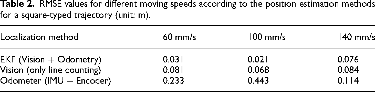
With the incorporation of the EKF algorithm, the average RMSE exhibits a reduction of less than 0.04 m at 60 mm/s and 0.08 m even at higher speeds of 140 mm/s compared to the vision-based method (line-counting).

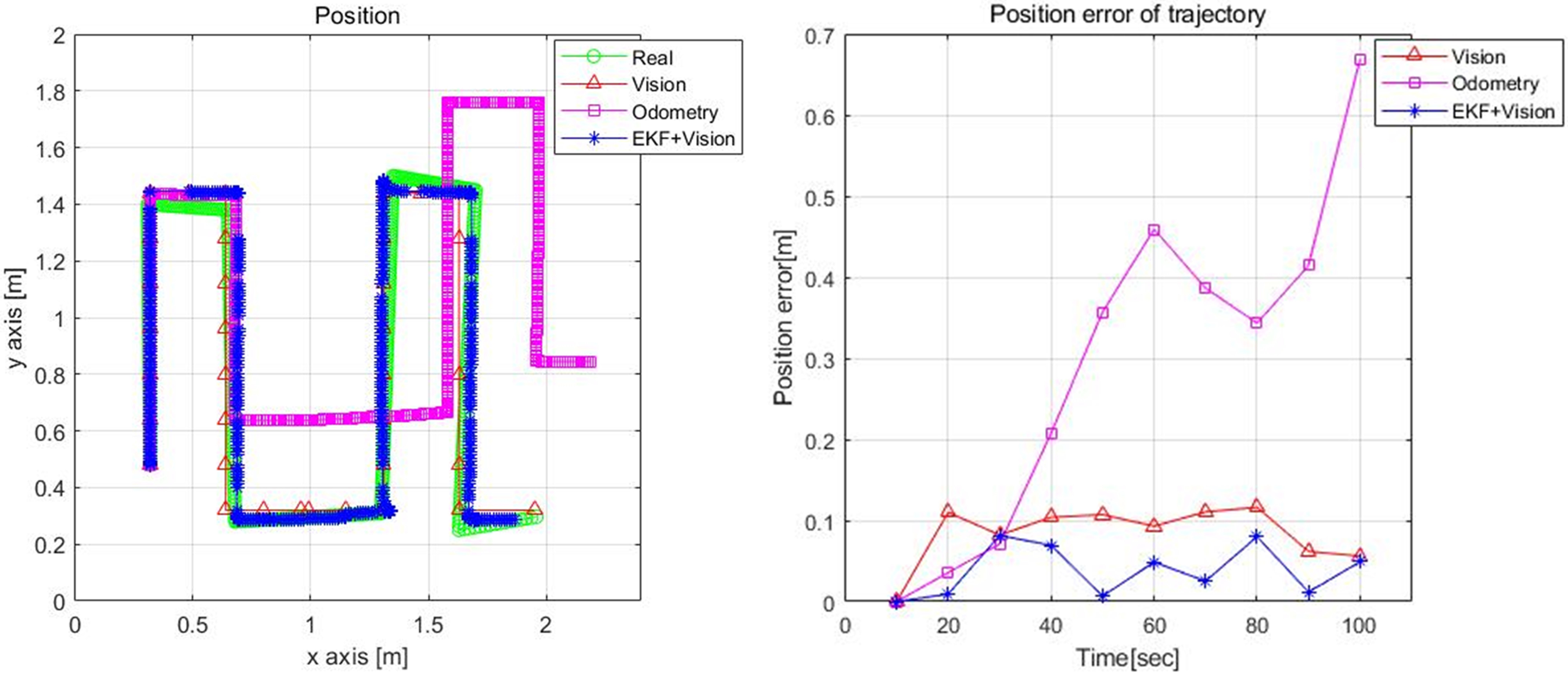
Figure 19 depicts an experiment involving position estimation for a pulse-shaped trajectory, deliberately designed to induce slippage by increasing the number of turns. Figures 20–22 display the results of position estimation under identical speed conditions as the previous experiment.

Figure 19.

Position estimation test setup for another robot moving trajectory.

Figure 20.

Experimental results of position estimation (left) and errors (right) for each method with a moving speed of 60 mm/s.

Figure 21.

Experimental results of position estimation (left) and errors (right) for each method with a moving speed of 100 mm/s.

Figure 22.

Experimental results of position estimation (left) and errors (right) for each method with a moving speed of 140 mm/s.

Table 3 displays RMSE values for position estimation at varying robot speeds during the pulse-shaped trajectory experiment. Similar to previous results, when utilizing the algorithm integrating image line counting and the extended Kalman filter, the average RMSE showcases a decrease of less than 0.02 m and 0.14 m even at high speeds of 140 mm/s compared to the line-counting method.

Table 3.

RMSE values for different moving speeds according to the position estimation methods for a pulse-shaped trajectory (unit: m).

Localization method	60 mm/s	100 mm/s	140 mm/s
EKF (Vision + Odometry)	0.015	0.089	0.134
Vision (line counting only)	0.015	0.169	0.151
Odometer (IMU+ Encoder)	0.360	0.593	0.660

During rapid movements, vacuum release from pads in the walking sequence sometimes leads to inadequate vacuum formation in subsequent steps, causing slippage and substantial cumulative odometry errors. However, employing the extended Kalman filter demonstrates effective position estimation, notably at high speeds of 140 mm/s.

With exclusive reliance on line image counting, estimating position between lines becomes challenging due to continuous slip during robot movement. Increased robot speed exacerbates this slip issue. Combining the EKF method with vision-based line counting yields lower errors compared to simple line counting or odometry-based estimation. This fusion enhances robot position estimation, especially between lines.

Conclusions

This study introduced an algorithm aimed at estimating the position of a solar panel cleaning robot navigating an inclined surface. The algorithm incorporates an extended Kalman filter utilizing data from a wheel encoder and an inertial sensor, along with line-counting through image processing for visible lines on the panel. Notably, the robot's directional movement—whether horizontal or vertical—is determined by interpreting the yaw angle derived from roll and pitch angles obtained from the IMU sensor. This approach is advantageous as it excludes the potentially distorted yaw angle signal, susceptible to influence from the magnetic field surrounding the motor.

This algorithm was designed to estimate the robot's location using only a low-cost camera and IMU sensor, eliminating the need for high-end devices like RTK-GPS or Bluetooth anchors. To enhance accuracy, image processing techniques were employed to eliminate noise on the panel, ensuring the detection of exclusively straight lines. As the robot advances, it actively tracks these detected straight lines and precisely counts them by adjusting upper and lower thresholds according to its speed. This adaptive thresholding minimizes counting errors despite potential image noise.

Furthermore, the algorithm determines whether a detected line is horizontal or vertical by leveraging the combination of roll and pitch angles provided by the IMU. This reliance on IMU data allows for accurate differentiation between horizontal and vertical lines, augmenting the precision of the robot's positional estimation.

To improve the accuracy of robot location estimation between already identified and counted lines, an extended Kalman filter was implemented. This filter utilized the heading angle calculated from the IMU's roll and pitch angles, in conjunction with motor encoder values. Through this estimation method, the robot's position while traversing the inclined panel was reliably determined.

When relying solely on odometry for position estimation, errors between actual and estimated positions tend to increase with the robot's speed and accumulate over longer distances. However, by integrating line-counting via image processing with EKF, utilizing the yaw angle from the IMU and odometry data, the robot's position is initially updated based on line-counting. Simultaneously, more precise estimation of the position between lines occurs, markedly enhancing overall position accuracy regardless of the robot's movement across the panel.

Footnotes

Declaration of conflicting interests

The authors declared no potential conflicts of interest with respect to the research, authorship, and/or publication of this article.

Funding

The authors disclosed receipt of the following financial support for the research, authorship, and/or publication of this article: This research was supported by Korea Evaluation Institute of Industrial Technology grant funded by the Korea Government (MOTIE) (P2004321) and by the Korea Institute for Advancement of Technology (KIAT) grant funded by the Korea Government (MOTIE) (P0008473, HRD Program for Industrial Innovation).

ORCID iDs

Sang Hun Lee

Dong Hwan Kim

Author biographies

Joon Hee Kim graduated from Seoul National University of Science and Technology with a bachelor's degree in mechanical system design engineering in 2018. He graduated from Seoul National University of Science and Technology with master's degree in robotic engineering in 2020. Currently, he has been working at Hyundai Motor Company R&D since 2021.

Sang Hun Lee graduated from Seoul National University of Science and Technology with a bachelor's degree in mechanical system design engineering in 2022. He graduated from Seoul National University of Science and Technology with master's degree in robotics in 2024. Currently, he has been working at Hanwha Precision Machinery Back End Equipment R&D center, Semiconductor Equipment Division since 2024.

Jin Gahk Kim graduated from Seoul National University of Science and Technology with a bachelor's degree in mechanical system design engineering in 2020. He graduated from Seoul National University of Science and Technology with master's degree in robotics in 2022. Currently, he has been working at Hyundai Motor Company since 2022.

Woo Jin Jang graduated from Seoul National University of Science and Technology with a bachelor's degree in mechanical system design engineering in 2019. He graduated from Seoul National University of Science and Technology with master's degree in robotics in 2021. Currently, he has been working at Samsung Electronics' Equipment Technology Research Institute since 2021.

Dong Hwan Kim received his BS and MS degrees from the Department of Mechanical Design and Production Engineering at Seoul National University, in 1986 and 1988, respectively. Also he received a PhD degree from Georgia Institute of Technology, USA. He worked at Korea Institute of Industrial Technology from 1997-1998. He joined Seoul National University of Science and Technology in 1998 as a professor at the Department of Mechanical System Design Engineering. His major research interests are robot control, deep learning, and mechatronics. He is doing numerous projects on robot mechanism and control, artificial intelligence applications to robot, and smart mechatronics system.

References

KEEI. Yearbook of energy statistics. Paris, France: IEA, 2018.

Bae

. Self-location identification and Autonomous moving algorithm for a Solar panel cleaning robot . Master thesis, Seoul National University of Science and Technology, 2017.

Dhanalakshmi

Magesh Raj

Santhosh Kumar

, et al. Solar panel cleaning robot using wireless communication. Annals of RSCB 2021; 25: 17107–17116.

Vishal

Yogesh

, et al. Solar panel cleaning robot. IRJMETS 2022; 4: 485–488.

Ömür

Erdinc

Timur

, et al. A solar panel cleaning robot design and application. EJOSAT 2019; 2019: 343–348.

Shengzan

Lijun

. Research on design of intelligent cleaning robot for solar panel. In: Paper presented at Proceedings of the 20th International Conference on Electronic Business, Hong Kong SAR, China, December 5–8, 2020.

Soniya

Balram

Chandrakant

, et al. Automated solar panel cleaner. IJARIIE 2020; 6: 1–7.

Nagesh

Akshay

Suraj

, et al. Automatic solar panel cleaning system. In: Paper presented at 2nd International Conference on Communication and Information Processing 2020, Talegaon-Dabhade, Pune, India, June 26–27, 2020.

Burak

BÖ

Özge

Gül

. Autonomous solar panel cleaning robot with rubber wheeled and air-absorbing motor. Int J Energy Appl Technol 2020; 19: 182–187.

10.

Nazihah

Mohd

. Development of solar panel cleaning robot for residential sector. EEEE 2023; 4: 606–614.

11.

Sufyan

Thanoon

Hassan

, et al. “UTU” compact solar panel cleaning robot. IJANSER 2023; 7: 217–226.

12.

Kwon

. GPS/INS fusion using multiple compensation method based on Kalman filter. IEIE 2015; 52: 190–196.

13.

Aguiar

Maximo

Yoneyama

, et al. Kalman filtering for differential drive robots tracking. In: Paper presented at XIII Simp´osio Brasileiro de Automa¸c˜ao Inteligente, Porto Alegre RS, Brazil, October 1–4, 2017.

14.

Jetto

Longhi

Venturini

. Development and experimental validation of an adaptive extended Kalman filter for the localization of mobile robots. IEEE Trans Robot Autom 1999; 15: 219–229.

15.

Van Nguyen

Phung

Tran

, et al. Mobile robot localization using fuzzy neural network based extended Kalman filter. In: Paper presented at IEEE International Conference on Control System, Computing and Engineering, Penang, Malaysia, November 23–25, 2012.

16.

Shunya

Toshihiko

Masanori

, et al. Autonomous mobile robot for outdoor slope using 2D LiDAR with uniaxial gimbal mechanism. JRM 2020; 32: 1173–1182.

17.

Byunghee

Gyeongsu

Yesjin

, et al. Loosely coupled LiDAR-visual mapping and navigation of AMR in logistic environments. KROS 2022; 17: 397–406.

18.

Ehsan

. Self-localization for autonomous driving using vector maps and multi-modal odometry . Doctor thesis, University of Waterloo, 2023.

19.

Bobescu

Alexandru

. Mobile indoor positioning using Wi-Fi localization. Review of the Air Force Academy 2015; 1: 119–122.

20.

Biswas

Veloso

. WiFi localization and navigation for autonomous indoor mobile robots. In: Paper presented at 2010 IEEE International Conference on Robotics and Automation, Anchorage, Alaska, May 3–8, 2010.

21.

Lim

Wan

, et al. A real-time indoor WiFi localization system utilizing smart antennas. IEEE Trans Consum Electron 2007; 53: 618–622.

22.

Yang

Shao

. WiFi-based indoor positioning. IEEE Commun Mag 2015; 53: 150–157.

23.

Sczyslo

Schroeder

Galler

, et al. Hybrid localization using UWB and inertial sensors. In: Paper presented at 2008 IEEE International Conference on Ultra-Wideband, Hannover, Germany, September 10–12, 2008.

24.

Zhang

Kuhn

Merkl

, et al. Accurate UWB indoor localization system utilizing time difference of arrival approach. In: Paper presented at IEEE Radio and Wireless Symposium, San Diego, California, USA, October 17–19, 2006.

25.

Krishnan

Sharma

Guoping

, et al. A UWB based Localization System for Indoor Robot Navigation. In: Paper presented at IEEE International Conference on Ultra-Wideband, Singapore, September 24–26, 2007.

26.

Zhou

Law

. Guan YL chin F. Indoor elliptical localization based on asynchronous UWB range measurement. IEEE Trans Instrum Meas 2011; 60: 248–257.

27.

Nguyen

Phan

. Application of SLAM & UWB for self-propelled robots in agricultural production and harvesting. JASAE 2022; 18: 1105–1112.

28.

Kim

Lee

Cheon

, et al.

Design and flight tests of a drone for delivery service.

J Inst Control Robot Syst 2016; 22: 204–209.

29.

Sasiadek

Wang

Zeremba

. Fuzzy adaptive Kalman filtering for INS/GPS data fusion. In: Paper presented at Proceedings of the 2000 IEEE International Symposium on Intelligent Control held jointly with the 8th IEEE Mediterranean Conference on Control and Automation (Cat. No.00CH37147), Rio Patras, Greece, July 19, 2020.

30.

Mohammad

. Positioning accuracy improvement in high-speed GPS receivers using sequential extended Kalman filter. IET Signal Proc 2021; 15: 251–264.

31.

Park

Lee

Jung

. Analysis of position accuracy for underground facility using RTK-GPS. JKSGPC 2003; 21: 237–243.

32.

Elad

. On the origin of the bilateral filter and ways to improve it. IEEE Trans Image Process 2002; 11: 1141–1151.

33.

Liu

. Otsu Method and K-means. In: Paper presented at Ninth international Conference on Hybrid Iintelligent Systems, Shenyang, China, August 12–14, 2009.

34.

Yim

Seok

Lee

. State estimation of the nonlinear suspension system based on nonlinear Kalman filter. In: Paper presented at 12th International Conference on Control Automation and Systems, JeJu Island, Korea, October 17–21, 2012.

35.

Lee

. A new style of sonar sensor array for extended Kalman filter based localization of mobile robots. KSMT 2017; 19: 518–524.

36.

Kim