Sage Journals: Discover world-class research

Abstract

Experimental and numerical analysis of active and passive flow control is an important topic of practical value in the study of turbulent flows. This paper numerically analyzed the effects of an air microjet on an adverse pressure gradient turbulent boundary layer over a flat plane. Experimental data were employed to verify the numerical modeling. Vortex formation and development were then studied by changing the microjet to inflow velocity ratio (VR) and microjet angles. According to the results, the best values of the angles $α$ and $β$ for various velocities were found to be 30° and from 60° to 90°, respectively. Moreover, at VRs = 1, 2, and 4, the $x / L$ values (the distance at which the complete vortex persisted in the flow) were 0.058, 0.078, and 0.18, respectively. Compared to VR = 1, the vortex strength for VRs = 2 and 4 grew by 3.5 and 6.8 times, respectively. When the microjet was added to the flow, the highest variation in the Reynolds stress along the x-direction from VR = 1–4 was 10%. The corresponding values along the y and z- directions were 15% and 2.7 times, respectively.

Keywords

Air microjet turbulent flow vortex formation and dissipation numerical solution

Introduction

An adverse pressure gradient occurs when the static pressure increases in the direction of the flow. So, the boundary layer size and the boundary layer velocity directly above the wall increase and decrease respectively. For a large enough adverse pressure gradient, the boundary layer velocity direction changes and so the boundary layer separates. This local phenomenon is accompanied by the stall (the creation of large vortices, an increase of the drag, and a decrease of the lift). The location of this separation can be delayed by some flow control methods. Flow control methods are divided into passive (no external source of energy is required), and active (an external source of energy is required). The energy is transferred from the main flow to the boundary layer in the passive flow control method. Also, the energy is transferred from some external source of energy to the fluid in the active flow control method.^1–3 One of these active control methods is the vortex generator jet (VGJ) method. This technique is resembles a well-known method of using a small vane vortex generator.⁴ VGJs have some obvious advantages over vane vortex generators, for example, they do not suffer from drag penalties and they can use in the active flow control system. However, experimental or CFD modeling the flow with VGJs is more difficult and costly than that for vane vortex generators.⁵ A pair of counter-rotating vortices (CVPs) are formed by VJGs. The formation mechanism of counter-rotating vortex pairs is not yet fully understood. It is often accepted that the formation of a CVP has roots in the surface of the jet. If the jet is placed closer to the surface, one of the vortices of the CVP is also forced closer to the surface, increasing in losses for this vortex. This reduces the power of the vortex so much as to bring it to the verge of annihilation. The CVP tends to blend into a single vortex as a result of the strength distributed between the two counter-rotating vortices. The weaker vortex is annihilated as it spins around the dominant vortex.^6,7 The secondary vortex structure is also moved toward the outlet if the jet is slanted. As it mentioned, the VGJs can be used in some problems to delay or eliminate flow separation due to the adverse pressure gradient boundary layer. So far, a lot of research was done using CFD or experimental methods to investigate the effect of the VGJs on fluid flow.

McCurdy⁸ was possibly the first researcher to investigate the effects of vortex generators (VGs) on boundary-layer flow control on an airfoil. Wallis⁹ compared an inclined active VG jet (VGJ) and an inclined passive vane VG (VVG). According to his investigation, VGJ arrays would have a very similar impact on a flow as an array of VVGs. Pearcey⁴ was the first researcher that investigated the results of using the VVGs and the VGJs for boundary layer separation control. Rixon and Johari,¹⁰ Ortmanns and Kähler,¹¹ and some other researchers have experimentally investigated Single steady blowing VGJ setups. In this researches, the general VGJ design parameters were the pitch angle, the skew angle, the jet velocity, and the distance between the jets. Rixon and Johari¹⁰ shown that the circulation and the peak vorticity decrease exponentially with growing stream-wise position x. Also, the circulation and peak vorticity and also the average wall-normal position of the primary vortex increase linearly with an increase in the velocity ratio. Ortmanns and Kähler¹¹ investigated the effects of a VGJ on the shear-layer interactions and the turbulent characteristics of the boundary layer. They reported that using a VGJ has a small effect on the turbulent kinetic energy. Also, the mixing is effected large-scale momentum transport. Von Stillfried et al.¹² reported that the actual boundary-layer conditions and many combinations are possible very important in the optimizing parameters of VGJs. According to this investigation, optimum ranges for the pitch angle and skew angle are between 15°–45° and 90°–135°, respectively. Lasagna et al.¹³ investigated Stream-wise vortices originating from synthetic jet–turbulent boundary layer interaction by experimental method. According to these results, the leeward vortex intensified while the other became weaker by increasing the slot yaw angle. Also, the vortices grew in size and intensity by increasing the jet velocity ratio and the slot yaw angle. Feng et al.¹⁴ studied a model of the trajectory of an inclined jet in incompressible crossflow. Also, the effect of jet entrainment, the horseshoe, and wake vortices may create a low-pressure region on the wall and hence alter the jet trajectory and influence the circulation in low-velocity ratios and skew angle near 90°. Beresh et al.¹⁵ investigated the influence of the fluctuating velocity field on the surface pressures in a jet/fin interaction by experimental method. According to this result a counter-rotating vortex pair that passes above the fin is produced by a normal nozzle. Also, pressure fluctuations are principally driven by the jet wake deficit and the wall horseshoe vortex. Also, the inclined nozzle produces a vortex pair. This vortex pair impinges the fin and so yields stronger pressure fluctuations driven more directly by turbulence emanating from the jet mixing. Alimi and Wünsch¹⁶ investigated active flow control of canonical laminar separation bubbles by steady and harmonic vortex generator jets using direct numerical simulations. According to this result disturbances caused by VGJs make the large-scale coherent structures. So the separated region is limited due to the effect of these structures at increasing the momentum exchange. Szwaba et al.¹⁷ investigated the influence of rod vortex generators on a flow pattern downstream using experimental and numerical methods. They put out a rod instead of a jet. They wanted to show that the application of a rod can introduce the same effect as a jet and so introduced a new flow control method dedicated mainly to external flows. Liu et al.¹⁸ used the compression corner calculation model and conducted detailed numerical investigations in the supersonic flow field. They studied the effects of different injection pressure ratios, various actuation positions, and different nozzle types. Also, they mentioned that the distance between the counter-rotating vortex pair and the wall surface is an important factor. As mentioned, with the injection of micro-jets, vortices are formed in the boundary layer through which the momentum is injected from the free stream to the boundary layer and the fluid flow remains near the wall, thus delaying the separation of the flow.

This paper used FLUENT software to analyze the effects of velocity and microjet angles on the turbulent flow over a surface. The strength and stability of the vortices were examined by varying these parameters. The location of the vortex with respect to the boundary layer and its formation and dissipation mechanisms were thoroughly discussed. The velocity and Reynolds stresses on the edges and in the center of the vortex were also explored. Finally, optimized velocity and angles were suggested based on the presented discussions.

Governing equations and numerical modeling

The geometry of the experimental wind tunnel was modeled as shown in Figure 1, where the dimensions, the origin of the coordinate system, and the boundary conditions are specified. The model dimensions in the x and z directions were 3.5 and 0.5 m, respectively. The values of y at the inlet and outlet ends of the tunnel were 0.13 and 0.231 m, respectively. The microjet was located 1.13 m from the inlet of the tunnel. It was 0.001 m in diameter and located 0.005 m from the line z = 0 m at the bottom of the channel. The following figure shows the location of the microjet and its angles from the coordinate axes. 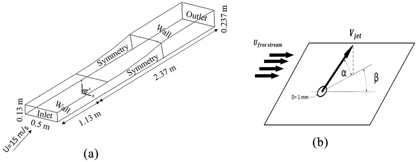The fluid considered was air with viscosity $μ = 1.81 \times 10^{- 5} kg / s m$ and density $ρ = 1.12 kg / m^{3}$ . The inflow velocity was 15 m/s and its turbulence intensity was 2%. The ratio of turbulent to molecular viscosity at the inlet and outlet boundaries was set to 5% and 10%, respectively. Table 1 presents the geometrical definitions of the problem as well as its inputs and outputs.

Figure 1.

Dimensions and boundary conditions of the computational domain: (a) all the domain and (b) near the microjet.

Table 1.

Parameter values.

Parameter	Definition	Parameter	Definition
V _jet = 15, 30,and 60 m/s	Fluid microjetvelocity	L = 3.5 m	Total surface length
$ρ = 1.12 kg / m^{3}$	Fluid density	d = 0.001 m	Microjet diameter
$μ = 1.81 \times 10^{- 5} kg / s m$	Fluid viscosity	h = 0.005 m	Distance of themicroject from thecenter of the surface
U = 15 m/s	Inflow velocity	$α = 30 °, 45 °, 60 °$	Pitch angle of jet hole
IT = 2%	Turbulence intensity	$β = 30 °, 45 °, 60 °, 90 °$	Skew angle of jethole relative to xdirection
$μ_{t} / μ = 5 % - 10 %$	Ratio of turbulent to molecular viscosity	V _jet = 15, 30,and 60 m/s	Fluid microjet velocity

Boundary conditions

Once the computational domain is partitioned into a grid, boundary conditions can be defined on surfaces. The following boundary conditions were used in the modeled wind tunnel shown in Figure 1: Inlet boundary conditions: Inflow velocity or pressure can be defined at the inlet boundaries. An inflow velocity boundary condition is used to determine the velocity and scalar properties of the flow at the inlet boundaries. The flow enters the computational domain at a velocity equal to the values assigned to the nodes on the selected boundary surface.

Wall boundary conditions: All the nodes selected to define this boundary condition move as a rigid body. The no-slip condition is established for such problems, where the wall and its adjacent fluid layer move with the same velocity. Walls in this type of boundary conditions are usually either stationary or moving at a specific speed parallel or perpendicular to the wall surface.

Symmetry boundary conditions: When a simulation is symmetrical from a geometric or flow standpoint, symmetry boundary conditions can be employed. Using this type of boundary, one can cut the number of cells by half, and thereby reduce computational time. In symmetry boundary conditions, there is zero gradients at the boundary along any line perpendicular to it, and no flow passes through the boundary. In other words, at the boundary, normal components of the velocity and gradients of all the variables in a direction normal to the boundary are zero.

Outlet boundary conditions: This type of boundary condition is used in flow simulations where flow properties are not known at the outlet. For all flow regimes simulated using outlet boundary conditions, no flow parameter at the outlet boundaries is specified directly. In fact, such parameters in the simulation are calculated by extrapolating the values from the inside of the computational domain.

Governing equations

Navier-Stokes equations were used to solve the surface flow. However, as the inlet flow was turbulent, their direct modeling requires considerable time and computational costs. Therefore, the governing equations were expanded into RANS equations and solved numerically. The equations were discretized using the finite volume method and velocity and pressure fields were coupled through the SIMPLE algorithm. The momentum and pressure equations were discretized using the second-order upwind scheme. Turbulent flow modeling was carried out using SST-Kω and turbulence was modeled by using the first-order upwind scheme.

So, in order to solve the RANS equations, the continuity and momentum equations in incompressible flow are used as in equations (1) and (2) respectively:¹⁹

div (\vec{v}) = \nabla \cdot \vec{v} = 0.0

(1)

\frac{\partial \vec{V}}{\partial t} + (\vec{\nabla .} \vec{V}) \vec{V} = \frac{1}{ρ} \vec{\nabla} . σ + \vec{g}

(2)

where $σ$ is stress tensor and is equal to:

σ_{ij} = - p δ_{ij} + 2 (μ + μ_{t}) S_{ij}

(3)

where $p, S, μ, V, ρ$ and $δ_{ij}$ are static pressure, strain tensor rate, dynamic viscosity, fluid velocity, fluid density, and Kronecker delta function respectively. Also, μ_t is turbulence viscosity which should be calculated with the SST-Kω model.^20,21

It is worth noting that the parameter $ν_{t} = μ_{t} / ρ$ representing dynamic viscosity was calculated through SST-Kω. In using the SST-Kω model, the transfer equations for turbulence kinetic energy and specific dissipation rate were solved coupled with the equations above. Here, $G_{k}$ is the turbulence kinetic energy generated due to average velocity gradients, and $G_{ω}$ is the generated specific dissipation rate. $Γ_{k}$ and $Γ_{ω}$ denote the diffusion effects of $k$ and $ω$ , respectively, whereas $Y_{k}$ and $Y_{ω}$ represent dissipations of $k$ and $ω$ , respectively. $D_{ω}$ represents cross-diffusion, and $S_{k}$ and $S_{ω}$ are sources defined by the user.^20,21

\frac{\partial (ρ k)}{\partial t} + \frac{\partial (ρ k u_{i})}{\partial x_{i}} = \frac{\partial}{\partial x_{j}} (Γ_{k} \frac{\partial (k)}{\partial x_{j}}) + G_{k} + Y_{k} + S_{k}

(4)

\frac{\partial (ρ ω)}{\partial t} + \frac{\partial (ρ ω u_{i})}{\partial x_{i}} = \frac{\partial}{\partial x_{j}} (Γ_{ω} \frac{\partial (ω)}{\partial x_{j}}) + G_{ω} + Y_{ω} + D_{ω} + S_{ω}

(5)

Resulting from flow velocity fluctuation terms, Reynolds stresses were modeled by considering turbulent viscosity. For incompressible flows, Reynolds stresses were calculated as follows.

- ρ \bar{{u'}_{i} {u'}_{j}} = μ_{t} (\frac{\partial \bar{u_{i}}}{\partial x_{j}} + \frac{\partial \bar{u_{j}}}{\partial x_{i}}) - \frac{2}{3} ρ k δ_{ij}

(6)

Verification of the results

As stated earlier, this paper numerically analyzed the effects of a microjet on a turbulent surface flow. For this purpose, grid-independence tests were carried out by evaluating the numerical results. The results from the numerical model and those from the experimental wind tunnel were also compared and the validity of the numerical modeling was verified.

Figure 2 depicts the present geometry, for which a HEX mesh is used for grid generation. The mesh is finer in regions with more important and intensified flow variations, such as the lower and the inlet boundaries of the domain.

Figure 2.

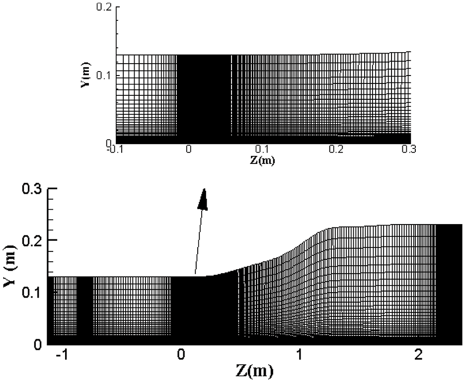
The mesh file used for the computational domain.

To perform the grid-independence test for the case without a microjet, a comparison was made between three mesh densities: coarse, normal, and fine grids having (332 × 45 × 140), (547 × 65 × 140), and (910 × 85 × 140) nodes, respectively. Figure 3 compares the pressure coefficients at the bottom surface of the wind tunnel. It is observed that the pressure decreased almost linearly with a pressure drop in the front portion of the plane. Moving toward the regions with larger distances across the walls, one observes a pressure increase according to Bernoulli’s equation due to lower velocities in the longitudinal direction. A close correlation is also observed among the results from the different mesh densities. Nevertheless, there is a slight difference between the results from the coarse grid and those from the other two mesh densities. The largest difference occurred at x = 1.3 m and was below 1%.

Figure 3.

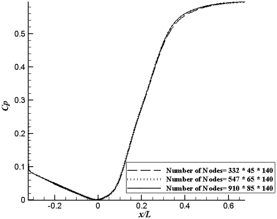
Comparison of Cp for different mesh densities at the lower wall.

Figures 4 present the x and y components of the velocity for a line parallel to the y axis at x/L = 0.1714 m. As the figure shows, the velocity was zero near the wall and gradually increased at points farther from the bottom, up to a distance of about $\frac{y}{δ} = 1$ , after which it remained constant. The y component [of the velocity], however, was constantly growing due to the increasing distance across the walls. A difference is also observed in the results for the coarse grid and those for the other two mesh densities in regions with more intense variations. There was also about less than 1% discrepancy among the results in this case.

Figure 4.

Comparison of velocity for different mesh densities: (a) u and (b) v.

The values for y⁺ over the lower walls of the tunnel are shown in Figures 5. It is observed that the value of y⁺ along the centerline at the lower wall was below the permissible range (about 300²⁰). This confirms the mesh was acceptable near the walls for a turbulent flow.

Figure 5.

Values of y+ at the lower wall of the wind tunnel.

The results for the two turbulence parameters u′u′ and u′v′ at x/L = 0.1714 from the origin along the y-direction are shown in Figure 6 for comparison. The figures show that these parameters grew sharply from zero at the lower boundary, after which they take a zero value in regions closer to the middle of the tunnel, where there was almost no velocity variation. The difference in the results at points near the lower boundary was less than 1%.

Figure 6.

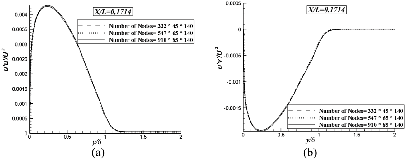
Comparison of the Reynolds stress for various mesh densities: (a) u′u′ and (b) u′v′.

The results indicate that the three mesh densities could provide reasonable accuracy for the present problem. However, adding a microjet resulted in more substantial velocity variations near the boundary and led to larger errors in the case of the coarse grid. Therefore, the normal grid density was chosen for the next stages of the analysis.

The verification experiment was completed in a low speed closed–circuit boundary layer wind tunnel. An adverse pressure gradient turbulent boundary layer with and without the microjet was measured. Hot-wire technique was applied to measure the flow velocities and Reynolds stresses. According to the uncertainty analysis of Anderson and Eaton,²² the mean velocity had an uncertainty of 3% of the local stream-wise velocity. The normal Reynolds stress components had an uncertainty of 5% of the local value of $\bar{u'^{2}}$ . The shear stress had an uncertainty of 10% of the local value of $\bar{u' v'}$ .

To verify the numerical modeling, Figures 7 and 8 present a comparison of the experimental and numerical pressure coefficients and Reynolds stresses on the lower wall of the wind tunnel, good agreement is observed between the experimental and numerical pressure coefficients as shown in Figure 7. A 3% difference is observed between the numerical and experimental results, which is due to the geometric inconsistencies (in the upper curve) of the actual tunnel and the (not completely symmetrical) wall boundary conditions.

Figure 7.

Comparison of the numerical and experimental pressure coefficients.

Figure 8.

Comparison of numerical and experimental Reynolds stresses u′u′ and u′v′: (a) x/L = 0.0171, (b) x/L = 0.1057 m, (c) x/L = 0.2057, and (d) x/L = 0.28 m.

Figures 8 show the numerical and experimental Reynolds stresses at different cross-sections of the turbulent boundary layer. The results indicate that there is good agreement between the numerical and experimental values. However, there is a slight difference in some cases. While many cases showed a difference lower than 2% between the experimental and numerical values, the difference grew to 9% for some other cases. This might be the result of probable experimental errors due to measurement sensitivities. However, the numerical results were concluded to be reasonably accurate.

As mentioned before, the purpose of this paper is to investigate the effects of microjet on the turbulent flow boundary layer with adverse pressure gradient. In fact, by injecting a jet, a longitudinal vortex is formed in the boundary layer. Due to its strength, this vortex forms along and affects the boundary layer until it dissipates. The main idea behind this longitudinal vortex is to form an effective rotational structure resulting from momentum transfer between a cross jet and the main flow. The fluid is injected through a small hole on the surface at a specific angle into the main flow. This creates a vortex moving down flow. Figure 9 shows the longitudinal vortex streamlines due to a microjet with VR = 1, and angles β = 60°, α = 30° at different sections along with the boundary layer. In this figure, the vortex dissipation is well seen in the turbulent boundary layer. The circular motion of the vortex also causes the mass and momentum to be transferred into the boundary layer, making it thinner on one side and thicker on the other. Reynolds stress and velocity components on the surface and consequently the pressure gradient in the boundary layer are affected by the rotational motion of the vortex in the boundary layer of the turbulent flow.

Figure 9.

Velocity contours and vortex dissipation: (a) longitudinal vortex streamlines at different sections and (b) vortex effect on streamwise velocity contours.

Figure 10 compares the experimental and numerical results for a surface flow with a microjet. The comparison was made at 9 cm from the microjet by considering u/U for VRs = 1, 2, and 4 correspondings to percentage errors of 1%, 3%, and 5%, respectively. As the figure shows, there is good agreement between the experimental and numerical results. It was concluded that the numerical results could be used in further stages through the analysis process.

Figure 10.

Comparison of the numerical and experimental results for u/U contours for various microjet velocities at x = 0.09 m.

Results and discussions

The grid-independence test and verification of the numerical values were carried out in the previous sections. This section analyses the effects of a fluid microjet on a surface flow. For this analysis, the inlet angles and velocity of the microjet were varied and momentum was injected into the boundary layer to assess the strength and stability of the vortex generated in the boundary layer. In what follows, the results are presented and analyzed for $α =$ 30°, 45°, and 60°, $β =$ 30°, 45°, 60°, and 90°, and VR = 1, 2, and 4. The last section provides an analysis of the results obtained by using the best microjet specifications.

Results for variable $β$ , VR = 1, and $α = 30 °$

This section evaluates the effect of variations in $β$ on vortex strength and location by considering the VR and $α$ as constants. At various cross-sections of the longitudinal vortex, the parameters for the center, upside, downside, upwash, and downwash regions as presented in Figure 11 were used for the next steps in the analysis.

Figure 11.

Definition of different regions around a vortex.

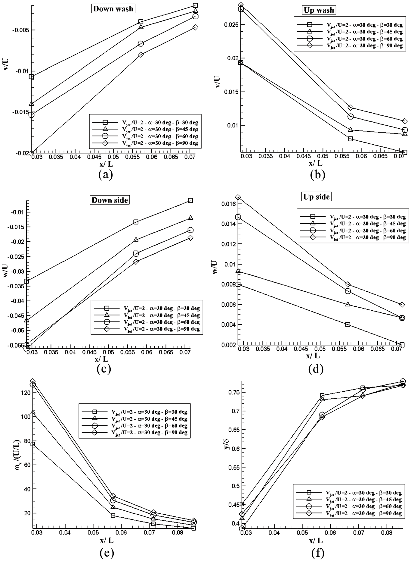
As shown in Figure 12, the maximum vortex velocity in the y and z directions was generally reduced in areas farther from the edge of the microjet. It is also observed that a larger $β$ led to higher velocities. However, the maximum velocity changed by choosing $β$ in the range from 60° to 90°. For smaller angles and at a distance from the edge of the microjet, the location of the maximum velocity was no longer observable as the vortex dissipated more rapidly. The microjet strength was reduced at points farther from the edge of the microjet. This reduction was nonlinear and the gradient slope was gradually decreased. Furthermore, for $β$ angles wider than 60°, the variations were not substantial. Therefore, $β$ can be chosen in the range from 60° to 90°. These settings made for a stronger microjet compared with microjets at other angles, and hence led to a more stable vortex. The boundary layer graph also indicates that the vortex remained in the boundary layer. Nevertheless, at locations farther from the edge of the microjet, the vortex became weaker and more expanded. Therefore, its top edge moved out of the boundary layer almost linearly.

Figure 12.

Results for variable β, VR = 1, and α = 30°: (a) v for the downwash, (b) v for the upwash, (c) w for the down side, (d) w for the up side, (e) maximum ωx, and (f) distance of up side vortex from the boundary layer.

Results for variable $β$ , VR = 1, and $α = 45 °$

As shown in Figure 13, this section evaluates the effect of variations in $β$ on vortex strength and location by considering the VR and $α$ as constants. The general trend for $α = 45 °$ is similar to that for $α = 30 °$ . However, the velocity in the y and z directions and the vortex strength were reduced. In fact, vortex strength decreased by 7% with respect to the case with $α = 30 °$ at the beginning of the flow. However, at points farther from the edge of the microjet, both cases led to similar vortex strengths. Despite the fact that the vortex remained within the boundary layer, it became closer to the edge of the boundary layer compared with the case with $α = 30 °$ . As a result, its effect on the surface flow diminished. According to the graphs, $β$ ranging from 60° to 90°, similar to the previous case, led to generally more favorable results. However, $β = 90 °$ provides better results than $β = 60 °$ .

Figure 13.

Results for variable β, VR = 1, and α = 45°: (a) v for the downwash, (b) v for the upwash, (c) w for the down side, (d) w for the up side, (e) maximum ωx, and (f) distance of up side vortex from the boundary layer.

Results for variable $β$ , VR = 1, and $α = 60 °$

For this case, it was not possible to provide a velocity graph or vortex locations due to the reduction in velocity and [more rapid] vortex dissipation compared with previous cases. However, Figure 14 on the vortex indicates a trend similar to the previous cases with smaller $α$ . The wider angle in the present case led to a considerable reduction in vortex strength and its rapid dissipation. As shown in the figure, the maximum vortex strength was reduced by 44% with respect to the case with $α = 30 °$ . It is observed that in the present case, wider $β$ angles also led to better results. Moreover, the graphs indicate that smaller $α$ could provide better results.

Figure 14.

Results for variable β, VR = 1, and α = 60°: (a) maximum ωx and (b) distance of up side vortex from the boundary layer.

The results for VR = 1 and different values of $α$ show that the best vortex due to the microject was generated with $β$ ranging from 60° to 90°. $β$ was set equal to 60° in further analyses, where variations of the other parameters were studied. It was also found that lower values of $α$ could lead to better results. However, for even smaller surface angles, the flow from the microjet was so close to the bottom of the channel that it had such undesirable effects as microjet energy loss and deviation of flow direction, rendering accurate experimental measurements very difficult or impossible. Considering the small difference between the results for $α = 30 °$ and $45 °$ , it can be concluded that the results will not change substantially for $α < 60 °$ . Therefore, $α$ was set equal to 30° in the next stages of the analysis.

Results for variable $β$ , VR = 2, and $α = 30 °$

Based on the previous results, this section evaluates microjet effects by varying $β$ and choosing $α = 30 °$ and VR = 2. The aim was to assess how the appropriate value for $β$ changed at higher velocities. A trend similar to that of the cases with VR = 1 was observed as shown in Figure 15. As the microjet velocity increased, the velocity along the y and z directions and the vortex strength grew sharply. The vortex in this case also remained within the boundary layer, and was about 350% stronger than that in the case with VR = 1. However, as the vortex persisted at a farther distance from the edge of the microjet and dissipated more slowly, the variations in the far-field were different from that of the case with VR = 1. The ratio of variations of vortex-to-bottom distance to the boundary layer was nearly constant in the present case, which means that the vortex was affected by the boundary layer and pushed out of it. In fact, while at the start of the movement, the increased rate of the distance between the top edge of the microjet and the bottom was larger with respect to the boundary layer, it was reduced as the vortex moved under the influence of the boundary layer. It is observed from the graphs that VR = 2 also resulted in the angles from 60° to 90° to be the best range for $β$ .

Figure 15.

Results for variable β, VR = 2, and α = 30°: (a) v for the downwash, (b) v for the upwash, (c) w for the down side, (d) w for the up side, (e) maximum ωx, and (f) distance of up side vortex from the boundary layer.

Results for variable $β$ , VR = 4, and $α = 30 °$

Based on the previous results, this section evaluates microjet effects by varying $β$ and choosing $α = 30 °$ and VR = 4. A trend similar to that of the cases with VR = 1 was observed as shown in Figure 16. As the microjet velocity increased, the velocity along the y and z directions and the vortex strength grew sharply. The vortex was about 680% and 85% stronger than the vortices with VR = 1, and 2, respectively. This means that as the velocity increased, the positive slope of the increase in the vortex strength dropped. Therefore, the effect of a raise in microjet velocity larger than a certain value became negligible. The vortex in this case also remained within the boundary layer. The ratio of variations of vortex-to-bottom distance to the boundary layer also remained nearly constant in the present case for angles wider than a certain value. As the graphs show, VR = 4 also resulted in angles from 60° to 90° to be the best range for $β$ . However, at higher VRs, smaller $β$ angles led to better results. In the present case, there was a 1.2% difference between the results with $α = 60 °$ and those with $α = 90 °$ , and an 8.4% difference between the results with $α = 45 °$ and those with $α = 90 °$ .

Figure 16.

Results for variable β, VR = 4, and α = 30°: (a) v for the downwash, (b) v for the upwash, (c) w for the down side, (d) w for the up side, (e) maximum ωx, and (f) distance of up side vortex from the boundary layer.

Results for variable $α = 30 °$ , $β = 60 °$ , and VR = 4

A discussion was presented in the introduction on the formation of a strong vortex from a vortex pair. This phenomenon is illustrated in Figure 17 for $α = 30 °$ , $β = 60 °$ , and VR = 4. It is observed that the counter-rotating vortices are formed near the microjet. The vortex whose center was closer to the surface gradually weakened and, due to the diminished strength and heightened pressure, the smaller vortex was absorbed by the larger one, both forming into a single dominant vortex.

Figure 17.

Contours of the formation of a single dominant vortex from the initial vortex pair for α = 30°, β = 60°, and VR = 4.

The formation of the dominant vortex and its complete dissipation are illustrated in Figure 18 for variable $β, α = 30 °$ , and VR = 4. It is observed that increasing $β$ caused the location of the vortex formation to move closer to the microjet. Increasing the angle larger than a certain value, however, did not bring about any substantial change. It is worth noting that at lower microjet velocities the vortex formation location was so close to the microjet that the formation stages were impossible to distinguish. In fact, higher velocities resulted in the vortex to form at farther distances. The final location at which a complete vortex could be observed was more distant for larger $β$ . However, variations of the formation location decreased as the angle became wider. As the previous results indicated, for the VRs = 1, 2, and 4, x/L was 0.058, 0.078, and 0.18, respectively.

Figure 18.

The position of altering of the main counter-rotating vortex pair into a single dominant vortex.

Figure 19 presents the results contours for $α = 30 °$ , $β = 60 °$ , and VR = 4, at various distances. The contours show that the vortex was formed and absorbed to the right side due to the microjet angle. After a certain distance from the edge of the microjet, the main flow dominated, causing the vortex move only toward the tunnel outlet. The figure also indicates that the vortex was gradually detached from the surface and moved upwards. Due to the vortex strength dissipation and the boundary layer growth, the vortex did not move out of the boundary layer. The contours also show the position of the maximum velocity along the y and z directions. The boundary layer was affected particularly near the microjet due to its location and orientation. The microjet with a small diameter still had a considerable effect on the boundary layer at x = 0.6 m

Figure 19.

Results for variable β, VR = 4, and α = 30°: (a) ωx v for the downwash, (b) streamlines, (c) v, (d) w, (e) u, and (f) boundary layers.

Considering the position of the center, left side, and right side of the vortex, the velocity variations along the x, y, and z-directions for various distances along the x-axis are shown in Figure 20 for the center, left side, and right side of the flow. The graph shows the difference in flow velocities between the cases with and without a microjet. It is also possible to determine the position of the boundary layer from the presented graphs. The effect of the microjet gradually decreased at distances farther from its edge. Therefore, the results followed those of the case without a microjet more closely. The graph of the velocity along the x direction shows that u for the upwash and downwash flows near the bottom wall was lower and higher, respectively, than the velocity in the center. This difference in velocities is due to the fact that the vortex rotation axis was at an angle to the x axis. As the distance across the two walls became wider, the velocity in the y direction gradually increased downstream. v was observed to increase linearly in the y direction at any cross section along the x axis. Adding the microjet to the flow caused the velocity variations to occur almost equally for the upwash and downwash flows. Moreover, the distance from the lower and upper points of the vortex to the bottom can be determined by observing maximum w. The graph shows that the vortex gradually expanded. In fact, the maximum movement of the upper portion of the graph in the y direction was larger than that of the lower portion.

Figure 20.

Variations of u, v, and w in the center, downwash, and upwash flows in the vortex for α = 30°, β = 60°, and VR = 4 (numerical data).

Reynolds stresses for variable microjet

Based on the previous results, this section provides an analysis of the Reynolds stresses using the selected microjet specifications. Reynolds stresses u′u′, u′v′, and u′w′ are presented for VR = 1, 2, and 4, and $β$ = 60° and 90°, with $α = 30 °$ , at various sections for the center, upwash, and downwash flows in the vortex. Figures 21 to 23 show that velocity fluctuation v′ was always in the opposite direction to velocity fluctuation u′. The velocity fluctuations gradually became less severe as the flow moved downstream. This reduction in velocity fluctuations, which was more pronounced for larger VRs and in the graphs showing w′, can be explained by the observation that as the flow moved farther from the microjet, it continued to experience velocity variations along the x direction due to the wall. The velocity variations also persisted in the y direction due to the distance across the walls of the wind tunnel becoming wider. However, there were no substantial flow variations along the z axis. Therefore, velocity variations along the z axis decreased downstream. The graphs also indicate that w′ experienced a larger increase in the upwash and downwash flows than in the center. Moreover, as the VR increased, the increase in the Reynolds stress w′ was higher than the increase in v′, while the corresponding increase in v′ was higher than that in u′. As mentioned above, the factors stimulating turbulence were stronger along the x and y directions than the z direction. Therefore, the same turbulence-stimulating factors of the main flow were dominant in the x and y directions, even after the microjet was added. However, the added microjet was the dominant contributing factor to turbulence along the z axis. The maximum change in the Reynolds stress along the x direction with the VR between 1 and 4 was 10% when the microjet was used. The corresponding values along the y and z directions were about 15% and 270%, respectively. Furthermore, almost similar trends were observed in the variations of the Reynolds stress between 60° and 90° angles. However, the Reynolds stress was larger for $β = 90 °$ than that for $β = 60 °$ . This difference grew as the velocity increased.

Figure 21.

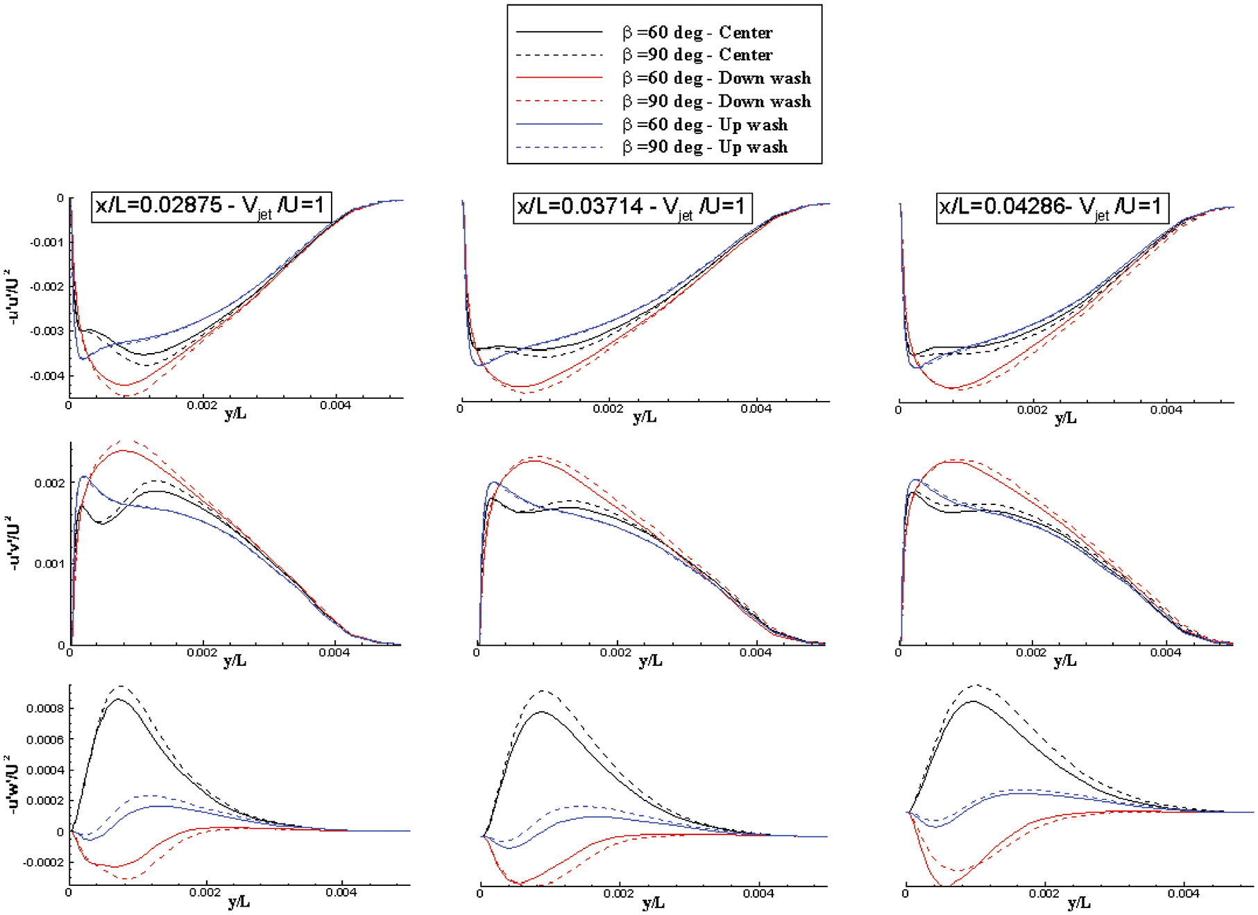
Variations of u′u′, u′v′, and u′w′ in the center, downwash, and upwash flows in the vortex for α = 30°, β = 60°and 90°, and VR = 1 (numerical data).

Figure 22.

Variations of u′u′, u′v′, and u′w′ in the center, downwash, and upwash flows in the vortex for α = 30°, β = 60°and 90°, and VR = 2 (numerical data).

Figure 23.

Variations of u′u′, u′v′, and u′w′ in the center, downwash, and upwash flows in the vortex for α = 30°, β = 60°and 90°, and VR = 4 (numerical data).

Conclusion

The effects of the ratio of microjet to wind tunnel inflow velocity and microjet angles $α$ and $β$ on the strength of the generated vortex were analyzed. The analysis was carried out for VRs = 1, 2, and 4, $α$ = 30°, 45°, and 60°, and $β$ = 30°, 45°, 60°, and 90°. The best microjet specifications were finally determined by categorizing and analyzing the results.

The results showed that the vortex was more stable at higher velocities. In fact, at VRs = 1, 2, and 4, the x/L (The length which the longitudinal vortex retains in the flow) values were 0.058, 0.078, and 0.18, respectively. Compared to VR = 1, the vortex strength for VRs = 2 and 4 grew by 350% and 680%, respectively.

The best microjet angles at various velocities were found to be about $α = 30 °$ , and the range $β = 60 °$ to 90°. Moreover, as the VR increased, in different angles vortices were formed similar strength.

While a wider $β$ angle caused the dissipation location of the weak vortex move closer to the microjet, increasing it greater than a certain value did not change it substantially. Furthermore, at lower microjet velocities, the formation location of the dominant vortex was so close to the microjet that the formation stages were impossible to tell apart.

As $β$ increased, total dissipation of the vortex occurred farther from the microjet. However, increasing $β$ greater than a certain value did not have a considerable effect on the dissipation location. Higher velocities also caused the location of the total vortex dissipation occur at a larger distance to the microjet.

Due to the microjet, free flow velocity, and the bottom wall, the generated vortex were moved along the positive z, x, and y axes, respectively. However, at locations farther than a certain distance from the microjet, the effect of the microjet on the vortex became negligible. The vortex remained inside the boundary layer for all cases.

Velocity fluctuations gradually decreased downstream, which was more noticeable for larger VRs and in the graphs showing w′.

By adding the microjet to the flow, the highest variation in the Reynolds stress along the x direction from VR = 1–4 was 10%. The corresponding values along the y and z directions were 15% and 270%, respectively. Velocity fluctuations gradually decreased downstream, which was more noticeable for larger VRs and in the graphs showing w′. Moreover, $β = 60 °$ and 90° resulted in almost similar Reynolds stresses.

Footnotes

Appendix

Declaration of conflicting interests

The author(s) declared no potential conflicts of interest with respect to the research, authorship, and/or publication of this article.

Funding

The author(s) disclosed receipt of the following financial support for the research, authorship, and/or publication of this article: This project is funded by SXIT - Grant number: in 2019(Gfy19-01).

ORCID iD

Mohammad Javad Pour Razzaghi

Author biographies

Mohammad Javad Pour Razzaghi received the B.Sc. and M.Sc. degree in mechanical engineering from the Ferdowsi University of Mashhad, Iran, in 2011 and 2015 respectively. He currently works as a Ph.D. candidates at school of mechanical engineering in Nanjing university of science and technology, China. His current research interests include the computational fluid dynamics and flow control techniques.

Dr. Cheng Xu is a full professor at Mechanical Engineering school at Nanjing University of Science and technology. His research interests lie in the fields of separation flow control, Impact dynamics and Products design method.

Yue Liu received the Ph.D. degree in mechanical engineering from the Nanjing university of science and technology, China, in 2018. He currently works as a college lecturer at school of aeronautics and astronautics in ShaanXi institute of technology, China. His current research interests include the turbulence and flow control techniques.

Yasin Masoumi received the M.Sc. degree in mechanical engineering from Shiraz University of Technology, Iran, in 2018. Iran University of Science and Technology, where he is currently pursuing the Ph.D. degree in Acoustics Research Laboratory. His current research interests include vortex shedding, FSI problems, piezoelectric materials, and flow control techniques.

References

Lefebvre

. Investigation of co-flow jet flow control and its applications. Thesis, University of Miami, 2015.

Anderson

JJFoa

. Introduction to the fundamental principles and equations of viscous flow. 3rd ed. New York, NY: McGraw-Hill, 2001, pp.713–744.

Raman

. Numerical investigation of vortex generators and jet in cross-flow enhancements. Doctoral Thesis, The University of Texas at Arlington, 2016.

Pearcey

HJBl

and control f. Shock induced separation and its prevention. Boundary layer and flow control 1961; 2: 1170–1344.

PourRazzaghi

. Numerical study of minute vortex generator jets in a turbulent boundary layer. J Phys Conf Ser 2020; 1507; 082011.

Johansen

. Numerical simulations of turbulent flows. Theses and Dissertations, Carleton University, 2005.

Iuso

Vigevano

Scialabba

. Effects of injector geometry in air-jet vortex-generator flow control. Master Thesis, Institute of Aerodynamics, 2018.

McCurdy

WJUAC

. Investigation of boundary layer control of an NACA 16-325 airfoil by means of vortex generators. Research Department, Rept. M-15038, 1948, 3.

Wallis

. The use of air jets for boundary layer control. Australia: Aeronautical Research Labs Melbourne, 1952.

10.

Rixon

Johari

HJJFE

. Development of a steady vortex generator jet in a turbulent boundary layer. J Fluids Eng 2003; 125: 1006–1015.

11.

Ortmanns

Kähler

CJIjoh

flow

. The effect of a single vortex generator jet on the characteristics of a turbulent boundary layer. Int J Heat Fluid Flow 2007; 28: 1302–1311.

12.

Von Stillfried

Wallin

Johansson

, et al. Evaluation and parameterization of round vortex generator jet experiments for flow control. AIAA J 2012; 50: 2508–2524.

13.

Lasagna

Orazi

Iuso

GJFDR

. Streamwise vortices originating from synthetic jet–turbulent boundary layer interaction. Fluid Dyn Res 2013; 46: 015501.

14.

Feng

Y-Y

Song

Y-P

Breidenthal

REJAJ

. Model of the trajectory of an inclined jet in incompressible crossflow. AIAA J 2018; 56: 458–464.

15.

Beresh

Henfling

Spillers

, et al. Influence of the fluctuating velocity field on the surface pressures in a jet/fin interaction. J Spacecraft Rockets 2018; 55: 1098–1110.

16.

Alimi

Wünsch

OJF

. Numerical investigation of steady and harmonic vortex generator jets flow separation control. Fluids 2018; 3: 94.

17.

Szwaba

Flaszynski

Doerffer

PJCJoA

. Streamwise vortex generation by the rod. Chin J Aeronaut 2019; 32: 1903–1911.

18.

Liu

Zhang

Liu

PJAiME

. Flow control in supersonic flow field based on micro jets. Adv Mech Eng. Epub ahead of print 22 January 2019. DOI: 10.1177/1687814018821526.

19.

Masumi

Nikseresht

AHJAOR

. Comparison of numerical solution and semi-empirical formulas to predict the effects of important design parameters on porpoising region of a planing vessel. Appl Ocean Res 2017; 68: 228–236.

20.

White

Corfield

. Viscous fluid flow. New York, NY: McGraw-Hill, 2006.

21.

Davidson

. An introduction to turbulence models. Sweden: Chalmers University of Technology, 2015.

22.