Sage Journals: Discover world-class research

Abstract

Semi-built-up crankshafts are universally manufactured by shrink-fitting process with induction heating device. The configurations of induction coil have a great impact on the distributions of eddy current and temperature of crankthrows. Most induction devices are apt to cause some undesirable phenomena such as uneven temperature distribution and irregular deformation after induction heating. This article proposes a modified configuration of induction heating coil according to the crankthrow geometry. By combining the heat conduction equation and the heat boundary conditions, a three-dimensional finite element model, which takes into account the nonlinearity of the material’s electromagnetic and thermal physical properties in the heating process, was developed. The influence of several parameters, such as position and curvature of the arc coil, the current frequency and density, coaxiality of crankweb hole and coil, influencing the temperature distribution inside the crankthrow was also analyzed. The comparison with the numerical simulation results of the original configuration indicates that the modified configuration has better adaptability to the crankthrow. Also, it can help to improve the temperature distribution, and reduce the deformation of the shrink-fitting hole. This exploration provide an effective way for the enterprise to further enhance the shrink-fitting quality of crankshaft.

Keywords

Induction coil configuration semi-built-up crankshaft shrinking fitting thermal distribution

Introduction

In recent years, with development of global economy and trade, large-scale and intensive ocean vessels are becoming an inevitable trend. As the key component of super-large-scale marine low speed engine, semi-built-up crankshafts, as shown in Figure 1, are subjected to bending moment, torsion and complex alternating loads reaching hundreds of tons.¹

Figure 1.

W12X92 semi-built-up crankshaft of low-speed 2-stroke marine diesel engine.

The semi-built-up crankshaft is a complex mechanical system interconnected by shrink-fitting parts called journals to other parts called crankthrows.² The quality of the joint depends on the distribution of its interference. If the deformation of the crankweb hole is out of tolerance after heated, the joint is apt to be poorly mounted and the strength of connection is insufficient owing to the uneven distribution of the assembly interference. Moreover, all the journals are in misalignment after complete assembly. Under complex loading conditions, crankshafts will result into fatigue phenomena, such as fretting wear, fatigue crank, and fatigue fracture with a stress much lower than that required to cause fracture. It was pointed that about 85% of the quality problems of large marine crankshafts are caused by fatigue problems.³

Therefore, the quality and life of the semi-built-up marine crankshaft are partially dependent on the shrink-fitting process.⁴ However, the problems of what kind of heating device to use, how to get a more uniform temperature distribution and how to control the irregular deformation in the process of induction heating are far from enough by experience. In order to fulfill design requirements of semi-built-up marine crankshaft, manufacturers have to take lots of time and resources to do superfluous tests. Therefore, designing an induction heating device capable of streamlining the shrink-fitting process is essential for further improving the manufacturing efficiency and product quality of the new generation of super-large-scale marine crankshafts such as G95 and X92.

In the traditional shrink-fitting process, gas-fuel heating is the most widely employed method by most manufacturers.^5,6 During heating process, the flame contacts the crankweb directly. Therefore, this method is time consuming, and the thermal deformation of workpiece is difficult to control. Also, the epidermis of the heated portion is easy to be oxidized and carbonized. Different from gas-fuel heating, induction heating^7,8 is a non-contact heating method and has advantages of fast heating speed, low energy consumption, small material burning loss, less surface oxidation, easy controllability, etc. It has been gradually adopted by manufacturers and become quite popular these years in industry.^9–13 However, there are few publications on this topic of assembled marine crankshafts. Zhang et al.¹⁴ and Fu et al.¹⁵ established three-dimensional finite element models, including the induction coil, crankthrow, and air, to numerically simulate the distribution of temperature during the period of induction heating with software ANSYS. Zhang et al.¹⁶ adopted the non-dominated sorting genetic algorithm (NSGA-II) within an optimization software iSIGHT to get the optimal input parameters of an induction heat treatment apparatus.

Induction heating is a complex process. The configuration, position, and other parameters of the induction coil have an important influence on eddy current distribution, temperature distribution, electromagnetic distribution, and thermal assembly quality of the crankshaft. At present, it is difficult to describe this process accurately and completely with mathematical equations. Recently, the finite element method has been used extensively in many problems associated with electro heat applications such as induction heating. The numerical calculation of induction heating has become increasingly common. Cho¹⁷ established a coupled electro-magnetic and thermal model for numerical analysis of an induction heating system, highlighting the dynamic effect of the workpieces moving relative to the inductors. Li et al.¹⁸ used the finite element method to build a single coil induction hardening model, and attained temperature curves on the surface region of a ball screw by numerical simulation. Han et al.¹⁹ carried out finite element numerical computation and comparative analysis for sprocket heating processes between circular coil and profile coil, respectively. Naar and Bay²⁰ tested zero- and first-order algorithms and coupled with 2D and 3D multi-physics finite element models for induction heat treatment problems.

Considering the structure of crankthrows, this paper intends to (i) design an arc-shaped induction coil, (ii) develop a coupled electro-magneto-thermal finite element model for numerical analysis of induction heating process, which is related to current density and frequency, heating time and other parameters, (iii) integrate with the heat conduction equation and the thermal field boundary conditions to solve the given model and get more acquainted with the evolution of the internal thermal distribution of the workpiece, and (iv) clarify the effects of the configuration and position of the induction coil, current frequency and density, and coaxiality on the thermal distribution of the crankthrow and its adaptability.

Configuration description

Crankthrow induction heating is a complex process including electromagnetic, thermal and metallurgic phenomena. Firstly, industrial power with frequency of 50 Hz needs to be converted into constant direct current (DC) through rectifier circuit, then DC is converted into alternating current (AC) with frequency required by induction heating by inverter, and then AC is sent to induction coil through transformer. The process is shown in Figure 2. As the internal heat source, the eddy Joule heat produced by the workpiece will be used as the heat source for the heat conduction process. Therefore, the currents loaded on the coils will directly affect the electromagnetic induction process, which will greatly affect the heating of the workpiece.

Figure 2.

Flow chart of current conversion.

The coils generate alternating magnetic fields, in which the induction crankthrow is immersed. As a consequence, the induction crankthrow is heated by means of eddy currents and magnetic hysteresis. The induced eddy currents generate energy in the form of heat, which is then distributed throughout the workpiece. Joule heat is the main part before the workpiece temperature reaches Curie temperature. In addition, the thermal effect caused by hysteresis will also provide a small part of heat.

As the quality of the joint depends on its interference and on the internal stresses generated during the cooling process, the crankweb hole should be heated to form a relatively uniform temperature field to meet the accuracy requirements of the crankshaft after shrink fitting. However, experimental investigations and practical applications show that the induction heating system with a separate structure consisting of a rectangular coil and a circular coil, as shown in Figure 3, is lack of flexibility and robustness to different crankthrows and usually causes irregular deformation induced by non-uniform thermal temperature. In order to enhance the heater’s versatility, the coils should have a certain flexibility. Coupled with the requirements of thermal uniformity and assembly operation, the coil is not suitable for an integrated configuration design.

Figure 3.

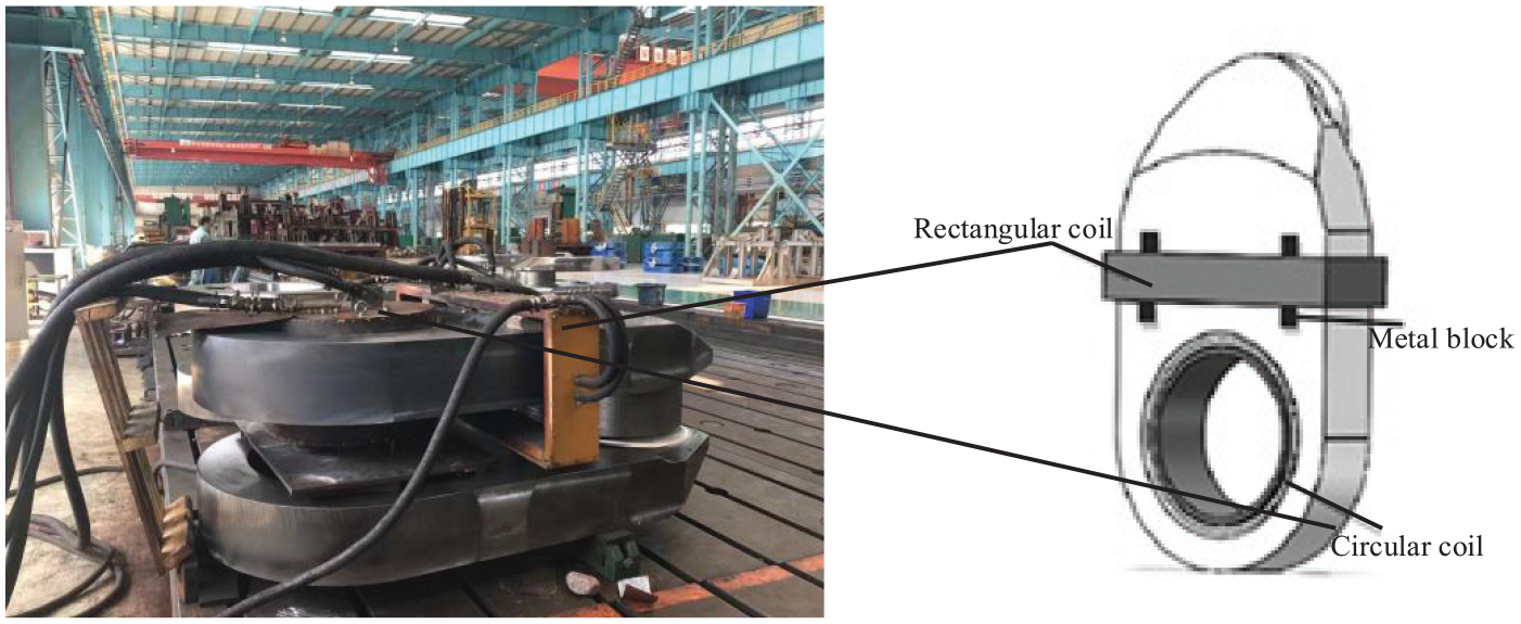
Typical induction heating system layout for crankshaft thermal shrink fitting.

Referring to the typical configuration (shown in Figure 3), the induction heating coil is still designed as a separate-type configuration. Figure 4(a) and (c) denote the sematic diagrams of the arc coil and circular coil respectively. As shown in Figure 4(d), the circular heating coil is still located in the crankweb hole and an arc one between the crankweb hole and the crankpin. The arc coil and circular coil are concentric with the crankweb hole. The relative position between the arc coil, circular coil, and crankthrow is kept constant by adding some identical metal blocks. Figure 4(b) shows that the cross-section of arc coil and the wire inside is wound by winding.

Figure 4.

The modified coil configuration. (a) Arc coil. (b) Cross-section of the arc coil. (c) Circular coil. (d) System layout.

Finite element model

FEM details

The mechanical parameters of the crankthrow material change with temperature. The variation of temperature leads to the coupling of electromagnetic field and temperature field. In order to get accurate numerical results, it is necessary to take consideration of thermal-physical properties of the selected material in the early electromagnetic simulation process. The temperature-dependent mechanical properties and thermal-physical parameters of the selected steel S34MnV are given in Table 1. It’s Poisson’s ratio µ = 0.3, thermal emissivity of the crankthrow surface ε = 0.68.

Table 1.

Mechanical and thermal-physical properties of S34MnV under different temperatures.

Temperature/°	Density/kg·m⁻³	Elastic modulus/GPa	Thermal conductivity /W·(m·K)⁻¹	Specific heat capacity /J·(kg·K)⁻¹	Resistivity/(Ω·m)	Relative permeability
20	7799	213	41.7	464	1.9 × 10⁻⁷	200
100	7780	211	40.3	505	2.5 × 10⁻⁷	197
200	7751	204	38.8	546	3.4 × 10⁻⁷	194
300	7717	197	36.8	589	4.4 × 10⁻⁷	180
400	7678	190	33.7	635	5.5 × 10⁻⁷	170
500	7642	183	30.9	686	6.5 × 10⁻⁷	157

In electromagnetic field analysis, the outmost surface of the air domain approximately meets the parallel boundary conditions of the magnetic field lines. Therefore, the magnetic potential can be set to zero. For other positions, the vertical boundary conditions of the magnetic field lines are naturally satisfied. In temperature field analysis, the initial crankthrow and environment temperature are 20°. In stress–strain field analysis, since the crankthrow is located on the ground and there is no normal displacement at each node close to the ground, the normal displacement constraint with zero is applied in this direction. At the same time, the displacement constraints in x, y, and z directions should be applied to the center point of the plane to avoid non-convergence during numerical calculation. In addition, the crankthrow has a symmetric structure, and the boundary condition of U__x = 0 must be satisfied on the plane of symmetry.

The FEA was performed in the ANSYS Software. The mesh represents only the half of the geometry of crankthrow (Figure 5(a)). Utilization of the symmetry boundary conditions makes it possible to obtain more accurate analysis because of the higher number of finite elements in the half-model mesh.²¹ As illustrated in Figure 5(a), the grid density decreases from the outmost surface to the center, and finer mesh can be seen around the crankweb hole. For electromagnetic field analysis, the induction coil, crankthrow and air can be meshed with SOLID117 element. When performing the temperature field analysis, the element type SOLID90 can be used for the crankthrow FEA model, and the SOLID95 element for the structural field analysis.

Figure 5.

(a) Finite element mesh of the crankthrow (the half-model with geometric symmetry). (b) Air domain surrounding the induction target. (c) Current-source excitations for the induction heating coils.

In this study, MAXWELL, a premier electromagnetic field simulation module of ANSYS software, was used to predict the power densities and temperature distribution of crankthrow. The modeling domain must be truncated to some finite size that will give reasonably accurate results but will not require too much computational effort to solve. As illustrated in Figure 5(b), we established the air domain surrounding the induction target as a cylinder with radius 6 m and height 10 m. Figure 5(c) shows the current-source excitations for the induction heating coils.

Figure 6 shows the coupled electro-magneto-thermal analysis flowchart of crankthrow. Firstly, according to the initial temperature distribution of the crankthrow, the physical parameters of the material are determined and applied to the solution of the electromagnetic field calculation, and the heat flux that the electromagnetic field output is obtained. Then the heat flux is input as the internal heat source parameter of the thermal field, and perform the temperature field calculation. At the same time, the material physical parameters are updated with respect to the temperature distribution of the crankthrow and the electromagnetic field is computed. This iteration is continued until the heating cycle ends.

Figure 6.

The coupled electro-magneto-thermal analysis flowchart of crankthrow.

Temperature distribution and thermal deformation

The cross-sectional area of the circular coil is 1.17 × 10⁻² m² (A₁), and that of the rectangular and arc coils is 8.1 × 10⁻³ m² (A₂), respectively. Turns of the circular coil is 80 (n₁) and the current in each single-turn is 180 A (I₁). Turns of the rectangular and arc coils are defied as 67 (n₂), and the single-turn current is 80 A (I₂). The harmonic frequency of circular, rectangular and arc coil current is 1000 Hz.

Figure 7 presents temperature distribution of the crankthrow heated by the original and modified configuration for 5 h, respectively. It can be found from qualitative observation of the 3D temperature field of the crankthrow that, the highest temperature is reached in the surface layer of crankweb hole under the original coil configuration, and the value is 377.55°C. The lowest point is laid on the outermost surface and the value is 329.4°C. The maximum temperature difference is 48.15°C. However, within the same time, the highest and lowest heat treatment temperatures are 343.07°C and 321.2°C respectively. The maximum deviation of heat treatment temperature of the crankthrow is 21.87°C. In this condition, the temperature distribution is closely associated with the spatial distribution of magnetic induction lines during heating. For the modified coil configuration, a certain amount of magnetic induction lines are distributed along the wall of the crankweb hole, which has positive significance for uniform distribution of energy.

Figure 7.

Contour plots of temperature distribution under different coil configurations. (a) Original configuration. (b) Modified configuration.

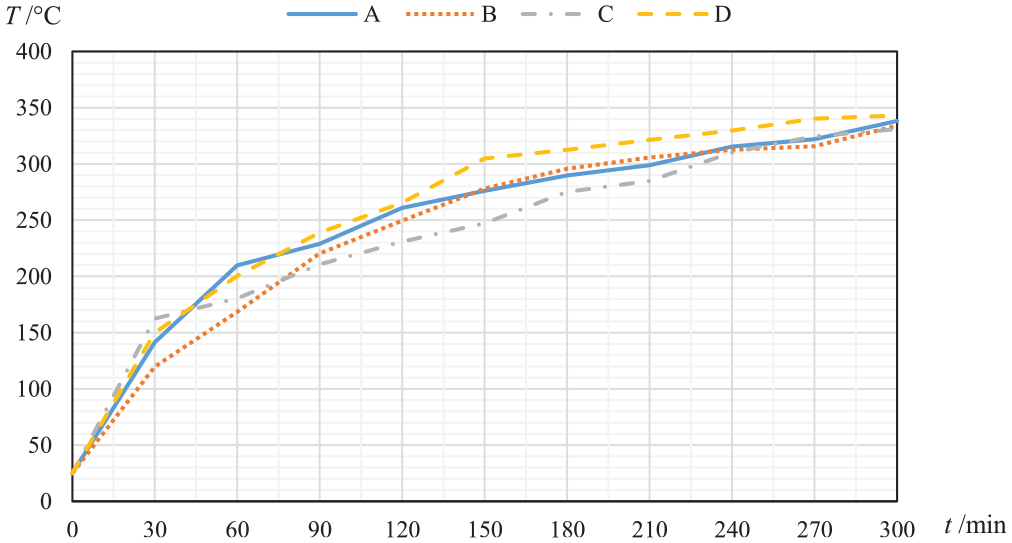
Figure 8 presents four points denoted as A, B, C, and D on the surface of the crankweb hole for the observation of temperature variation. The origin of the coordinates is set to the center of the crankweb hole near the ground. x represents horizontal radial and y represents vertical radial. From Figure 8, it can be seen that points A and B are rightmost endpoints on the surface of the crankweb hole. Points C and D are located on the edge of the crankweb hole along Y-axis. The evolutions of the corresponding temperatures with time before and after the modification are shown in Figures 9 and 10.

Figure 8.

Location diagram of the observation points on the crankweb hole.

Figure 9.

Temperature evolution of the observation points heated by the original configuration.

Figure 10.

Temperature evolution of the observation points heated by the modified configuration.

From the view of variations in the slope of the curve, during the first 5 h of heating, the rate of temperature increase is significantly faster within about 30 min than the subsequent time, and the crankthrow temperature became stable after 5 h. The reason is that a more stable temperature gradient is generated inside the crankthrow during heating. The heat is transferred from the high temperature to the low temperature, so that the speed of temperature decreases. After 5 h heat treatment with the original configuration, the crankthrow attains the highest temperature at 377.55°C, the lowest temperature at 340.15°C, and the temperature difference ΔT_b = 37.4°C among the four points around the crankweb hole, and the highest temperature yielded by the modified configuration is 343.07°C, the lowest temperature is 330.92°C, and the temperature difference ΔT_a is 12.15°C. It can be seen that the temperature difference around the crankweb hole is significantly reduced, and the uniformity of temperature distribution is better improved.

Coupled with the electromagnetic-thermal analysis, structural finite element analysis was carried out with ANSYS software. The displacement changes at various points on the crankthrow were recorded during 5 h of induction heating. The results are given in Figure 11.

Figure 11.

Total deformation of the crankweb.

The axial displacement tables are derived from the structural field analysis results. Tables 2 and 3 present the crankweb linear displacement distributions in x and y directions, respectively. b_x and b_y are displacement results obtained by the original configurations, and a_x and a_y are displacement results obtained by the modified configuration.

Table 2.

Linear displacement of the crankweb in x direction.

x direction/mm	b_x/mm	a_x/mm
−850	−0.965	−0.947
−782.17	−0.912	−0.924
−711.33	−0.871	−0.912
−640.5	−0.835	−0.899
−569.67	−0.812	−0.893
569.67	0.812	0.893
640.5	0.835	0.899
711.33	0.871	0.912
782.17	0.912	0.924
850	0.965	0.947

Table 3.

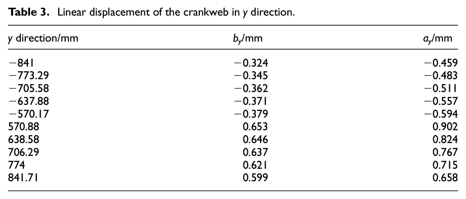
Linear displacement of the crankweb in y direction.

y direction/mm	b_y/mm	a_y/mm
−841	−0.324	−0.459
−773.29	−0.345	−0.483
−705.58	−0.362	−0.511
−637.88	−0.371	−0.557
−570.17	−0.379	−0.594
570.88	0.653	0.902
638.58	0.646	0.824
706.29	0.637	0.767
774	0.621	0.715
841.71	0.599	0.658

From Table 2, it can be seen that the linear displacement in x direction is symmetrically distributed. The reason is that the crankthrow is a left-right symmetrical structure. The maximum and minimum linear displacements in x direction for the modified and original configurations are 0.947, 0.965, 0.893, and 0.812 mm respectively. The maximum linear displacement is close to the side surface of the crankthrow in x direction. It is caused by no external constraints, which is consistent with the theory. The maximum linear displacement differences yielded by the modified and original configurations on the crankweb hole in x direction are 1.785and 1.623 mm, respectively.

It can be seen from Table 3 that the closer to crankpin, the smaller the linear displacement in y direction is. The reason is that crankpin is non-heating area and the temperature is low and the thermal deformation is small. The maximum linear displacement yielded by the modified configuration appears on the inside of the crankweb hole with a value of 0.902 mm. The maximum linear displacement yielded by the original configuration appears directly below the crankweb hole with a value of 0.653 mm. The maximum linear displacement differences on the crankweb hole in y direction are 1.496 and 1.032 mm respectively.

Difference between maximum diameter and minimum diameter of the crankweb hole after induction heating using the modified and original configurations are 0.29 and 0.59 mm, respectively. It can be seen that the roundness of the crankweb hole has been greatly improved.

Influencing parameters

Position

The four-point temperature distributions on the crankweb hole can be attained by changing location of the arc coil while keeping the other parameters identical. d represents the distance from the inner circle point of the arc coil to the center of the crankweb hole, which is shown in Figure 12. Figures 13 and 14 show the temperature evolutions of the observation points when d = 900 and 800 mm respectively.

Figure 12.

Arc coil location.

Figure 13.

Temperature evolution of the observation points when d = 900 mm.

Figure 14.

Temperature evolution of the observation points when d = 800 mm.

The linear displacement with biggest value is close to the side surface of the crankthrow in x direction. When d = 900 mm and d = 800 mm, the maximum linear displacement differences on the crankweb hole in x direction is 1.912 and 1.969 mm, respectively. The closer to the position of crankpin, the smaller the linear displacement is in y direction. This is because that crankpin is a non-heating area and the temperature is low and the thermal deformation is small. The maximum linear displacement differences on the crankweb hole in y direction are 1.473 and 1.358 mm, respectively.

From the above, we can know that when the positions of the arc coil d are 1000, 900, and 800 mm, differences between maximum diameter and minimum diameter of the crankweb hole after heating by the modified configurations are 0.29, 0.44, and 0.61 mm, respectively. It can be seen that the minimum difference of the shrink-fitting hole is at d = 1000 mm, but this distance cannot be increased due to the structure of the crankthrow.

Curvature

Changing the radius of the arc coil and making the distance from the farthest point of the coil to the center of the crankweb hole constant (shown in Figure 15), it can get the temperature evolution of the four points at r = 900 mm and r = 1200 mm, respectively. The simulation results are shown in Figures 16 and 17.

Figure 15.

Arc-shaped coil with different curvatures.

Figure 16.

Temperature evolution of the observation points when r = 900 mm.

Figure 17.

Temperature evolution of the observation points when r = 1200 mm.

It can be seen from Figures 16 and 17 that when the curvature radius of the arc coil is reduced to 900 mm, the temperatures at points A and B rise quickly in the first hours of induction heating. Also, compared with r = 1000 mm, the final temperatures of points A and B are increased. For temperature variations at points C and D, r = 900 mm is less than r = 1000 mm. When curvature radius of the arc coil increases to 1200 mm, the rates of temperature variations at points A and B decrease in the first hours of induction heating. After 5 h, compared with r = 1000 mm, the final temperatures don’t change significantly.

When r = 900 mm and r = 1200 mm, the maximum and minimum linear displacements in x direction are 0.923, 0.942, 0.882, and 0.906 mm, respectively. The maximum linear displacement differences on x-direction crankweb hole when r = 900 mm and r = 1200 mm is 1.764 and 1.811 mm, respectively. When r = 900 mm and r = 1200 mm, the maximum linear displacements appear on the inside of the crankweb hole, with values of 0.885 and 0.991 mm, respectively. The maximum linear displacement differences on y-direction crankweb hole when r = 900 mm and r = 1200 mm is 1.394 and 1.600 mm.

From the above, it can be seen that when the coil configuration and distance from the farthest point of the coil to the center of the crankweb hole remains, only changing the curvature radius of the arc coil from 900 to 1200 mm, difference between maximum diameter and minimum diameter of the crankweb hole are 0.37 and 0.21 mm, respectively. When r = 1000 mm, r = 1200 mm, and r = &0x002B;∞ (when the coil above the crankthrow is rectangular), the ellipticities are 0.29, 0.21, and 0.59 mm, respectively. Therefore, it can be known that there is an inflection point from r = 1000 mm to r=+∞, and the difference has a minimum value at this point. In order to determine the key point, seven specific radiuses are selected to estimate the linear displacement differences of the crankweb hole after heating roughly, and then get the difference value of the crankweb hole after heating, as shown in Table 4.

Table 4.

Difference between maximum diameter and minimum diameter of the crankweb hole with interval = 100 mm.

r/mm	1000	1100	1200	1300	1400	1500	&0x002B;∞
ΔX/mm	1.785	1.796	1.811	1.883	1.792	1.684	1.623
ΔY/mm	1.496	1.534	1.6	1.692	1.624	1.417	1.032
Ellipticities/mm	0.29	0.26	0.21	0.19	0.17	0.27	0.59

From Table 4, it can be seen that the inflection point exists between the curvature radius 1300 and 1500 mm. Hence, to obtain more approximate value of the linear displacement differences of the crankweb hole after heating, we further refine the pick-up values within (1300–1500). Refined differences after induction heating as shown in Table 5.

Table 5.

Difference between maximum diameter and minimum diameter of the crankweb hole with interval = 20 mm.

r/mm	1320	1340	1360	1380	1400	1420	1440	1460	1480
ΔX/mm	1.854	1.828	1.812	1.802	1.792	1.639	1.582	1.594	1.609
ΔY/mm	1.667	1.649	1.638	1.631	1.624	1.473	1.411	1.375	1.262
Ellipticities/mm	0.187	0.179	0.174	0.171	0.168	0.166	0.171	0.219	0.347

From Table 5, it can be seen that when the radius of curvature of the arc coil is 1420 mm, the minimum value of the difference is 0.166 mm. Considering that the value is very small, it is unnecessary to perform much more interpolation calculation.

Current frequency

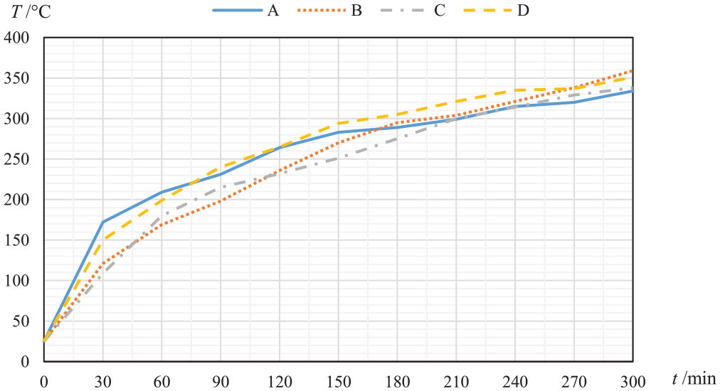
The cross-sectional areas of the circular and arc coils are 1.17 × 10⁻² m² (A₁) and 8.1 × 10⁻² m² (A₂), respectively. In addition, the number of round coil turns is 80 (n₁) and the current per turn is 180 A (I₁), the number of arc coil turns is 67 (n₂), current per turn is 80 A (I₂), cross-section coefficient is 0.95 (k). When current frequencies of the circular and arc coils are 500 and 2000 Hz, the evolutions of temperatures at points A, B, C, and D in the crankweb hole are given in Figures 18 and 19.

Figure 18.

Temperature evolution of the observation points when f = 500 Hz.

Figure 19.

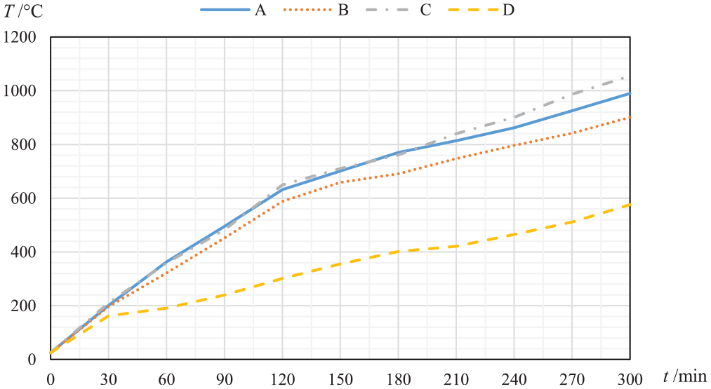
Temperature evolution of the observation points when f = 2000 Hz.

From Figures 18 and 19, it can be seen that temperature at the inner-hole surface cannot achieve the shrink-fitting requirement (320°C–370°C) after 5 h low-frequency or high-frequency heating. Also, by using low-frequency heating method for 5 h, the temperature would be stabilized, and extended heating time cannot help to meet the desired temperature.

Current density

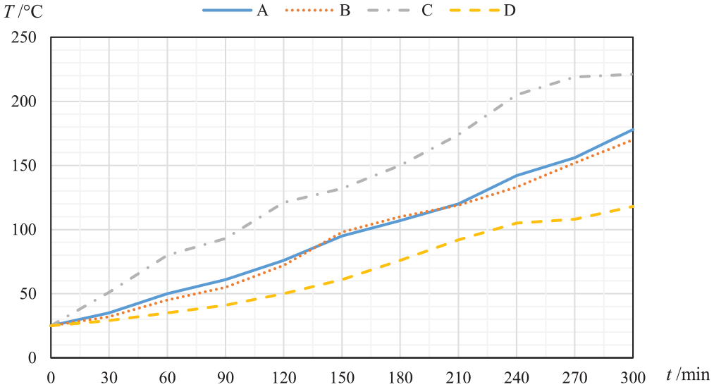
The cross-sectional areas, coefficient and current harmonic frequencies of the circular and arc coils are the same as in Section 3.3. The thickness of the coil is 30 mm. Keeping the total applied current unchanged and adjusting the thickness from 20 to 40 mm to change the current density, the current densities of the corresponding circular and arc coils are 1.85 × 10⁵, 9.92 × 10⁵, 9.23 × 10⁴, 4.96 × 10⁵ A/m². The temperature evolutions at points A, B, C, and D in the shrink-fitting hole are given in Figures 20 and 21.

Figure 20.

Temperature evolution of the observation points when δ = 20 mm.

Figure 21.

Temperature evolution of the observation points when δ = 40 mm.

It can be known from Figures 20 and 21 that when changing the current density of induction coil to 1.85 × 10⁵, 9.92 × 10⁵, 9.23 × 10⁴, and 4.96 × 10⁵ A/m², temperature cannot meet the requirements. The temperature differences among points A to D are too large, and the uniformity of the temperature distribution get worse.

Coaxiality

In actual heating process, the circular coil and the crankweb hole cannot be completely coaxial. Figures 22 and 23 present the temperature distributions at four points when the circular coil in the x and y directions deviate from the crankweb hole by 5 mm.

Figure 22.

Temperature evolution of the observation points in x direction.

Figure 23.

Temperature evolution of the observation points in y direction.

It can be seen from Figures 22 and 23 that when the original installation position of the circular coil is shifted by 5 mm along x axis, the temperature trend around the crankweb hole is almost identical after 5 h. The temperatures at points A and B are 339.42°C and 335.13°C, respectively. These two temperatures are 1.21°C and 1.13°C higher than the desired condition. Also, the temperatures at points C and D are almost unchanged. When original position of the circular coil is shifted by 5 mm along y axis, the temperature evaluations around the crankweb hole after 5 h are also basically similar. After 5 h heating, the temperatures at points C and D are 333.83°C and 342.01°C, respectively, which are 1.91°C higher and 1.06°C lower than the desired condition. Also, after 5 h, the temperatures at points A and B remained almost unchanged.

Considering the coaxiality between the circular coil and the shrink-fitting hole, the temperature variation after 5 h heating is less than 2°C when the coaxiality error is within 5 mm. The reason is that the time for heating is long enough, and the temperature of the workpiece near the coil is stabilized. The results show that the requirements for the installation accuracy of the circular coil during heating are relatively loose.

Conclusion

Compared with the original configuration with a circular coil and a rectangular coil, the modified configuration named compound circular-and-arc coil can obtain better uniform temperature distribution. This can not only reduce the warping deformation of the crankthrow, but also restrain the elliptical deformation of the shrink-fitting hole. This is conducive to improve the radial contact stress distribution, and ensure the coaxiality and parallelism between the crankthrow and the journal after shrink fitting.

Among the five factors, such as coil position, curvature, current frequency, current density, and coaxiality of the coil configuration, temperature distribution is more sensitive to the position and curvature of the arc coil. However, coaxiality nearly has no effect on the temperature distribution. Compared with the low-frequency and high-frequency heating, medium frequency induction heating leads to a better uniform temperature distribution and tend to be stable in a specified time.

Furthermore, we will (i) develop the arc-coil hardware and perform experiments to validate the effects of the modified configuration, (ii) explore the heat transfer mechanisms and the dynamic contact mechanisms in the tightening process between the crankthrow and the journal, (iii) carry out multi-physics coupling and multi-scale simulations with more comprehensive factors and more basic mechanisms, (iv) analyze the contact stress distribution and its relationship between various influencing factors, and (v) study the influence of heating temperature, assembly error / shape error, material properties, cooling air, etc. on the deformation of the assembled built-up crankshaft after shrink fitting.

Footnotes

Declaration of conflicting interests

The author(s) declared no potential conflicts of interest with respect to the research, authorship, and/or publication of this article.

Funding

The author(s) disclosed receipt of the following financial support for the research, authorship, and/or publication of this article: This research is partially supported by the National Natural Science Foundation of China (51875332), the Capacity Building Projects of Some Local Universities of Shanghai Science, and Technology Commission (18040501600).

ORCID iD

Jianguo Duan

Author biographies

Jianguo Duan received his Ph.D. degree in Mechanical Manufacturing and Automation from Tongji University, China, in 2013. He is currently a vice professor at China Institute of FTZ Supply Chain, Shanghai Maritime University, China. His main research interests include modeling and simulation of discrete manufacturing system and digital-twin driven smart manufacturing.

Qinglei Zhang received his Ph.D. degree in Mechanical Engineering from Xi’an Jiaotong University, China, in 2003. He is currently a professor at China Institute of FTZ Supply Chain, Shanghai Maritime University, China. His main research interests include digital design and manufacturing and intelligent manufacturing technology and system.

Xintao Long received his M.S. degree in Mechanical Engineering from University of Shanghai for Science and Technology, China, in 2019. He is currently an engineer at Aiways Automobile (Shanghai) Company Limited, Shanghai, China. His main research interests include finite element analysis and precise measurement and intelligent control.

Kebin Zhang received his B.S. degree in Mechatronics Engineering from Taiyuan University of Science and Technology, China, in 2007. He is currently an engineer at Shanghai Marine Crankshaft Company Limited, Shanghai, China. His main research interests include large-scale marine crankshaft manufacturing.

References

National manufacturing strategy advisory committee. China manufacturing 2025 bluebook (2018). Beijing: Publishing House of Electrics Industry, 2018. (in Chinese)

Fonte

Duarte

Anes

, et al. On the assessment of fatigue life of marine diesel engine crankshafts. Eng Fail Anal 2015; 56: 51–57.

Zucca

Mocci

. Hydrogen embrittlement and fatigue fracture of a crankshaft of an internal combustion engine. Procedia Eng 2015; 109: 202–209.

Hamrol

Ciszak

Legutko

, et al. Advances in manufacturing. Cham, Switzerland: Springer International Publishing AG, 2018.

Zhang

. Manufacturing technology development of crankshaft of marine low speed high power diesel engine in our country. Shanghai Shipbuilding 2009; 4: 38–41.(in Chinese)

Sun

, et al. Three-dimensional finite element method simulation and optimization of shrink fitting process for a large marine crankshaft. Mater Des 2010; 31(9): 4155–4164.

Kranjc

Zupanic

Miklavcic

, et al. Numerical analysis and thermographic investigation of induction heating. Int J Heat Mass Tranf 2010; 53(17–18): 3585–3591.

Lucia

Maussion

Dede

, et al. Induction heating technology and its applications: past developments, current technology, and future challenges. IEEE Trans Industr Electron 2014; 61(5): 2509–2520.

Lope

Acero

Carretero

. Analysis and optimization of the efficiency of induction heating applications with litz-wire planar and solenoidal coils. IEEE Trans Power Electron 2016; 31(7): 5089–5101.

10.

Bayerl

Duhovic

Mitschang

, et al. The heating of polymer composites by electromagnetic induction - a review. Compos Part A Appl Sci Manuf 2014; 57: 27–40.

11.

Han

Chau

Zhang

. Flexible induction heating using magnetic resonant coupling. IEEE Trans Ind Electron 2017; 64(3): 1982–1992.

12.

Sun

Qiu

. Numerical and experimental investigation of induction heating process of heavy cylinder. Appl Therm Eng 2018; 134: 341–352.

13.

Zhu

, et al. Residual stresses of polycrystalline CBN abrasive grits brazed with a high-frequency induction heating technique. Chin J Aeronaut 2019; 32(4): 1020–1029.

14.

Zhang

Zhao

Jingkuan

. Numerical simulation on induction heating process for crankshaft shrink fitting. Appl Mech Mater 2012; 215–216: 1111–1117.

15.

Cao

. Finite element method simulation of induction heating for a large marine crankshaft. Adv Mater Res 2013; 753–755: 1035–1039.

16.

Zhang

Guo

, et al. Finite element method simulation and optimization of induction heating to crankshaft shrink fitting. Chin Intern Combust Eng 2016; 37: 109–115. (in Chinese)

17.

Cho

. Coupled electro-magneto-thermal model for induction heating process of a moving billet. Int J Therm Sci 2012; 60: 195–204.

18.

Gai

, et al. Numerical simulation and experimental investigation on the induction hardening of a ball screw. Mater Des 2015; 87: 863–876.

19.

Han

Wen

. Study on electromagnetic heating process of heavy-duty sprockets with circular coils and profile coils. Appl Therm Eng 2016; 100: 861–868.

20.

Naar

Bay

. Numerical optimization for induction heat treatment processes. Appl Math Model 2013; 37(4): 2074–2085.

21.

Król

Siemiątkowski

. The analysis of shrink-fit connection – the methods of heating and the factors influencing the distribution of residual stresses. Heliyon 2019; 5(11): e02839-1–e02839-10.

Simulation study on modified coil configuration used for shrink fitting of semi-built-up crankshaft and parameters influencing the thermal distribution

Abstract

Keywords

Introduction

Configuration description

Finite element model

FEM details

Temperature distribution and thermal deformation

Influencing parameters

Position

Curvature

Current frequency

Current density

Coaxiality

Conclusion

Footnotes

Declaration of conflicting interests

Funding

ORCID iD

Author biographies

References