Locating gaps in the California Current System ocean acidification monitoring network

Abstract

Ocean acidification is a global issue with particular regional significance in the California Current System, where social, economic, and ecological impacts are already occurring. Although ocean acidification is a concern that unifies the entire West Coast region, managing for this phenomenon at a regional scale is complex and further complicated by the large scale and dynamic nature of the region. Currently, data collection relevant to ocean acidification on the West Coast is piecemeal, and cannot capture the primary sources of variability in ocean acidification through time and across the region, hindering collaboration among regional managers. We developed a tool to analyze gaps in the West Coast ocean acidification monitoring network. We describe this tool and discuss how it can enable scientists and marine managers in the California Current System to fill information gaps and better understand and thus respond to ocean acidification through the implementation of management solutions at the local level.

Introduction

In addition to contributing to climate change, anthropogenic carbon dioxide emissions have been implicated in ocean acidification (OA): “the other CO₂ problem.” ¹ When the ocean absorbs carbon dioxide from the atmosphere, the carbon dioxide reacts with water to form carbonic acid, which is further dissociated into bicarbonate and carbonate ions in a chain of equilibrium reactions that each generate a hydrogen ion (proton). The availability of bicarbonate and calcium carbonate, as either calcite or aragonite, is regulated by pH. As waters acidify with increasing partial pressure of CO₂ (pCO₂), the saturation states of calcite and aragonite decrease. ² Globally, the average ocean surface pH has declined by 0.1 unit (from 8.2 to 8.1) since pre-industrial times, representing a 26% increase in hydrogen ion concentration in seawater. ² Further increases in atmospheric CO₂ will, in turn, further increase OA; for example, surface pH is projected to decline by an additional 0.3–0.4 units under the IPCC “business as usual” scenario. ²

The West Coast of the United States is predicted to experience deleterious effects of ocean acidification (OA) sooner than many coastal regions worldwide. ³ Ocean dynamics in the region are driven by the California Current System, where upwelling brings deep, high pCO₂ water to the surface ocean, creating conditions that are naturally more acidic relative to other coastlines around the world.^3,4 In addition to anthropogenic CO₂ emissions and upwelling currents, elevated acidification in the California Current System is due to coastal erosion and runoff—all of which contribute CO₂ and nutrients to surface waters. ⁵

This OA-related decline in calcite and aragonite saturation state in coastal waters gravely threatens marine biodiversity. Aragonite is the most soluble form of calcium carbonate, and aragonite saturation state of water determines how much aragonite will dissolve in water. Many calcifying organisms produce aragonite-based shells and skeletons. Thus, organisms such as crustaceans, corals, echinoderms, mollusks, and planktonic calcifiers, like foraminifera and pteropods, respond negatively to decreases in aragonite saturation state.^6–9 These effects vary across species, but include shell dissolution, reduced growth rates, reduced fertility, or even mortality for some plankton. ⁶ While these calcifying organisms tend to be small in size and receive less conservation attention than larger fauna, they underpin many food webs in the region; a decline in marine calcifying organisms could have ripple effects on entire communities and ecosystems.^6,9,10

Beyond the ecological impacts of OA on calcifying organisms and their interrelated food webs, OA may wield significant economic impacts by placing additional pressures on fished species. OA impacts have been estimated for several important fishery species. For example, global costs of OA on the mollusk market are predicted to be more than $100 billion by 2100, assuming increasing demand and income growth. ¹¹ Regionally, larval production at oyster hatcheries on the US West Coast has suffered significant impacts due to declines in growth and survival resulting from acidified waters, ¹² threatening direct economic loss, as well as impacts to jobs. OA also threatens the cultural heritage and traditional food sources of many Native American tribes on the Pacific Coast, and impacts on shellfish affect the culture, economy, and diets of Native Americans. ¹³

The scale of this issue requires a robust contingency of stakeholders working in unity toward common efforts and integrated approaches at the ecosystem and regional scale; and to facilitate regional management of OA, scientists, federal and state policy-makers, the tribal leaders convened in 2016 to form the West Coast Ocean Acidification and Hypoxia (OAH; hypoxia, or low dissolved oxygen, is commonly found to co-occur with acidification and the two are often grouped together) Science Taskforce (“Taskforce”) as mandated by California State Assembly Bill 2139. The Taskforce worked closely with the California Ocean Protection Council to compile a monitoring inventory (OAH Inventory) with the goal of integrating OA-monitoring efforts from a multitude of research, agency, and nonprofit monitoring projects to establish a more cohesive network. A cohesive network will then enable shared learning across stakeholders, increased collaboration, and improvement of predictive models. As of April 2018, the inventory contained over 3500 records of existing datasets related to OAH, referencing data collected over the past 70 years from Mexico to Alaska.

Using this inventory to improve upon the West Coast, OA-monitoring network is a key step in improving management practices. With increased collaboration and improved understanding of spatial and temporal trends in OA, managers will be able to develop regional tactics to address the problem of OA in the California Current System more effectively. Courses of action may include but are not limited to reducing nutrient input through stakeholder involvement and updated water quality criteria, ¹⁴ implementing blue carbon techniques through submerged aquatic vegetation, ¹⁵ and on a broader scale, encouraging community reduction of greenhouse gas emissions. ¹ An improved understanding of spatial and temporal trends of OA on the West Coast, enabled by a cohesive monitoring network, will facilitate prioritization of local management solutions.

Core principles of an ideal OA-monitoring network in the California Current System have been established. ¹⁶ These principles include monitoring of aragonite saturation state, collecting data at a temporal frequency that captures changes in aragonite saturation state, and ensuring public access to data. However, historic and current monitoring sites were established for specific research or management objectives and not with the goal of creating a regional monitoring network. Given the current state of West Coast OA monitoring, not all monitoring efforts provide the same level of quality control or data relevant to management needs. Data collection varies in the equipment used, the parameters measured, and the frequency of data collection. In situ sensors, moorings, and buoys can give temporally resolved data, also with varying levels of precision, but give little information on spatial patterns. These types of monitoring are common along the coast, where they can be more easily accessed for service, repair, and collection. Gliders and cruises can cover great distances and give more information on spatial patterns, particularly offshore, but are difficult to repeat and thus do not give information on temporal trends. Acidification can be measured in many different ways, depending on the questions being asked and the ecosystem response being evaluated. It is commonly measured with pH, with records on the West Coast beginning as early as 1949. ¹⁷ However, pH does not have the same direct implications on biology that aragonite saturation state does. For this reason, aragonite saturation has been identified as the ideal metric of OA in the California Current System, ¹⁶ though it is more expensive and difficult to derive because it requires making a calculation using measurements of two carbonate parameters as opposed to just measuring one, as is the case with pH. Other common parameters measured include pCO₂ of surface water, pCO₂ of air, dissolved inorganic carbon (DIC), and total alkalinity (TA). Each of these parameters measures one part of the carbonate system, but alone does not yield information on the saturation state of aragonite. Another great challenge in monitoring and managing OA is that species often respond to short-term, acute OA events, yet monitoring is rarely able to capture these due to insufficient spatial and temporal resolution.

High frequency measurements that enable calculation of aragonite saturation state are spatially sparse and so a meaningful interpolation of typical conditions is impossible. Observations that have adequate spatial coverage are from cruises, and can thus create a snapshot in time of aragonite saturation state. These types of cruise data have been used to determine aragonite saturation state in the California Current System during a narrow time frame, ¹⁸ but acidification conditions depend strongly on seasonal cycles, and so such a snapshot does not necessarily capture typical conditions. Due to this lack of spatially and temporally resolved carbonate system data and the trade-off between temporal and spatial resolution, high-resolution modeling of the carbonate system has become an active area of research.^19,20 However, the development of physics-based models relies on evaluation of model performance, which in turn requires observational data. Thus, whether using observational data or model outputs to understand acidification conditions in the California Current System, high quality, highly resolved data are required.

The purpose of our study is to quantify monitoring gaps in an OA-monitoring network and then use that framework to identify locations within the US West Coast region (California, Oregon, and Washington) where existing monitoring efforts are inadequate to characterize aragonite saturation state. We also conducted focused analyses to characterize the different types of monitoring gaps in the West Coast region (aragonite saturation data gaps and high-frequency monitoring gaps) to help managers meet the goals of the Taskforce. This analysis is based on the existing monitoring network, but could be applied to any given network of monitoring assets to fill gaps, and could be used iteratively as an optimization tool to design a new network.

This work builds on a wide and varied history of analyzing gaps in monitoring networks. These analyses have been done in the fields of water and air quality, meteorology, and oceanography, among others.^21–24 For example, marine-monitoring networks have been analyzed to find gaps in marine-life monitoring, ²⁵ in monitoring of habitat types, ²⁶ and in a monitoring network for harmful algal blooms. ²⁷ All of these studies employed different methods depending on the goal and the data available. One study uses satellite data to determine cross-shore decorrelation scales and in situ moorings to quantify temporal decorrelation at five different locations on the coast, and quantifies the performance of a sparse monitoring network based on the resulting covariance matrix. ²⁷ Other studies use metadata of existing monitoring (i.e. type of information collected and location) to analyze data gaps based purely on regional distribution of and geographic distance to monitoring.^25,26

We developed methods taking into consideration what has already been done and how our data and goals fit into the existing body of literature: similar to the study by Frolov et al., ²⁷ we are searching for gaps in a network that measures a chemically and biologically driven phenomenon in the ocean (the balance between primary production and respiration is a strong control on ocean acidity); similar to the study by Asch and Turgeon ²⁶ and Kot et al., ²⁵ our analysis finds gaps in an extensive network, and relies on metadata of the network as opposed to data collected at each monitoring site. Thus, our analysis seeks an approach that falls within this spectrum: with a lack of highly resolved spatial data, and with limited access to time-series data, how can we improve on the existing, but non-cohesive OA-monitoring network while considering oceanographic conditions across the region?

Methods

Overview

Our analysis locates the best site for the next monitoring asset given the existing monitoring network, thereby filling in monitoring network gaps one asset at a time, based on the sites that already are in place. In this analysis, we utilized methods that fall in the middle of the spectrum defined by other works in this realm (see study by Asch and Turgeon ²⁶ for a more simplistic approach, and study by Frolov et al. ²⁷ for a more involved approach). These decisions were made due to the constraints of the data we used (spatial metadata as opposed to time-series and satellite data) as well as the goal of working with policymakers and non-scientist end users. The result is an analysis that provides specific spatial information on relative sampling of OA on the West Coast.

Monitoring networks are geographic objects, and it might seem that the ideal network would be evenly spaced across the ocean. However, the ocean is not uniform: some places in the ocean are more dynamic than others, with change driven by both vertical and horizontal movement of properties on short timescales. This effect can be illustrated with an example from the Santa Barbara Channel. A correlation matrix of aragonite saturation state time-series data in the Santa Barbara Coastal Long Term Ecological Research Project (SBC LTER) (Table 1) reveals correlations between locations that are disproportional to distances between locations; a negative correlation exists between Mohawk Reef ²⁸ and Santa Barbara Harbor, ²⁹ which are less than 5 km apart, while the strongest correlation is between Alegria ³⁰ and Arroyo Quemado Reefs, ³¹ which are 16 km apart (Table 1). This example shows quantitatively that considering geographic distance alone will not optimize a monitoring network, especially at a large regional scale.

Table 1.

A correlation matrix of aragonite saturation state time series data from the SBC LTER: Alegria Reef (−120.28998, 34.46085), Arroyo Quemado (−120.11965, 34.46495), Mohawk Reef (−119.73012, 34.39323), and Santa Barbara Harbor (−119.68493, 34.40934).

	Alegria Reef	Arroyo Quemado Reef	Mohawk Reef	Santa Barbara Harbor
Alegria Reef	1.00	16	52	56
Arroyo Quemado Reef	0.39	1.00	37	40
Mohawk Reef	0.11	0.14	1.00	5
Santa Barbara Harbor	0.03	0.33	−0.07	1.00

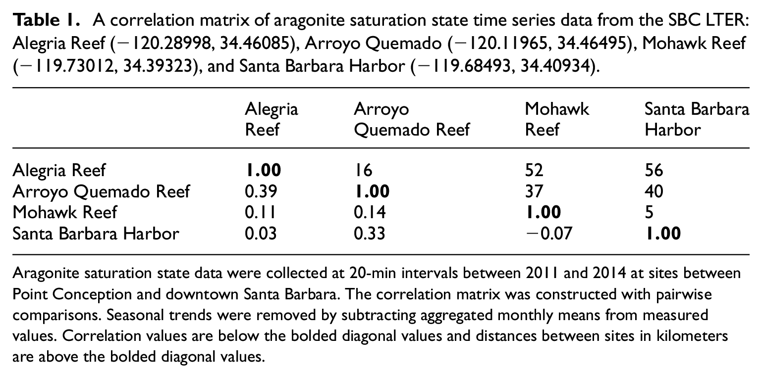
Aragonite saturation state data were collected at 20-min intervals between 2011 and 2014 at sites between Point Conception and downtown Santa Barbara. The correlation matrix was constructed with pairwise comparisons. Seasonal trends were removed by subtracting aggregated monthly means from measured values. Correlation values are below the bolded diagonal values and distances between sites in kilometers are above the bolded diagonal values.

Thus, where the ocean is highly dynamic, an ideal monitoring network will have more closely clustered assets than in places that are more static. ³² Consideration of variance is common in oceanography, ²⁷ but has not been considered in all previous marine-monitoring network gap analyses.^25,26 In the absence of highly resolved time series and spatial data that are representative of our study region, we developed a method to gain a relative index of spatial variance in order to take horizontal oceanographic heterogeneity into consideration within the mixed layer. To achieve this, we combined the spatial variance of estimated aragonite saturation state with geographic distance, and used this metric to recommend locations for additional or enhanced monitoring. The code and all publicly accessible datasets used in this project are freely available online at resilienseas.github.io.

Existing monitoring network

Our primary data source was the West Coast OAH Monitoring Inventory (downloaded on 22 February 2018), a dataset containing metadata about each monitoring asset. Monitoring assets include survey areas, cruise stations, gliders, sample sites, shore-side sensors, and moorings. The dataset includes information describing the OA parameters collected, the frequency and duration of collection, and the monitoring locations. OA parameters collected include pCO₂ of surface water, pCO₂ of air, pH, DIC, TA, carbonate ion, and dissolved oxygen. While we had access to the inventory containing metadata on West Coast oceanographic monitoring, we did not have access to all the data collected at each monitoring asset, because assets varied in the degree of open access. Some assets included in the inventory produce publicly available data; some release recent observations while keeping long-term records private, and data from some existing assets are only available in aggregate upon request at the discretion of the contributor. These varying levels of privacy are due to the goals of the organization collecting data. For example, the monitoring inventory includes data collected by scientific researchers, some of which are publicly available, some of which are available by request, and some of which are embargoed until a future publication; the monitoring inventory also includes data collected by shellfish hatcheries, which tend to have excellent time series of aragonite saturation state, but may consider water quality data proprietary, and thus may not make the data public except upon request and at their own discretion. We included all assets in the inventory in this analysis, regardless of privacy standards. The assets that do produce publicly available long-term records of aragonite saturation state are mostly in the SBC LTER Project, and are thus not representative of the entire coast. We used the metadata to determine whether or not each asset was “carbonate complete,” meaning the asset collects parameters needed to determine aragonite saturation state (at least two of pH, TA, DIC, and pCO₂).

Estimating aragonite saturation state

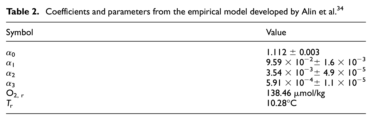
We based our analysis on the metric of aragonite saturation state, which has been identified as a gold standard of an ideal OA-monitoring network. ¹⁶ The variables needed to calculate aragonite saturation state are not yet measured at a sufficient spatio-temporal resolution to identify highly variable locations across the study region. We used temperature (T) and dissolved oxygen (O₂) as proxies, because they are strongly positively correlated with aragonite saturation state.^33,34 At a subregional scale, empirically derived linear models predict aragonite saturation state based on temperature and dissolved oxygen measurements.^33,34 Alin et al. ³⁴ developed an empirical relationship to predict aragonite saturation state in the southern California Current System (defined as the region between Monterey Bay, CA and Punta Eugenia, Mexico), with a final R ² value of 0.988 (see Table 2), and Juranek et al. ³³ developed a similar relationship to predict aragonite saturation state in the Pacific Northwest (defined as the Oregon Coast and the outer coast of Washington), with a final R ² value of 0.987 (see Table 3).

Table 2.

Coefficients and parameters from the empirical model developed by Alin et al. ³⁴

Symbol	Value
α 0	1.112 ± 0.003
α 1	9.59 × 10−2± 1.6 × 10−3
α 2	3.54 × 10−3± 4.9 × 10−5
α 3	5.91 × 10−4± 1.1 × 10−5
O2, r	138.46 μmol/kg
T r	10.28°C

Table 3.

Coefficients and parameters from the empirical model developed by Juranek et al. ³³

Symbol	Value
α 0	9.242 × 10−1± 4.4 × 10−3
α 1	4.492 × 10−3± 5.0 × 10−5
α 2	9.40 × 10−4± 3.4 × 10−5
O2, r	140 μmol/kg
T r	8°C

Our analysis utilized equation (2) from Alin et al. ³⁴ in the southern part of our study region

$${\mathrm{\Omega }}_{\mathrm{arag}}={\alpha }_0+{\alpha }_1({\mathrm{O}}_2-{\mathrm{O}}_{2,\mathrm{r}})+{\alpha }_2(T-T_{\mathrm{r}})+{\alpha }_3(T-T_{\mathrm{r}})\times ({\mathrm{O}}_2-{\mathrm{O}}_{2,\mathrm{r}})$$

(1)

and equation (3) from Juranek et al. ³³ in the northern part of the study region

$${\mathrm{\Omega }}_{\mathrm{arag}}={\alpha }_0+{\alpha }_1({\mathrm{O}}_2-{\mathrm{O}}_{2,\mathrm{r}})+{\alpha }_2(T-T_{\mathrm{r}})\times ({\mathrm{O}}_2-{\mathrm{O}}_{2,\mathrm{r}})$$

(2)

In both empirical relationships, T_r and O_2r are reference values for temperature and dissolved oxygen, respectively.

We extracted sea surface temperature and in situ dissolved oxygen data from the Bio-ORACLE global dataset. ³⁵ Since its initial publication in 2012, Bio-ORACLE data have been utilized extensively in published literature. ³⁶ All parameters are available at a 9.2 km² resolution. Mean sea surface temperature in Bio-ORACLE is derived from monthly Aqua-MODIS climatologies from 2002 to 2009. ³⁷ Mean dissolved oxygen in Bio-ORACLE is derived from 5,40,582 in situ measurements from the 2009 World Ocean Database. ³⁸ The Bio-ORACLE dissolved oxygen layer was created from a data interpolating variational analysis, a method which has been used previously in oceanographic records.^39–41

Both Juranek et al. ³³ and Alin et al. ³⁴ note that their models should be used with in situ measurements, below 30 m and 15 m depth, respectively, of dissolved oxygen and temperature as opposed to sea surface measurements, in order to be removed from atmospheric influence. The dissolved oxygen data from Bio-ORACLE are in situ measurements, but the sea surface temperature data are remotely sensed at the surface of the ocean. To account for differences between temperature measured at the sea surface and below the mixed layer, we subtracted 0.7°C from sea surface temperature, which is in the range of commonly used differences between temperature at the surface and below the mixed layer, ⁴² and was chosen to achieve greatest agreement with observational data. ³⁴

Temperature and oxygen data were loaded into R (version 3.4.3) ⁴³ using the “smdpredictors” package, ⁴⁴ projected to North American Datum 83 California Teale Albers, and cropped to our study region, identified by the bounding box of NAD 83 coordinates (−50000, 340000, −600000, 1210000). Because both the Juranek et al. ³³ and Alin et al. ³⁴ empirical relationships were developed for the coastal ocean and have not been validated for estuarine regions where other sources of DIC and TA may cause the linear relationships to change due to freshwater and industrial sources of carbon, we removed Puget Sound and San Francisco Bay from our analysis.

We then created an aragonite saturation state raster following equation (1) for the southern region and equation (2) for the northern region, using the mean sea surface temperature and mean dissolved oxygen values from each ocean area. In other words, the Alin model was used to predict aragonite saturation state from waters off the southern border to waters off Davenport, CA, and the Juranek model was used to predict aragonite saturation state from waters off the northern border to waters off the California and Oregon border. To reduce the effect of the abrupt change in aragonite saturation state at the boundary between the two models, the mean of the two model outputs was used to predict aragonite saturation state in waters between the Point Mendocino, CA and Point Arena, CA. The mean of both models and the Juranek model were averaged between Point Mendocino, CA and Point St George, CA. The mean of both models and the Alin model were averaged between Point Arena, CA and Point Montara, CA.

This depiction of aragonite saturation state (Figure 1) is consistent with other work,^20,45 with strongest acidification and upwelling conditions between Point Conception, CA and Cape Blanco, OR, with a peak between Point Arena, CA and Cape Mendocino, CA. We calculated a mean estimate of aragonite saturation state across all California Cooperative Oceanic Fisheries Investigations (CalCOFI) cruise stations of 2.245, which is consistent with the mean aragonite saturation state estimated by Alin et al. ³⁴ from temperature and dissolved oxygen measurements from CalCOFI cruise stations from 2005 to 2011 at 20 m depth (0.13% relative error). Our findings were also consistent with calculated aragonite saturation state from carbonate parameters from CalCOFI cruises by Alin et al. ³⁴ We utilized this relative error to account for uncertainty.

Figure 1.

Aragonite saturation state in the study region as predicted by equations from Alin et al. ³⁴ and Juranek et al., ³³ using mean sea surface temperature of monthly climatologies from 2002 to 2009 derived from AQUAMODIS, and dissolved oxygen data from the 2009 World Ocean Database, both obtained through Bio-ORACLE. Sea surface temperature was corrected by −0.7° to account for the temperature difference between the surface and the base of the mixed layer. ⁴² Aragonite saturation state in the transition region from the California–Oregon border to Davenport, CA was determined by the combinations of the two empirical models.

Utilizing the monitoring inventory

We used Voronoi polygons to divide the ocean into regions based on spatial proximity to each monitoring asset, and to compare temperature and dissolved oxygen at monitoring assets to the surrounding ocean conditions. ⁴⁶ This methodology requires a set of points, and yields a set of polygons, each of which is centered around a single point. Each polygon encompasses all the space that is closer to the point within the shape than to any other point provided. Voronoi polygons are thus a simple and useful way to divide our study region by proximity to each monitoring asset. We assigned a polygon identification number to each polygon and then gridded the Voronoi polygons, while maintaining the polygon identification numbers. We assigned the aragonite saturation state value of all points with the same polygon identification number to the estimated aragonite saturation state value of the cell containing the monitoring asset associated with that same polygon identification number. This step resulted in a map of aragonite saturation state across the West Coast estimated by the Juranek and Alin empirical linear model outputs at each monitoring site. Thus, a monitoring network with 20 assets would result in a map made up of 20 parcels of area, each with different values of aragonite saturation state based on the estimated value at the nearest monitoring asset.

We then used the empirical model outputs created using the continuous layers of temperature and dissolved oxygen to find the difference between the empirical model outputs at every location in the ocean and the empirical model outputs for the nearest monitoring asset. In this calculation, we included uncertainty at both locations, that is, if the aragonite saturation state is greater at a given location than it is at the nearest monitoring site, we accounted for negative error in the first term and positive error in the second term, and vice versa. The result is an aragonite saturation state discrepancy value that describes differences in the acidification conditions at any point on the West Coast as compared to these conditions at the nearest data collection locations. In places where this value is high, a monitoring asset is not describing OA conditions well. In places where this value is low, a monitoring asset describes OA conditions very well.

To quantify this relationship between changing aragonite saturation state and distance, the aragonite saturation state raster was used to create a semi-variogram. ⁴⁷ The semi-variogram describes the expected value of the semi-variance ${(x_k-x_l)}^2/2$ , which is half the squared discrepancy, as a function of the distance between points l and k. This relationship expresses how the semi-variance of a parameter increases with distance, revealing information on the spatial scale of decorrelation of that parameter. In this analysis, we used it to determine the relationship between variance in aragonite saturation state and distance. The semi-variogram revealed that the semi-variance in aragonite saturation state does not saturate (i.e. the semi-variance increases continuously as distance increases), and that a linear relationship describes this relationship (P << 0.05 and R² = 0.995)

$$\mathrm{semivariance}=(4.472\times {10}^{-8})\times \mathrm{distance}.$$

(3)

The inverse of equation (3) was used to define “oceanographic distance”

$$\mathrm{oceanographic}\mathrm{distance}=\left(\frac{\frac{{(x_k-x_l)}^2}{2}}{4.472\times {10}^{-8}}\right),$$

(4)

where x_k and x_l are the estimated aragonite saturations at locations k and l. For each cell k, we set l as the location of the nearest monitoring asset and used equation (4) to calculate the oceanographic distance to that asset (Figure 2). This oceanographic distance is a theoretical construct and is calculated to be able to combine geographic distance and aragonite saturation discrepancy in one expression, in order to determine the “effective distance” between two points in kilometers.

Figure 2.

Oceanographic distance to nearest monitoring in kilometers. Red regions have acidifications that are different from conditions at the nearest monitoring asset, and thus are effectively distant, and blue regions have acidification conditions that are similar to conditions at the nearest monitoring asset, and thus are effectively close. Black dots represent monitoring assets in the inventory where ocean acidification relevant information is being collected.

Quantifying gaps

We used a Euclidean distance approach to combine geographic distance and oceanographic distance into a single “gap” layer. Thus, a gap in the network is a place where oceanographic conditions are different from conditions at the nearest data collection location, a place that is geographically far from the nearest data collection, or a place with both of these characteristics. When combining these two, we weighted the oceanographic distance term by multiplying it by the unitless ratio of the maximum value of geographic distance (210 km) and the maximum value of the oceanographic distance (489 km). This was done to account for differences in scale between geographic distance and oceanographic distance, such that the effective distance to nearest monitoring weights the two equally, rather than weighting oceanographic distance more. The result describes the effective distance to the nearest monitoring asset in kilometers, based on geographic distance and oceanographic conditions. Equation (5) describes the equation we developed to describe gaps in OA-monitoring efforts

$$\begin{array}{c}\mathrm{Effective}\mathrm{distance}\mathrm{to}\mathrm{nearest}\mathrm{monitoring}=\hfill \\ \sqrt{{(\mathrm{geographic}\mathrm{distance})}^2+{(\frac{\mathrm{maximum}\mathrm{geographic}\mathrm{distance}}{\mathrm{maximum}\mathrm{oceanographic}\mathrm{distance}}\times \mathrm{oceanographic}\mathrm{distance})}^2}\hfill \end{array}$$

(5)

We repeated this analysis with subsets of the inventory to examine different types of gaps, such as carbonate complete monitoring and high-frequency monitoring (monitoring that collects data at least once per day). These focused gap analyses describe two crucial elements of an ideal OA-monitoring network: direct measurements of aragonite saturation state and a sufficient frequency to capture the scale of temporal variation in acidification. ¹⁶ We examined the highest-frequency OA data available, collected by the Santa Barbara Channel LTER project, to understand the nature of temporal variability of aragonite saturation state, and we found temporal decorrelation scales with a 1/e significance level ²⁷ (i.e. the time at which correlation reaches a level of 1/e, or 0.367) ranging between 1.2 and 1.4 days after seasonal variation in aragonite saturation state was removed (Figure 3) . Thus, we defined “high frequency” as monitoring that occurs at least daily, in order to capture temporal decorrelation scales of aragonite saturation state. To generate the carbonate complete gap analysis, we filtered the inventory to only analyze assets that collect data for at least two carbonate complete parameters (the minimum necessary to calculate aragonite saturation state).

Figure 3.

Temporal decorrelation scales with a 1/e significance level for aragonite saturation state measurements in the Santa Barbara Channel LTER, corrected for seasonal variability. The thick black line signifies the 1/e significance level. The sites are spread across a distance of 65 km between the Gaviota Coast and the Santa Barbara Harbor. Correlation, shown by the colored lines, drops below 1/e, or 0.367, just after 1 day at all four sites, suggesting decorrelation timescales are tightly clustered between 1.2 and 1.4 days.

Results

Gaps in the full inventory

With an estimate of average acidification conditions across the whole region, we can locate monitoring gaps based on the entire inventory, including both past and present monitoring efforts, to assess where future monitoring efforts should be focused. The results of the gap analysis (Figure 4) revealed that the largest gaps in the West Coast OA-monitoring network are offshore from Cape Blanco, OR, at the mouth of San Francisco Bay, and at Dana Point, CA. Washington has greatest coverage.

Figure 4.

Gaps in ocean acidification monitoring on the West Coast. Units represent the effective distance (a combination of oceanographic distance and geographic distance) to the nearest monitoring asset in kilometers. Black dots represent existing monitoring sites. Gaps exist at Dana Point CA, at the mouth of San Francisco Bay, and offshore from Cape Blanco, OR, as well as offshore from cruise stations.

Carbonate complete gaps

We analyzed gaps in the subset of the West Coast monitoring inventory that collects two or more carbonate parameters, allowing the aragonite saturation state to be calculated (Figure 5). The greatest gap is offshore from Santa Cruz, CA. Additional gaps exist at Dana Point, CA and offshore from Cape Blanco, CA.

Figure 5.

Gaps in carbonate complete ocean acidification monitoring on the West Coast. Units represent the effective distance (a combination of oceanographic distance and geographic distance) to the nearest monitoring asset in kilometers. Black dots represent monitoring assets that currently are carbonate incomplete and are part of ongoing monitoring projects, and thus could be modified to collect two carbonate measurements. Gaps exist at Santa Cruz, CA; Dana Point, CA; and offshore from Cape Blanco, OR.

High-frequency gaps

We also analyzed gaps in the subset of the inventory that collects OA-relevant data at least once per day (Figure 6). Results reveal nearshore gaps at Cape Meares, OR, and the mouth of San Francisco Bay, with less severe gaps on the Bug Sur Coast and at the California–Oregon border. Results also highlight that certain high frequency monitoring assets are currently playing key roles in providing high-frequency OA data. Specifically, the CCE01 and CCE02 moorings in Central California, the OASIS Moorings in Monterey Bay, and the cabled and wire following moorings in Oregon and Washington, are playing key roles in providing high frequency offshore time series.

Figure 6.

Gaps in daily ocean acidification monitoring on the West Coast. Units represent the effective distance (a combination of oceanographic distance and geographic distance) to the nearest monitoring asset in kilometers. Black dots represent monitoring assets that are currently collecting data daily. Onshore gaps exist at Cape Meares, OR, the mouth of the San Francisco Bay, on the Big Sur Coast, and at the California–Oregon border. Offshore gaps are pervasive throughout the region.

Discussion

OA in the California Current System is a seemingly intractable issue that unites stakeholders across a variety of ecosystems along the West Coast. Though the root cause of this problem is much larger than the scale of the California Current System itself, regional actions may help to mitigate or ameliorate the effects of OA. We provide the first known description of OA-monitoring assets and gaps off the West Coast. Based on this analysis, we highlight monitoring gaps at the mouth of San Francisco Bay, at Dana Point, CA and offshore from Cape Blanco, OR.

The data gap at the mouth of the San Francisco Bay is likely due to the gradient between ocean and estuarine conditions that occurs at the Golden Gate. The nearest monitoring to this data gap is in Richardson Bay, which, as an estuarine site, may not represent this region well. The nearest ocean monitoring to this region are the Rockfish Recruitment and Ecosystem Surveys, which are cruise stations 25 km off the coast, and likely do not capture the tidal influence of the bay and delta. This data gap could be filled by shore-side data collection offshore from Ocean Beach in San Francisco or Muir Beach in Marin. We suspect the gap at Dana Point is due to complex oceanography and shadowing caused by the Channel Islands, as suggested by Figure 1. In addition, the Southern California Bight Regional Monitoring Program through the Southern California Coastal Water Research Project currently monitors the region with closely spaced cruise lines throughout the Bight, which are supplemented by the NOAA OA cruises and CalCOFI cruises; however, between these three organizations, there is no monitoring between Oceanside, CA and north of Dana Point, CA. This gap is clear in Figure 4. We suggest emphasizing this region in future cruise programs. Finally, we suspect the monitoring gap offshore from Cape Blanco is due to geographic distance to monitoring in the region. The closest cruise line to the south runs off the coast from the California–Oregon border, and the closest cruise line to the north runs offshore from Coos Bay, creating a distance of over 170 km between offshore measurements; this is the greatest distance between cruise lines throughout the region. We suggest that future cruises focus on collecting data in this region.

The carbonate complete monitoring gaps identified in Figure 5 could be filled by adding an additional sensor to existing monitoring infrastructure that currently only collects one carbonate parameter. Specifically, CalCOFI cruises could strategically collect carbonate complete measurements on either side of the Dana Point data gap; the CenCOOS shore-side sensor in Santa Cruz could collect carbonate complete measurements to fill the carbonate complete data gap in that region, and NOAA fish recruitment and survival surveys in Northern California and Oregon could strategically collect carbonate complete measurements to address data gaps in those regions.

The results of the high-frequency gap analysis, shown in Figure 6, illuminate the importance of existing daily monitoring, particularly the CCE1 and CCE2 moorings operated by Scripps, the OASIS moorings maintained by the Monterey Bay Aquarium Research Institute, and the cabled and wire-following moorings offshore from Washington and Oregon and operated by a suite of organizations including Oregon State University, The Ocean Observatories Initiative, NOAA Pacific and Marine Environmental Laboratory, and the Oregon Department of Fish and Wildlife. The near-shore regions identified in Figure 6, including Cape Meares, OR, the California–Oregon border, the mouth of the San Francisco Bay, and the Big Sur Coast should be prioritized in future expansion of the high-frequency monitoring network.

This tool can be updated with improved data inputs for the West Coast in the future, or adapted for use in other ocean regions. As the West Coast OA-monitoring network is grown and existing gaps are filled, this analysis can be repeated. We have explicitly discussed steps to fill the most extreme data gaps identified in this analysis, but this analysis reveals a gradient of data gaps across the coast. Thus, as the monitoring network is improved and expanded upon, lower-severity data gaps can be filled in a triage approach, filling the less extreme gaps once the most extreme gaps have been filled. All of the code used to conduct these analyses is freely available online at resilienseas.github.io, and will yield reproducible results with any given set of monitoring assets and corresponding spatial extent. Open science is vital for these types of management-relevant questions, and we made our entire analysis available in an effort to meet the goal of publicly available OA data in an ideal monitoring network, ¹⁶ and more broadly as a contribution to the open science community.

Management

Results from the gap analysis reveal several possible management actions that can be taken to fill priority areas for additional monitoring. Because we designed our methods to identify the highest-value single additional monitoring gap to fill, even incremental additions of a few sensors or new sampling sites will greatly improve the West Coast OA-monitoring landscape. The priority areas for additional monitoring infrastructure are at Dana Point, CA at the Golden Gate, and offshore from Cape Blanco Oregon. We recommend that any additional monitoring in that region should collect data at a daily frequency or greater, and should collect carbonate complete data. High-frequency data collection in this region will provide information on short-term changes, such as within diurnal or tidal cycles, as well as changes in response to short-lived upwelling events, ¹⁶ and maintaining existing offshore high-frequency monitoring should be a high priority. By adding additional instrumentation to existing infrastructure at monitoring sites identified in Figure 5, existing monitoring can become carbonate complete monitoring. Measuring any component of the carbonate system is useful—measuring just pH or just pCO₂ gives important insight into stressors and habitat quality for marine organisms, and there are strong linkages between pH and pCO₂ and metrics such as growth rate and shell thickness. ⁴⁸ Aragonite saturation state is the most direct link between acidification condition and biological response, and defining aragonite saturation state constrains the entirety of the inorganic carbon system, allowing inferences of numerous parameters that can be used to evaluate biological effects of changing ocean chemistry. Without aragonite measurements, the rest of this information is lost—thus, an ideal monitoring network will contain carbonate complete monitoring assets to allow users to calculate aragonite saturation state from the data collected at each asset.

Furthermore, though research shows that marine ecosystem exposure to OA follows latitudinal gradients on the West Coast with greater exposure in higher latitudes, these estimates are based on annual mean of surface aragonite saturation state values. ⁵ While annual means are a useful metric for long-term trends, a primary driver of OA on the West Coast is episodic upwelling, which can lower surface aragonite saturation state drastically for a short time. Regional Oceanographic Modeling System (ROMS) analyses show that coastal upwelling on the West Coast peaks between Cape Blanco in Oregon and the Channel Islands in Southern California. ⁴⁵ Thus, despite latitudinal gradients in mean annual exposure, short-term exposure not captured in annual mean measurements is likely across a large section of the southern half of our study region. Experiments at shellfish hatcheries show that a decrease in aragonite saturation state of waters in which shellfish were spawned and reared for the first 48 hours of life is correlated with reduction in both larval production and mid-stage growth, ⁴⁹ suggesting that decreases in aragonite saturation state on the timescale of upwelling events (weeks) can have deleterious effects on marine species. Thus, capturing short-term variability driven by upwelling is essential, making it necessary to monitor for OA across our study region and at high temporal frequencies, despite latitudinal gradients in annual mean values of surface aragonite saturation state.

Establishing a more cohesive network by integrating these OA-monitoring efforts from a multitude of research, agency, and nonprofit monitoring projects will enable more accurate predictive abilities as well as more effective development and implementation of regional management. As monitoring networks and OA prediction improves, it is important that these data are used to inform policy. Further, marine managers can be more effective in their management strategies when scientists and data collectors host data publicly. With improved information about the level of OA threat now and into the future, marine managers will be able to pursue local mitigation efforts to increase ecosystem resilience to OA. Here, we discuss several management actions that can be taken to decrease OA threat locally.

1. Minimize the input of local water pollutants, such as nitrogen, phosphorus, and organic carbon into coastal watersheds: Nutrients in the form of nitrate and phosphate can lead to eutrophication of near-shore coastal waters, creating hypoxic conditions, which often coincide with high seawater pCO₂ and increased acidity. ¹⁴ Thus, by reducing the drivers of localized hypoxic events, communities can also minimize exacerbations to OA.

2. Update water quality criteria to address OA: The standards for pH have remained unchanged since the Clean Water Act was written, ⁵⁰ and could be fine-tuned to a narrower range based on biological thresholds. This could increase the amount of coastal waters listed as “impaired” on the Clean Water Act 303(d) list, ⁵⁰ which would raise awareness of acidic conditions to managers and local decision-makers while opening up sources of funding to ameliorate OA stress. However, there are substantial hurdles to changing water quality criteria, namely funding and an arduous bureaucratic process.

3. Utilize aquatic vegetation as a tool for decreasing CO₂ in local waters: The basis of this method is to protect habitats that sustain ecological and biogeochemical functions. Thus, existing aquatic vegetation can be protected, specifically in places where it may ameliorate local pH through carbon sequestration into marine sediments. ¹⁵ This strategy addresses the ecological and biological concerns of OA. Conservation of submerged aquatic vegetation will be important for maintaining naturally occurring OA mitigation. Furthermore, finding suitable areas for the restoration of submerged aquatic vegetation will benefit OA vulnerable species and communities.

Ultimately, the scale of this issue requires a robust contingency of stakeholders working in unity toward common efforts and integrated approaches at the ecosystem and regional scale. Local management actions, however, are an excellent starting point. By improving the existing monitoring network, we can improve our understanding of OA in space and time, better detect future changes due to increased atmospheric CO ² , and begin prioritizing when and where local management solutions can most effectively reduce the threat of OA. Successful data-driven management requires effective monitoring and predictive capabilities. The results of this study present a pathway forward to meeting these goals.

Future applications

To address specific management interests, this analysis could be modified to prioritize monitoring in specific management zones or habitat for economically important species. For example, if stakeholders in the West Coast Dungeness crab fishery were interested in improving OA monitoring as it relates to the health of the fishery, prioritization could be placed on monitoring within Dungeness crab habitat by weighting final the effective distance more heavily within the habitat (e.g. with a multiplier), resulting in a gap analysis of the study region that prioritizes filling gaps within Dungeness crab habitat. This same approach could be used by management groups across the coast, including National Marine Sanctuaries, National Parks, marine reserves, and NOAA-designated essential fish habitat. Managers and scientists have indicated the importance of having monitoring in and outside of these managed areas, ⁵¹ emphasizing the need for collaboration and cooperation across management organizations.

In addition, since the goal of an improved OA-monitoring network is ultimately to better predict deleterious effects of OA on marine organisms, long-term biological monitoring paired with long-term aragonite saturation state monitoring is necessary, as this combination yields information both on the level of threat, as well as the biological response. ¹⁶ While changing ocean chemistry impacts ocean biology, changing ocean biology, in turn, impacts ocean chemistry. ⁵² Interactions between ocean chemistry and biology are complex and interactive, and adaptive capacity of marine species to changing carbonate chemistry is an active field of research.^48,53 This type of research is crucial to furthering the scientific understanding of spatio-temporal trends in aragonite saturation state, biological responses to these changes, and feedbacks between chemistry and biology. Pairing of physical and biological monitoring is essential to understanding these links and thus in the future, this analysis could be repeated with paired biological monitoring to improve regional understanding of these interactions.

Finally, it is important to note that the solution this tool currently provides is a greedy heuristic. With a given set of existing monitoring assets, the analysis reveals the best place to put the next monitoring asset. The result is designed to inform the selection of additional sites for monitoring, not the wholesale design of an optimal coast-wide monitoring network. However, our method of quantifying gaps in OA monitoring can be adapted to design a monitoring network from the ground up. This could be done by setting an initial number of monitoring points and using our framework to analyze the gaps in the randomly designed network. To optimize the network, this would be repeated iteratively, similarly to the process MARXAN uses when designing reserve networks, ⁵⁴ though in this case, the objective function would be the integrated gap value of the entire study region. Thus, after generating a given number of random monitoring network designs—MARXAN guidance documents recommend using a minimum of 100,000 iterations ⁵⁴ —the design with the optimum overall coverage would be selected. Similarly, if the user wanted to preserve certain monitoring sites that had external reasons to be there (for example, monitoring at shellfish hatcheries or long-term ecological research sites), these chosen locations could be used along with any number of other random sites, and the same process carried out. The end result would be a monitoring network that contained the preserved sites, with an optimal network designed around them. This would be a novel and powerful way to approach OA-monitoring network design in the ocean.

Limitations

Since empirical relationships for estimating aragonite saturation state from temperature and dissolved oxygen have not been developed for estuarine regions, we were not able to include these regions in our analysis. This is a significant limitation, because estuarine environments are often subject to industrial sources of nutrients and carbon, and aragonite saturation state in these places is often very low. ⁵⁵ Monitoring of these trends in estuaries is essential, and we recommend that this analysis be repeated at a point in the future when empirical relationships to estimate aragonite saturation state in estuaries exist.

The existing monitoring inventory does not include information about the depths of data collection. Seawater in the California Current System is most under-saturated at depth. ¹⁸ Though many deep water organisms can survive in more acidic conditions, ⁵⁶ deep water shoals during upwelling events, potentially causing vertical habitat compression for shallow water organisms, which have not developed the same tolerance for acidic water, ⁵⁷ making it important to monitor at a variety of depths in addition to the surface. Ultimately, the OAH inventory will contain information on depth, at which point the framework of this analysis can be reapplied to find gaps for different depth strata.

This analysis assumes that OA and its variability can be predicted by temperature and dissolved oxygen, and assumes that empirical models developed up to a decade ago still accurately describe OA conditions.^33,34 If empirical models are recalibrated with new values for coefficients and parameters in the future, this analysis could be repeated to reflect most recent available models.

Conclusion ^a

OA ranks among the top threats to coastal marine ecosystems in this century. ² Without accurate data on acidification conditions, it is difficult to detect changes, predict future impacts, and make management decisions. Coordinating monitoring efforts to collect that data, and prioritizing new ones based on a strategic optimization framework, will allow marine managers to address OA as efficiently as possible with limited resources. Results show that data collection around Puget Sound should be a priority into the future. We hope that this tool helps managers and scientists make challenging but data-driven choices about where to invest in ocean monitoring. We also hope that the improved monitoring network we describe here will be used to improve predictive capacity and thus enable strategic local management strategies to reduce OA impacts on a regional scale.