Parameterization of energy cycles between the hemispheres

Abstract

Seasonal variations in the temperatures of the hemispheres induce seasonal energy cycles between the hemispheres that drive tropical cyclones. Because the northern hemisphere has warmed more than the southern hemisphere, climate energy cycles develop between the hemispheres as well. The seasonal and climate energy cycles appear to interact among themselves, and tropical cyclone counts are affected by these interactions. Furthermore, the total number of tropical cyclones appears to have an increasing trend. The annual energy of tropical cyclones is nearly 1.46 × 10²² J yr⁻¹, and climate cycle energy is between 4.0 and 6.6 × 10²¹ J per cycle. The magnitude of the climate energy cycles is thus large enough to alter the energy and frequency of the tropical cyclones. Given that the climate is changing, the energy and frequency of tropical cyclones may be changing as well. The subject is broad and this work is limited to parameterization of the physics of energy oscillations between the hemispheres, demonstrating the existence of climate energy cycles, and revealing interactions between climate and seasonal energy cycles. Also, this parameterization may assist researchers in obtaining more and coordinated data relative to these cycles.

Introduction

Based on observations, tropical cyclones are seasonal and repeatable phenomena, and their occurrence must be correlated with the motion of the earth around the sun. Field data reveal that cyclones begin to develop when ocean temperature exceeds 26.7°C for at least the top 50 m of sea layer. ¹ Therefore, seawater must have variations in the heat content and temperature with respect to average conditions in order for tropical cyclones to occur. Seasonal variations in the earth’s axial tilt and distance between the earth and sun produce these variations. ²

Allaby and Cox ³ reveal that the southern hydrosphere surface area is larger than that of the northern hydrosphere. As a result, the southern hemisphere absorbs more solar heat at the surface than the northern hemisphere. The thermohaline circulation distributes the heat evenly between the hemispheres at the surface by transporting solar heat by convection from south to north. It is demonstrated under the “Solar model” section that the value of the observed poleward heat transport is equal to the heat distributed by the thermohaline circulation between the hemispheres. Therefore, the poleward heat transport term may be used interchangeably with heat transport by the thermohaline circulation for they are equal. Observations reveal large seasonal variability of the flow rate of the thermohaline circulation. ⁴ Consequently, heat transport must be variable with the seasons. Variation in the poleward heat transport varies the amount of surface heat between the hemispheres. It is a seasonal and repeatable variation. Therefore, seasonal energy cycles develop between the hemispheres, and these induce variation in surface water temperature and heat content that are requirements for tropical cyclones to occur.

A known observation during the Panama Canal survey project is the positive level difference of 20 cm between the Pacific and Atlantic oceans. For lack of data, it was unclear if this difference was localized around the canal or for the entire oceans. Andersen and Knudsen ⁵ discuss methods of observing and calculating ocean levels using satellite altimetry. For those years unaffected by strong El-Niño events, the Pacific Basin and the southern oceans appear to have a consistently higher level than the Atlantic Ocean. In addition, the seasonal sea level of the southern hemisphere does not vary as much as that of the northern hemisphere. ⁶ For example, seasonal sea level fluctuates by about 20 mm for Bahia Esperanca, Antarctica, and this is the case for much of the southern oceans. For Takoradi, Ghana, the seasonal sea-level fluctuation is nearly 100 mm, and greater fluctuation is observed in the northern hemisphere. It appears that variation in the seasonal temperature of the northern hemisphere exercises considerable influence on the difference in the levels between the hydrospheres. This difference provides energy of gravity that drives the thermohaline circulation at surface water from south to north, similar to open channel or river flow. Seasonal temperature variation expands and contracts seawater and alters the difference in level between the hemispheres. As a result, the thermohaline flow rate varies during the year. Therefore, heat transport varies and seasonal energy cycles develop between the hemispheres.

The northern hemisphere is presently warming more than the southern hemisphere based on Intergovernmental Panel on Climate Change (IPCC) reports.^7–9 Therefore, climate change can alter the poleward heat transport, and climate energy cycles may develop between the hemispheres. The seasonal and climate energy cycles appear to interact among themselves, thus affecting tropical cyclone count and trend. This work parameterizes fundamental mathematical relationships governing these energy cycles and their potential interactions.

Background information

Publications^10,11 summarize the historical evolution of the current understanding of tropical cyclones and how they form. A minimum of 26°C of tropical sea temperature is required as well as thermodynamic disequilibrium between the tropical atmosphere and oceans. Ambient air temperature of tropical cyclone is between 1°C and 2°C below sea surface temperature. Tropical cyclone energy increases substantially when tropical sea temperature exceeds 28°C. They do not generally form within 5° from the equator or shallow water layers. The cyclones can rapidly cool seawater, and a deep sea layer is required to sustain the formation of tropical cyclones.

The term “tropical cyclones” denotes typhoons and hurricanes. ¹² They essentially have the same physical phenomena, and the difference between them arises from differences in the ocean and atmospheric environments in the Atlantic and Pacific oceans, rather than from specific differences in the physics. Those tropical cyclones occurring in the tropics of the Atlantic Ocean are called hurricanes, and those occurring in the tropics of the Pacific Ocean are denoted as typhoons. Emanuel ¹⁰ proposed addressing a tropical cyclone as a Carnot heat engine. The theory and equations appear to have been developed relative to a mature and fully developed tropical cyclone. For the engine, the heat reservoir is at surface water temperature and the cold reservoir is nearly at the temperature of tropopause. ¹² Surface water thus provides the heat required to power the engine and drives moist atmospheric air, considered as medium of heat transfer between heat and cold reservoirs. Because atmospheric air does not change phase, at the completion of a full cycle, air enthalpy and potential energy variations are nearly negligible. The major change that occurs in a full cycle is water vapor evaporation and its subsequent condensation. A tropical cyclone thus relieves deviation of sea heat content from equilibrium by evaporating water.

Based on Perry et al., ¹³

When a system is displaced from equilibrium state, it undergoes a process during which its properties change until new equilibrium state is reached. During such a process the system may be caused to interact with its surroundings so as to interchange energy in the form of heat and work.

A Carnot cycle is a thermodynamic process that can only be possible when a system deviates from equilibrium. Tropical cyclone representation as a Carnot heat engine inherently suggests deviation of sea heat content from average conditions that may be thought of as conditions near equilibrium. An idealized Carnot engine cycle is characterized by two isotherms at heat and cold reservoir temperatures closed by two isentropic transformations.^14,15 On the entropy-temperature coordinates, it is a square. Heat supply is at the temperature of the heat reservoir, and heat rejected to the surroundings is at the temperature of the cold reservoir. The difference between the heat supply and the heat rejected is equal to the work produced by the cycle. Also, the work produced is proportional to the area of the square. If the temperatures of the heat and cold reservoirs are equal, the area of the square is equal to zero, and no thermodynamic transformation can exist. Therefore, in order for tropical cyclones to form, heat supply from the sea and a temperature difference between seawater and air are required. They exist on the ground, as discussed earlier in this section.

Based on the record, ² seasonal variations vary the temperatures between the hemispheres. Consequently, liquid level between the hydrospheres varies as a result of thermal expansion and contraction. This varies the flow of the thermohaline circulation at the surface from south to north. The poleward heat transport between the hemispheres varies as a result. The tropical waters thus experience heat variation with respect to average conditions as well as a temperature difference between seawater and ambient air. These variations induce thermodynamic transformations whose outcomes are tropical cyclones. In the process, heat is removed from the sea by water evaporation and equilibrium conditions are restored.

Although causes of the observed uneven surface warming between the hemispheres are not discussed in IPCC reports, average temperature difference between the hemispheres is measured. NASA ¹⁶ plots surface temperature trends in the hemispheres, and surface water temperature rise in the northern hemisphere is greater than that of the southern hemisphere by approximately 0.25°K. Therefore, the available liquid level for the thermohaline flow has decreased, and the poleward heat transport decreases as a result. The southern hydrosphere experiences an increase in heat content and temperature with climate change and El-Niño or equal events occur. These events are thermodynamic transformations having the same physics of tropical cyclones; the difference is only in the geographic location. They occur in the tropics of the Pacific Ocean. While seasonal variations induce seasonal energy cycles between the hemispheres, climate change induces climate energy cycles between the hemispheres. These energy cycles appear to interact with each other. The subject is broad for energy exchange between the hemispheres and induces thermodynamic interactions between seawater and atmosphere in the tropics and between the hemispheres themselves. This article is therefore limited to providing parameterization of the driver of these interactions that causes climatic departure from average conditions.

Data and method

The data sources used for this work are available in the public domain and accessible by the links provided under References. To produce Table 1, average seasonal temperature of the hemispheres and average value of the poleward heat transport are required. Jones ² published seasonal temperatures of the hemispheres with accuracy of ±0.05°K. Figure 7 of this article plots the monthly average temperatures of the southern and northern hemispheres, and they are tabulated in Table 1. The difference between them is then used to calculate monthly variations in liquid elevation between the southern and northern hydrospheres. This variation causes the poleward heat transport to depart from its average value. The average value of the poleward heat transport is selected based on calculations and measurements. The conclusions of Bryden et al. ¹⁷ and Macdonald and Wunsch ¹⁸ are compared with the calculated value of poleward heat transport, and an average value is selected. The selected average value of poleward heat transport has an accuracy of ±20% based on these referenced papers. Using the average monthly value of poleward heat transport and monthly temperature difference between the hemispheres, variations in the poleward heat transport are calculated and presented in the last column of Table 1. A dedicated section, “Sample calculations” section, presents related sample calculations so that the calculations may be duplicated by others. If the poleward heat transport decreases, heat is transferred from the northern hemisphere to the southern hemisphere, and vice versa. They are equal but have opposite convention signs. Accordingly, Figure 1 is produced to illustrate heat exchange between the hemispheres.

Table 1.

Variations in the monthly values of the PHT with respect to the average value of 4.60 × 10²¹ J month⁻¹ for the northern hemisphere.

Month	TemperatureNH, °C	TemperatureSH, °C	ΔT, °C	Change in liquidelevationΔhf, m	Variation in PHT, J
January	7.93	16.36	8.43	0.16	1.57E+21
February	12.26	16.15	3.89	0.07	7.83E+20
March	12.93	15.24	2.31	0.04	4.80E+20
April	13.84	13.98	0.14	0.00	3.05E+19
May	17.14	12.74	−4.4	−0.08	−1.09E+21
June	19.69	11.63	−8.06	−0.15	−2.37E+21
July	21.05	10.78	−10.27	−0.20	−3.88E+21
August	20.99	10.61	−10.38	−0.20	−4.06E+21
September	19.11	11.15	−7.96	−0.15	−2.33E+21
October	15.84	12.37	−3.47	−0.07	−8.34E+20
November	12.04	13.98	1.94	0.04	4.06E+20
December	9.11	15.61	6.5	0.12	1.25E+21

ΔT is monthly average temperature difference between the southern and northern hemisphere. Monthly average temperatures of the hemispheres are obtained from Figure 7 of Jones et al. ² Variations in the monthly values of PHT for the southern hemisphere are equal to the tabulated values multiplied by −1. PHT: poleward heat transport; NH: northern hemisphere; SH: southern hemisphere.

Figure 1.

Variations in the monthly heat exchanged with respect to the average value for the northern and southern hemispheres in Joules. The values for the northern hemisphere are obtained from the last column of Table 1. The plot of the southern hemisphere is obtained by multiplying the tabulated values by −1.

The monthly heat budget of Table 2 is obtained from Table 1 by adding decrease in the monthly poleward heat transport resulting from trends in the temperatures of the hydrospheres. The northern hydrosphere is warming more than the southern hydrosphere, as discussed in the “Background information” section. The calculation methodology is similar to that used to prepare Table 1, except for temperature difference between the hemispheres. In this case, the difference is nearly 0.25°K. This value is obtained from NASA Goddard Institute for Space Studies website. ¹⁶ Accordingly, Table 2 is produced and its related Figure 2 generated. The accuracy of the calculations is the same as that of Table 1 discussed earlier.

Table 2.

Variation in the monthly heat budget of the northern hemisphere at the conclusion of the 6th and 10th year of related climate energy oscillations in Joules.

Month	Seasonalvariation, J	Six-year climateoscillation, J	Ten-year climateoscillation, J
January	1.57E+21	−2.40E21	−5.05E21
February	7.83E+20	−3.19E20	−5.84E21
March	4.80E+20	−3.49E21	−6.14E21
April	3.05E+19	−3.94E21	−6.59E21
May	−1.09E+21	−5.07E21	−7.71E21
June	−2.37E+21	−6.35E21	−9.00E21
July	−3.88E+21	−7.86E21	−1.05E22
August	−4.06E+21	−8.03E21	−1.07E22
September	−2.33E+21	−6.30E21	−8.95E21
October	−8.34E+20	−4.81E21	−7.46E21
November	4.06E+20	−3.57E21	−6.22E21
December	1.25E+21	−2.72E21	−5.37E21

Variation in the monthly heat budget of the southern hemisphere is equal to the tabulated values multiplied by −1.

Figure 2.

Cumulative variations in the monthly heat exchanged in Joules for the northern and southern hemispheres at the conclusion of 6- and 10-year energy climate oscillations. This figure is obtained from the values in the last two columns of Table 2. The plots for the southern hemisphere are obtained by multiplying the tabulated values by −1.

The data source of typhoon count for Table 3 is a published report by World Meteorological Organization. ¹⁹ The report presents typhoon count over the years in its Figure 2.2(b). Hurricane count is provided by Knutson et al. ²⁰ (Figure 3(d)). The total number of tropical cyclones is then obtained by adding typhoon and hurricane counts; it is presented in the last column of Table 3. These observed tropical cyclone counts are graphically illustrated in Figure 3 of the article.

Table 3.

Observed tropical cyclone count over 25-year period, year 1 is 1981.

Year	Hurricane count	Typhoon count	Total count
1	7	14	21
2	2	18	20
3	5	9	14
4	7	15	22
5	7	16	23
6	4	18	22
7	3	16	19
8	6	13	19
9	7	20	27
10	8	19	27
11	4	18	22
12	4	18	22
13	3	15	18
14	3	19	22
15	13	10	23
16	9	16	25
17	3	17	20
18	10	7	17
19	8	7	15
20	8	12	20
21	9	18	27
22	4	15	19
23	7	14	21
24	9	19	28
25	15	13	28

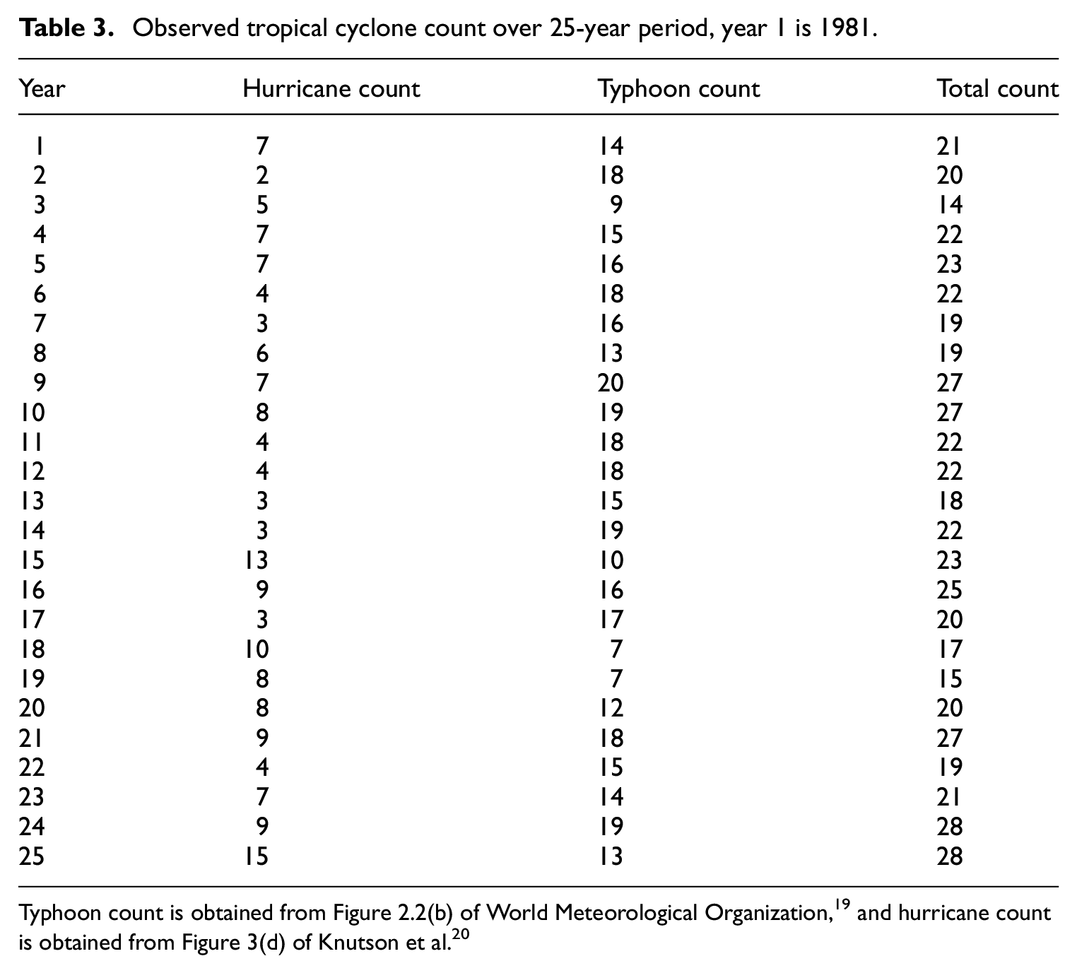
Typhoon count is obtained from Figure 2.2(b) of World Meteorological Organization, ¹⁹ and hurricane count is obtained from Figure 3(d) of Knutson et al. ²⁰

Figure 3.

Observed tropical cyclone count over 25-year period, year 1 is 1981. The figure is obtained from Table 3.

Required for this work are seawater physical properties such as density, specific heat, and volumetric thermal expansion. Safarov et al. ²¹ provide experimental data of physical properties of seawater at different pressures and temperatures. Safarov et al. defines thermal expansibility as change in volume of seawater in response to change in temperature at constant pressure. Values of the thermal expansibility are tabulated in Figure 9 of Safarov et al. Therefore, thermal expansibility as defined is equal to cubical thermal expansion, which is also equal to volumetric thermal expansion. This term, volumetric thermal expansion, will be used in this work instead of thermal expansibility because of its clear indicative nature. The value of the volumetric thermal expansion at atmospheric pressure and average surface temperature is nearly 200 × 10⁻⁶°K⁻¹ as the figure reveals. Seawater-specific heat of 3 980 J kg⁻¹°K⁻¹ and density of 1048 kg m⁻³ are used in the calculations. The depth of the thermohaline brine flow at sea surface is assumed to be equal to the average depth of ocean mixed layers, nearly 95 m based on deBoyer Montégut et al. ²²

Theory and model description

From the “Introduction” and “Background information” sections, a mathematical model of the thermohaline circulation is required for the objectives of this article. Rahmstorf ²³ and Till ²⁴ summarize the current state of understanding of the thermohaline circulation and how it is driven; it is an active research subject. Sandström’s theorem, as explained by Defant, ²⁵ remains a plausible explanation, and the thermohaline circulation is a heat engine that may be represented by a Carnot cycle. Based on Sandström experiments on water tanks, a deep source of heat is required to drive the thermohaline circulation. Of interest for this work is the governing dynamics of the thermohaline circulation at the surface of the oceans. This subject is discussed by Kurtz ²⁶ who proposes the thermosyphon loop principle as a thermodynamic engine cycle. Although Kurtz does not specify the source of heat supply into the cycle, it will be demonstrated that the earth’s internal heat transferred to the oceans is the heat supply: Rahmstorf ²⁷ reveals that the oceans conveying the thermohaline circulation have inverted temperature profiles, and the profiles decrease with the depth measured from surface water. This, however, is not necessarily always valid for other closed or semi-closed water bodies. These bodies have negligible impact on the flow of the thermohaline circulation anyway and may be neglected.

A decrease in ocean temperature with depth yields a negative temperature gradient between deep ocean and surface. Therefore, the earth’s internal heat to the ocean cannot diffuse or convect directly, upward, from ocean floor to the surface. ¹³ The earth’s internal heat to the oceans has to be exchanged in full with the thermohaline brine adhering to ocean floors, and transported southward where the thermohaline brine turns direction upward. There, the brine expands thermally by the exchanged earth’s internal heat. Assuming this heat to be about the same through the oceanic and continental lithospheres, the value of the earth’s internal heat to the oceans is nearly equal to 70% of the total heat produced in the earth’s core of 1.5 × 10²¹ J yr⁻¹. ²⁸ Using 30 Sverdrup (Sv) for the thermohaline brine flow rate ²⁹ and 1048 kg m⁻³ for brine density (see “Data and method” section), the annual circulation rate of the thermohaline circulation is 9.72 × 10¹⁷ kg yr⁻¹, where 1 Sv = 1.0 × 10⁶ m³ s⁻¹. For brine-specific heat of 3 980 J kg⁻¹°K⁻¹ (see “Data and method” section), the earth’s internal heat increases the temperature of the southern oceans by 0.27°K. Using brine volumetric thermal expansion of 200 × 10⁻⁶°K⁻¹ (see “Data and method” section), and average ocean depth of 3000 m, ³ the thermal expansion of the southern oceans is 16.30 cm above the northern oceans. This is close to the observed 20 cm, as discussed in the “Introduction” section. Therefore, the earth’s internal heat to the oceans is the deep source of heat predicted by Sandström. The difference in sea level between the southern and northern hydrospheres drives by gravity the thermohaline circulation at the surface poleward, from south to north. For this work, the observed difference of 20 cm is used as an average value of the available liquid-level difference that drives the thermohaline circulation at the surface.

At the surface, open channel flow equations may be used to parameterize brine flow. Murdock ¹⁴ and Peter ¹⁵ propose for open channel flow V = (8 R_h h_f g/f L)^0.5, where V is average velocity of the liquid in the channel, R_h is hydraulic radius of the channel, h_f is change in liquid elevation in the direction of the flow, g is gravity acceleration, f is friction factor of the channel flow, and L is the length of the channel. The volumetric flow rate may be calculated by multiplying the velocity by the cross-section area of the channel. For the thermohaline circulation, this section varies at the surface from one geographic location to another. For the calculated and observed average value of the flow rate of the thermohaline circulation, average cross-section may be used and the volumetric flow rate Q=A (8 R_h h_f g/f L)^0.5, where A is average cross-section area of the thermohaline brine flow. The hydraulic radius, R_h, is equal to that of the average cross-section of the thermohaline brine flowing at the surface similar to a river flow.

Because seasonal variations change the temperatures of the hemispheres, the ocean mixed layers expand and contract seasonally. As a result, the values of h_f are virtually cyclical and repeatable with time. Therefore, the poleward heat transport has cyclical and repeatable values with time as well. This produces seasonal energy cycles between the hemispheres that drive seasonal tropical cyclones. The same must be true for the ongoing climate change for it induces long-term temperature differences between the hemispheres, and climate energy cycles may thus be expected. As a result of the simultaneous existence of seasonal and climate energy cycles, interaction between them may be expected as well, and this interaction may be modeled mathematically.

It should be noted that variation in the flow rate of the thermohaline circulation with respect to its average value is what is needed for this work. Therefore, the value of h_f only is required because it varies with the seasons and climate. The rest of the variables in the flow rate equation remain about the same and may be canceled out in the mathematical division step. Illustration examples are presented in the “Sample calculations” section.

Related models

Solar model

Swedan ³⁰ provides sources, data, and information used in this section. The average value of the optical depth of the atmosphere (atmospheric air plus clouds) is equal to 0.107. The incident solar energy on the earth viewed as a disc from the sun is 5.51 × 10²⁴ J yr⁻¹. About 30% of this energy is reflected to outer space. Therefore, the solar radiation that penetrates into the atmosphere is equal to 3.86 × 10²⁴ J yr⁻¹. Using the Beer−Lambert Law representation, equation (5) of Swedan, the atmospheric air and clouds absorb 3.92 × 10²³ J yr⁻¹. Just like tropical cyclones, the earth (atmosphere plus surface) removes the absorbed solar heat by evaporating water, which is equal to the latent heat of condensing 953 mm of rain annually. As a result, the annual heat absorbed by the earth is equal to 1.20 × 10²⁴ J yr⁻¹, equation (4) of Swedan. Neglecting land for it has a small thermal capacity, the solar heat absorbed by surface water is thus equal to 1.20 × 10²⁴-3.92 × 10²³ = 8.08 × 10²³ J yr⁻¹. This heat is absorbed unevenly by the mixed layers of the hydrospheres for they have different surface areas. The Visual Encyclopedia of Earth ³ reveals that the percentage of land on the surface of the earth is about 30% of the total surface area. It is unevenly distributed between the hemispheres. About two-thirds of the earth’s land is in the northern hemisphere and 80% of the southern hemisphere is covered with water. The ratio between surface water area of the southern hemisphere to that of the northern hemisphere is thus equal to 1.33 to 1.0. Or, 57.1% of the total water surface is in the southern hemisphere and the remaining 42.9% is in the northern hemisphere. Therefore, nearly 57.1% of the heat absorbed by the mixed layers of the hydrospheres, or 4.62 × 10²³ J yr⁻¹, is absorbed by the southern hydrosphere. The balance, 3.46 × 10²³ J yr⁻¹, is absorbed by the northern hydrosphere. Consequently, the heat distributed at the surface between the southern and northern hemispheres by the thermohaline circulation is equal to (4.62 × 10²³ − 3.46 × 10²³) / 2 = 5.80 × 10²² J yr⁻¹. Also, this heat is equal to the solar heat transported by the thermohaline brine at the surface poleward, from south to north. It is equal to 1.84 PW (petawatt); 1 PW is equal to 1.0 × 10¹⁵ J s⁻¹. This value of heat transport by the thermohaline circulation is equal to the observed and calculated poleward heat transport. Bryden ¹⁷ obtained for the poleward heat transport 2.0 PW, and Macdonald and Wunsch ¹⁸ calculated 1.5 ± 0.3 PW at 24°N. Therefore, the average value of 5.52 × 10²² J yr⁻¹ will be used as average heat transport from the southern hemisphere to the northern hemisphere.

The calculated poleward heat transport of 5.80 × 10²² J yr⁻¹ and observed average value of 5.52 × 10²² J yr⁻¹ will now be compared with the poleward heat transport by air circulation. For simplicity, the average temperature of the thermohaline brine at water surface may be assumed to be equal to the average surface temperature of nearly 287°K. ² This temperature may be assumed to decrease to about freezing temperature at the higher latitudes of the northern hemisphere, where the thermohaline circulation sinks into the abyss. Cooling of the thermohaline brine by air circulation is therefore nearly equal to 13.84°K. For brine-specific heat of 3980 J kg⁻¹°K⁻¹ (see “Data and method” section), and annual thermohaline circulation rate of 9.72 × 10¹⁷ kg yr⁻¹ calculated under the “Theory and model description” section, the poleward heat transport by air circulation is equal to 5.40 × 10²² J yr⁻¹. This value compares well with the calculated and observed values of the poleward heat transport at the surface. The solar model is thus correct.

Hydraulic model

The thermohaline brine at the surface is assumed to flow as a river or fluid in an open channel. Based on the open channel discussion under the “Theory and model description” section, these equations are assumed to apply for the thermohaline brine at the surface

$$\mathrm{Q}=\mathrm{A}{(8{\mathrm{R}}_{\mathrm{h}}{\mathrm{h}}_{\mathrm{f}}\mathrm{g}/\mathrm{f}\mathrm{L})}^{0.5}$$

(1)

$$\mathrm{\Delta }{\mathrm{h}}_{\mathrm{f}}=\beta \left(\frac{{\mathrm{V}}_{\mathrm{m}}}{{\mathrm{A}}_{\mathrm{m}}}\right)({\mathrm{T}}_{\mathrm{SH}}-{\mathrm{T}}_{\mathrm{NH}})$$

(2)

$${\mathrm{d}}_{\mathrm{m}}=\frac{{\mathrm{V}}_{\mathrm{m}}}{{\mathrm{A}}_{\mathrm{m}}}$$

(3)

where Q = average volumetric flow rate of the thermohaline brine at the surface (m³ s⁻¹); A = average cross-section area of the thermohaline flow at the surface (m²); R_h = average hydraulic radius of the thermohaline flow (m); h_f = available average liquid elevation (0.2 m); g = gravity acceleration (m s⁻²); f = friction factor of the thermohaline flow, dimensionless; L = length of the path of the thermohaline flow (m); β = seawater volumetric thermal expansion, 200 × 10⁻⁶°K⁻¹; V_m = volume of the ocean mixed layers (m³); A_m = area of the hydrosphere (m²); d_m = average depth of the ocean mixed layers, 95 m; T_SH = average surface temperature of the southern hemisphere (°K); and T_NH = average surface temperature of the northern hemisphere (°K).

If the flow of the thermohaline brine decreases, the poleward heat transport decreases and the northern hemisphere loses heat. The southern hemisphere gains this heat. They are equal in absolute value at all times, but their net total must be equal to zero for they have opposite convention signs. The available average liquid elevation, h_f, is equal to the net difference in seawater level in the direction of the flow of the thermohaline circulation, from south to north. It is approximately equal to the observed level difference between the southern and northern hydrospheres (0.2 m), as discussed in the “Introduction” section. The assigned values for seawater volumetric thermal expansion and average depth of the ocean mixed layer are based on data sources, as discussed in the “Data and method” section.

Sample calculations

To produce the last column of Table 1, average poleward heat transport and monthly average temperatures of the hemispheres are required. For January, the temperature of the northern hemisphere is 7.93°C and the temperature of the southern hemisphere is 16.36°C. The entire ocean mixed layers of the hyrdospheres may be assumed to expand and contract with seasonal variations for they are mixed within 0.5°K of sea surface temperature. For the mixed layers, brine volumetric thermal expansion is β = 200 × 10⁻⁶°K⁻¹ (see “Data and method” section). The ocean mixed layers average depth, d_m, is about 95 m (see “Data and method” section). Therefore, the temperature difference between the southern and northern hemispheres (T_SH − T_NH) is 8.43. From equation (2), variation in the available liquid elevation is Δh_f = 200 × 10⁻⁶ × 95 × 8.43 = 0.16 m. Using 5.52 × 10²² J yr⁻¹ for average annual poleward heat transport (see “Solar model” section), the monthly average poleward heat transport is 4.60 × 10²¹ J month⁻¹. For 0.2 m average liquid elevation (see “Theory and model description” and “Introduction” sections), variation in the poleward heat transport for the month of January with respect to the average value may be calculated by equation (1) as follows

$$\begin{array}{c}\multicolumn{1}{c}{[{\{8{\mathrm{R}}_{\mathrm{h}}(0.2+0.16)\mathrm{g}/\mathrm{f}\mathrm{L}\}}^{0.5}-{\{8{\mathrm{R}}_{\mathrm{h}}0.2\mathrm{g}/\mathrm{f}\mathrm{L}\}}^{0.5}]/{[8{\mathrm{R}}_{\mathrm{h}}0.2\mathrm{g}/\mathrm{f}\mathrm{L}]}^{0.5}\times 4.60\times 10^{21}}\\ \multicolumn{1}{c}{=[{\{(0.2+0.16)/0.2\}}^{0.5}-1]\times 4.60\times 10^{21}=1.57\times 10^{21}\mathrm{J}}\end{array}$$

The month of January experiences an increase in the poleward heat transport by nearly 34.2% with respect to the monthly average value. Therefore, the northern hemisphere gains 1.57 × 10²¹ J and the southern hemisphere loses 1.57 × 10²¹ J. At the value of average poleward heat transport used, the thermohaline flow rate is nearly 28.56 Sv instead of 30 Sv proposed by Munk and Wunsch. ²⁹ Therefore, average thermohaline flow rate is nearly 38.3 Sv for January.

Similarly, for the month of August, the temperature of the northern hemisphere is 20.99°C and the temperature of the southern hemisphere 10.61°C. Therefore, the temperature difference between the southern and northern hemispheres (T_SH − T_NH) is −10.38. From equation (2), variation in the available liquid elevation is Δh_f = 200 × 10⁻⁶ × 95 × (−10.38) = −0.197 m. Variation in poleward heat transport for the month of August with respect to the average value may be calculated by equation (1)

$$\begin{array}{c}\multicolumn{1}{c}{[{\{8{\mathrm{R}}_{\mathrm{h}}(0.2-0.197)\mathrm{g}/\mathrm{f}\mathrm{L}\}}^{0.5}-{\{8{\mathrm{R}}_{\mathrm{h}}0.2\mathrm{g}/\mathrm{f}\mathrm{L}\}}^{0.5}]/{[8{\mathrm{R}}_{\mathrm{h}}0.2\mathrm{g}/\mathrm{f}\mathrm{L}]}^{0.5}\times 4.60\times 10^{21}}\\ \multicolumn{1}{c}{=[{\{(0.2-0.197)/0.2\}}^{0.5}-1]\times 4.60\times 10^{21}=-4.06\times 10^{21}\mathrm{J}}\end{array}$$

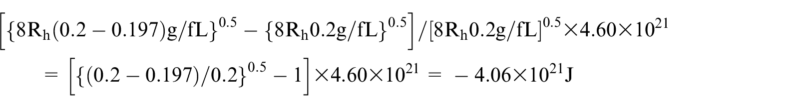
The month of August experiences a decrease in the poleward heat transport by nearly 88.2% with respect to the monthly average value. Therefore, the northern hemisphere loses 4.06 × 10²¹ J and the southern hemisphere gains 4.06 × 10²¹ J. The average thermohaline flow rate is nearly 3.4 Sv for August.

The procedure may be repeated for climate change. The northern hemisphere has warmed more than the southern hemisphere by nearly 0.25°K, as discussed in the “Background information” section and the “Data and method” section. Therefore, T_SH − T_NH = −0.25. Equation (2) gives a reduction in the available liquid elevation, Δh_f, of approximately 200 × 10⁻⁶ × 95 × (−0.25) = −0.0048 m. From equation (1), the climate decreases the flow rate of the thermohaline circulation with respect to the average value by

$$\begin{array}{c}\multicolumn{1}{c}{[{\{8{\mathrm{R}}_{\mathrm{h}}(0.2-0.0048)\mathrm{g}/\mathrm{f}\mathrm{L}\}}^{0.5}-{\{8{\mathrm{R}}_{\mathrm{h}}0.2\mathrm{g}/\mathrm{f}\mathrm{L}\}}^{0.5}]/{[8{\mathrm{R}}_{\mathrm{h}}0.2\mathrm{g}/\mathrm{f}\mathrm{L}]}^{0.5}\times 100}\\ \multicolumn{1}{c}{=[{\{(0.2-0.0048)/0.2\}}^{0.5}-1]\times 100=-1.20\%}\end{array}$$

This yields a reduction in the poleward heat transport of −6.62 × 10²⁰ J yr⁻¹, approximately −5.52 × 10¹⁹ J month⁻¹, which may be assumed to have the same value for all months for the near future. The northern hemisphere loses this heat every month and simultaneously the southern hemisphere gains this heat. Referring to Table 2, at the conclusion of a 6-year climate energy oscillation, the cumulative variation in the heat of the northern hemisphere for the month of January is equal to 1.57 × 10²¹-5.52 × 10¹⁹ × 72 = −2.41 × 10²¹ J. The heat budget of the southern hemisphere increases by 2.41 × 10²¹ J. For the month of August, the heat deficit of the northern hemisphere is equal to −4.06 × 10²¹-5.52 × 10¹⁹ × 72 = −8.03 × 10²¹ J, and the heat budget of the southern hemisphere increases by 8.03 × 10²¹ J.

Similarly, referring to Table 2, for a 10-year climate energy oscillation, the northern hemisphere experiences in the month of January heat deficit of 1.57 × 10²¹-5.52 × 10¹⁹ × 120 = −5.05 × 10²¹ J. Simultaneously, the heat budget of the southern hemisphere experiences an increase of 5.05 × 10²¹ J. For August, the northern hemisphere heat deficit is −4.06 × 10²¹-5.52 × 10¹⁹ × 120 = −1.07 × 10²² J, and the southern hemisphere heat budget increases by 1.07 × 10²² J.

At the conclusion of a 6-year energy cycle, the heat budget deficit in the northern hemisphere is equal to −5.52 × 10¹⁹ × 72 = −3.97 × 10²¹ J, and the heat budget surplus in southern hemisphere is 3.97 × 10²¹ J. A 10-year climate energy cycle leaves at the conclusion of the 10th year heat budget deficit of −5.52 × 10¹⁹ × 120 = −6.60 × 10²¹ J in the northern hemisphere and heat budget surplus of 6.60 × 10²¹ J in the southern hemisphere.

Discussion and conclusion

Seasonal variations in the temperatures of the hemispheres are caused by the motion of the earth around the sun. Their average values are tabulated in Table 1 based on data sources discussed under the “Data and method” section. In January, the average temperature of the northern hemisphere reaches a minimum value of 7.93°C, well below the average surface temperature of the earth of nearly 14°C. For this month, the temperature of the southern hemisphere is 16.36°C. It is greater than the average surface temperature. As a result, surface water contracts in the northern hemisphere and expands in the southern hemisphere. Therefore, the available liquid elevation for the thermohaline circulation increases by 0.16 m with respect to the average value of 0.2 m, and the poleward heat transport exceeds its average monthly value by 1.57 × 10²¹ J. The poleward heat transport for January is nearly 34% greater than the average monthly poleward heat transport of 4.60 × 10²¹ J month⁻¹. Between February and April, the temperature of the northern hemisphere increases and the temperature of the southern hemisphere decreases. The change in liquid elevation with respect to the average value decreases and the poleward heat transport decreases as well. In April, the average temperatures of the hemispheres are about equal. For this month, the change in the available liquid elevation is nearly equal to zero and variation in the poleward heat transport is small and negligible. Therefore, in April, there is no significant variation in the poleward heat transport, and this month observes the average value of 4.60 × 10²¹ J month⁻¹.

The scenario changes in the succeeding months. Between May and August, the average temperature of the northern hemisphere is now greater than that of the southern hemisphere. Changes in liquid elevation are thus less than zero, and variations in the monthly poleward heat transport are in the negative field. The value of the monthly poleward heat transport decreases steadily, and in the month of August, it reaches a minimum value of nearly 12% of its average monthly value. Thereafter, the poleward heat transport increases and the cycle repeats.

Variation in the poleward heat transport is equal to the energy exchanged between the hemispheres. As mentioned in the “Hydraulic model” section, if the poleward heat transport decreases, the northern hemisphere loses heat and the southern hemisphere gains this heat. They are equal in absolute value but have opposite convention signs. This is illustrated in Figure 1. Variation in the monthly heat exchanged with the northern hemisphere of this figure is equal to the variation in the monthly poleward heat transport presented in the last column of Table 1. The monthly heat exchanged with the southern hemisphere is a mirror image of that of the northern hemisphere with respect to the horizontal coordinate. The variations in the monthly poleward heat transport having negative signs in the last column of Table 1 are monthly heat transported from the northern hemisphere to the southern hemisphere. Their total sum of −1.46 × 10²² J is equal to the energy that drives tropical cyclones; it is nearly equal to 27% of the annual poleward heat transport.

Emanuel et al. ³¹ estimated the number of observed storms between 1980 and 2005 to be nearly 1690, approximately 68 events annually worldwide. Storm energy varies between 1.3 × 10¹⁷ J day⁻¹ and 5.2 × 10¹⁹ J day⁻¹. ³² Based on National Oceanic and Atmospheric Administration, storm durations may be between 5 and 25 days. Therefore, the total annual energy depleted by the storms is between 8.9 × 10²¹ J yr⁻¹ and 2.7 × 10²² J yr⁻¹. The calculated annual energy of 1.46 × 10²² J yr⁻¹ falls well within the observed range.

The calculated variation in the flow rate of the thermohaline circulation during the year is large, between 3.4 and 38.3 Sv (see “Sample calculations” section). Srokosz and Bryden ⁴ observed considerable interannual fluctuation in the Atlantic Meridional Overturning Circulation (AMCO), between 3 and 39 Sv. They are in good agreement.

Based on Figure 1 and Table 1, the poleward heat transport reaches its minimum value in the month of August, and then reverses and begins to increase. It is thus reasonable to consider the month of August as a month defining the end of seasonal heat supply to the southern hemisphere and beginning of seasonal heat supply to the northern hemisphere. The geographic configuration of the hydrosphere suggests that the energy of hurricanes may be a function of the magnitude of variation in the solar heat with respect to the average value of the northern hemisphere. The energy of typhoons may be a function of the magnitude of solar heat variation in the southern hemisphere. Therefore, the heat required for seasonal typhoons may be equal to the sum of the monthly variation in the poleward heat transport between May and August, which is equal to −9.38 × 10²¹ J. The heat required for seasonal hurricanes may be equal to the sum of the monthly variation in the poleward heat transport between August and October, which is equal to −5.19 × 10²¹ J. The minus is a convention sign indicating that heat is being transferred southward, from the northern hemisphere to the southern hemisphere. Uneven surface warming caused by the climate appears to alter the natural seasonal variations of energy between the hemispheres as Figure 2 reveals. Because the northern hemisphere has been warming more than the southern hemisphere, the available liquid elevation for the thermohaline flow has decreased by 0.0048 m as calculated in the “Sample calculations” section. The flow rate of the thermohaline circulation has therefore decreased, which is observed. Srokosz and Bryden ⁴ observed decreasing trend in the flow rate of AMCO. As a result of the decrease in the flow rate of the thermohaline circulation, the northern hemisphere transfers to the southern hemisphere about 5.52 × 10¹⁹ J every month, which has to be accounted for. These transfers add cumulatively with time. For this discussion, 6- and 10-year climate oscillations are considered. At the conclusion of each oscillation period, there remains a substantial amount of energy in each hemisphere with the convention sign, and natural average conditions are not within reach. The 6-year oscillations leave in the southern hemisphere a heat budget surplus of approximately 4.0 × 10²¹ J at the conclusion of the sixth year (see “Sample calculations” section). Simultaneously, the northern hemisphere has a heat deficit of −4.0 × 10²¹ J. The heat budget variations are higher for 10-year oscillations, nearly 6.60 and −6.60 × 10²¹ J for the southern and northern hemispheres, respectively. The heat added to the southern hemisphere is large enough to prime the atmosphere and cause it to depart from average conditions. Similar to tropical cyclones, heat and temperature difference between surface water and air is required. The heat is available, and the highest temperature variation in the southern hemisphere occurs in the southern hemispheric summer. The basic requirements for thermodynamic transformation to occur are thus satisfied. The transformation is in essence a thermodynamic heat engine, similar to tropical cyclones. Large-scale water evaporation or El-Niño or equivalent events are, therefore, likely to occur toward the end of the year during the southern hemispheric summer based on Table 1. The produced air circulation transfers most of the latent heat of water evaporation from the southern hemisphere to the northern hemisphere. The displaced drier air flows from the northern hemisphere to the southern hemisphere. While the northern hemisphere experiences a wetter climate than average, the southern hemisphere experiences a drier climate. At the conclusion of this event, variation in the heat content of each hemisphere approaches zero value and natural average conditions are reached. The climate-induced oscillations then repeat all over again.

It is not a coincidence that most of tropical cyclones and El-Niño or equivalent events travel poleward to the northern hemisphere. The majority of their heat is dissipated in the northern hemisphere as latent heat of water vapor condensation. This suggests that their heat is originated from the northern hemisphere; specifically, the heat is in essence variation in the poleward heat transport. These events only return the heat back to the northern hemisphere to maintain average conditions.

Because of the repeatable nature of seasonal variations, this work reveals that the total seasonal energy available to tropical cyclones is about the same every year. Therefore, if the energy and count of hurricanes increase, the energy and count of typhoons should decrease and vice versa based on this work. This is observed in the record. Table 3 and Figure 3 present the observed number of tropical cyclones between 1981 and 2005. There appears to be an opposite relationship between them: If the number of hurricanes increases, the number of typhoons decreases and vice versa. In addition, the tropical cyclone count has cycle durations of approximately 4 to 8 years, as the figure reveals. The existence of these energy cycles is predicted by the work presented in this article. It is, therefore, reasonable to conclude that there exist climate energy cycles between the hemispheres and the seasonal tropical cyclone count is affected by these cycles. Because the difference in surface temperature between the hemispheres varies with climate change, the magnitude and frequency of energy cycles between the hemispheres may be variable. Figure 3 shows an increasing trend in the total number of seasonal tropical cyclones. This, however, does not necessarily mean an increasing trend in the total energy dissipated by these cyclones. More data and in-depth analysis are required, which is beyond the scope of this work.

The science of calculating and projecting tropical cyclones does not appear to be fully developed. The energy that drives hurricanes and typhoons may be calculated and projected with reasonable accuracy as this parameterization work reveals. This is an important step in the development of this science. Surface temperature trend and seasonal temperature variation are available in the record or can be calculated. Therefore, Table 1, Figure 1, Figure 2, and the figures in between may be produced on daily, monthly, for any desired cycle period, or projected into the future. The magnitude of energy cycles between the hemispheres can thus be determined, which is the fundamental requirement for the analysis of tropical cyclones and their oscillations with time. More scientific observations and data are therefore needed, given the breadth and challenges associated with energy oscillations between the hemispheres. The earth is large in size and includes earth subsystems that interact among one another, which makes this subject multidisciplinary and challenging. This parameterization of energy cycles could narrow down the area of research and may assist earth researchers in obtaining robust and coordinated data to assess tropical cyclone trends in a warming world.