
Abstract
According to the problem that the existing high-speed parallel robot cannot satisfy the operation requirements of non-planar industrial production line, a 6-degrees-of-freedom high-speed parallel robot is proposed to carry out the kinematic and dynamic analyses. Combining with the door-type trajectory commonly used by the parallel robot, it adopts 3-, 5-, and 7-time B-spline curve motion law to conduct the trajectory planning in operation space. Taking the average cumulative effect of joint jerky as the optimization target, a trajectory optimization method is proposed to improve the smoothness of robot end-effector motion with the selected motion law. Furthermore, to solve the deformation problem of the horizontal motion stage of the trajectory, a mapping model between the control point subset of B-spline and the motion point subset of trajectory is established. Based on the main diagonally dominant characteristic of the coefficient matrix, the trajectory deformation evaluation index is constructed to optimize the smoothness and minimum deformation of the robot motion trajectory. Finally, compared to without the optimization, the maximum robot joint jerk decreases by 69.4% and 72.3%, respectively, and the maximum torque decreases by 51.4% and 38.9%, respectively, under a suitable trajectory deformation.
Introduction
High-speed parallel robots are widely used in industrial production lines, such as food industry, pharmaceutical industry, and electronics industry. They are mainly used to complete high-speed sorting, packing, stacking, and assembly. However, the high-speed parallel robots with less degrees of freedom (DOF) cannot meet the complex industrial production requirements. Therefore, the application of 6-DOF high-speed parallel robots is gradually increasing. They have higher requirements for robot motion and hence should be optimized from the aspects of dynamics and trajectory planning to improve the smoothness of motion and inhibit the residual vibration of the robot.1–3
The trajectory planning method of the robot can be divided into two categories according to the space in which it is located, namely, joint space trajectory planning4,5 and operating space trajectory planning.6,7 The trajectory planning in joint space is based on the motion mapping relationship between the operation space and the joint space, and the corresponding motion position sequence of the joint is solved according to the key pose sequence of the end-effector trajectory, so it can achieve better motion smoothness. However, because the motion mapping relation between the joint space and the operating space is usually non-linear, it cannot guarantee that the end of the robot moves strictly according to the given trajectory. Hence, the trajectory planning in operating space is usually used in robot control and actual production.
In terms of the selection of the laws of motion, polynomial laws of motion, trapezoidal acceleration laws, sinusoidal laws of motion, and low-order spline laws are usually adopted.8–10 At present, domestic and foreign scholars have conducted extensive research in this field. For example, Angeles et al. 11 proposed a method for the planning of operating space trajectories using piecewise polynomial functions. Macfarlane et al. 12 combined 5-time polynomial motion law and sinusoidal motion law and proposed a path planning method for robot. The method is connected by sinusoidal movement at the beginning and end of the trajectory, thus reducing the residual vibration at the end of the robot. Liu et al., 13 based on the 7-time B-spline motion law, proposed a method to make the initial and final velocities, accelerations, and jerks of the robot joint freely configured at the same time. In terms of the research on the robot trajectory optimization method, Li et al. 14 planned the hyperactivity curve of the trajectory based on sinusoidal and linear motion laws and then obtained the modified s-shaped motion law. Based on the motion law of B-spline, Sencer et al. 15 considered the minimum trajectory motion error as the index to obtain the optimal motion trajectory. Rew and Kim 16 and Ha et al. 17 proposed the concept of the rate coefficient of sudden change of degree for the deceleration phase of the trajectory so as to construct an asymmetric s-curve movement rule for reducing the robot vibration.
In most of the above mentioned trajectory planning and optimization methods, the B-spline motion law is widely used in the actual process. Because, on the one hand, it can effectively reduce the motion parameters required by the robot, on the other hand, more than 5-time B-spline it can achieve the curve smoothness of the robot acceleration and jerk to reduce the vibration in the movement.18–20 However, regarding parallel robot, the previous trajectory planning method based on high-order B-spline motion law is seldom studied. Especially when the parallel robot moving platform has 6 DOF simultaneously in the working space, whether the B-spline motion law can meet the motion trajectory planning requirements of the robot joint space is still unclear. Hence, the relevant solution and analysis of the 6-DOF parallel trajectory planning method are necessary to be deepened in terms of the motion parameters and deformation error.
This article is organized as follows: Section “Kinematic analysis” introduces the 6-DOF high-speed parallel robot and builds the kinematic model of the parallel robot. In section “Dynamic analysis,” according to the virtual work principle, the dynamic model of the parallel robot is illustrated. Section “Trajectory description” describes the pick-place trajectory curve commonly used by parallel robot in the production line. Section “The k time B-spline curve motion law” introduces the B-spline curve motion law and the computing method. Section “The trajectory planning in the joint space and the operating space,” adopting 3-, 5- and 7-time B-spline curve motion law, simulates and analyzes the trajectory curve situation in the joint space and operation space. In section “ The trajectory optimization in the operating space,” according to the problems generated by the above procedure, an optimization method for 5- and 7-time B-spline curve is proposed. Finally, a summary and future prospects are detailed in section “Conclusion.”
Kinematic analysis
The 6-DOF parallel robot is shown as in Figure 1, and it consists of a static platform, a moving platform, and six identical independent kinematic chains. Each kinematic chain is the RSS (R for revolute joint, S for spherical joint) construction, which has a motor, a reducer, a master arm, a slave arm, and two spherical joints. The master arm produces rotation movement driven by the motor. The slave arm is driven by the spherical joint mounted at the end of the active arm. The other end of the slave arm is connected to the moving platform. Through the six independent kinematic chains, the robot’s moving platform can achieve 6 DOF in space, namely, three translational motions and three rotational motions.

The structure diagram of the 6-DOF parallel robot.
Because the six kinematic chains have almost identical structures, the reference frame is defined as shown in Figure 2. The coordinate frame O-xyz is attached to the static platform, and the coordinate frame P-uvw is attached to the moving platform. 21 Therefore, the closed-loop position vector equation in the ith kinematic chain is expressed as

where

The meaning of the kinematic parameters used in the above equation is illustrated in Table 1.
Meaning of the kinematic parameters.


Vector diagram of a kinematic chain.
The inverse kinematics model can be obtained by equation (1), and the rotation angle of robot joint is shown as follows

where
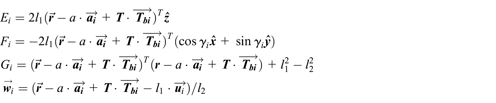
Taking the derivative of equation (1) with respect to time, the joint velocity equation can be obtained as follows

where
Equation (3) can be rewritten as follows

where


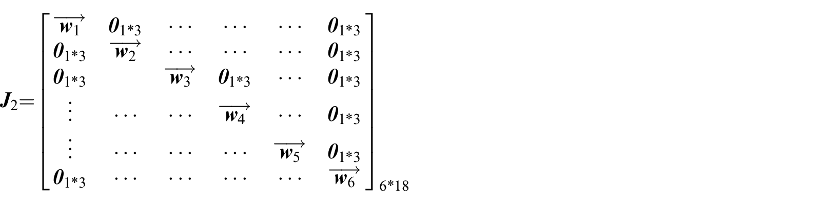


Jacobian matrix
Taking the quadratic derivative of equation (1) with respect to time, the joint acceleration equation can be obtained as follows

where
Taking the third derivative of equation (1) with respect to time, the joint jerk equation can be obtained as follows

where
Dynamic analysis
Since the motion branch chain of the 6-DOF parallel robot is controlled independently, the local coordinate system Oi-xiyizi on each chain should be established when building the dynamic model. The origin Oi of the local coordinate system is at the center of mass of the slave arm, the zi axis always points to the axis direction of the slave arm, the xi axis is located in the plane formed by
According to the virtual work principle and ignoring the friction, the dynamic equation of the parallel robot can be obtained as follows

where


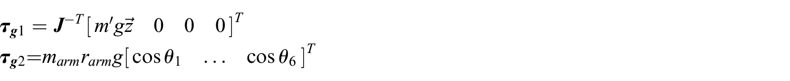


where
The meaning of the dynamic parameters used in the above equation is illustrated in Table 2.
Meaning of the dynamic parameters.

Trajectory description
As the 6-DOF parallel robot is mainly used to complete the grasping and placing operations in practical engineering (Figure 3(a)), the typical motion mode of the end movement platform in the working space is point-to-point (PTP) motion, and it requires some certain obstacle avoidance points. And the specified motion trajectory of the parallel robot in the working space is shown in Figure 3(b). Ow-xwywzw is the local coordinate system that the coordinate O-xyz translates (H+h) −hd along the negative direction of the z axis, and the parameters of the trajectory are defined in Table 3. Hence, the robot motion trajectory is a “door” type including the rising section p0-p7, the horizontal section p7-p8 (the central point of the horizontal section is p3), and the descending section p8-p6.

Schematic of the motion trajectory in workspace.
Meaning of the trajectory curve parameters.

In order to make the trajectory more compliant and reduce the impact and time consumption of the inflection on the robot motion, the mixed movement sections p1-p2 and p4-p5 are established. In addition, the standard trajectory adopted has an ha of 0.025 m and ba of 0.7 m. The maximum movement velocity of the robot is 120 times/min, so the optimal trajectory time is 0.25 s.
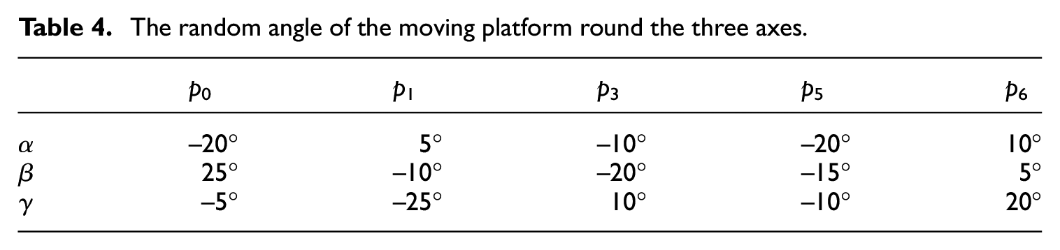
In addition, the randomly set rotation angles of the moving platform are added when the robot moves along the trajectory to verify the impact of the rotation angles of the dynamic platform on the trajectory planning. Since the specified moving platform does not rotate more than ±30° around the three coordinate axes, the random rotation angle can be set as shown in Table 4.
The random angle of the moving platform round the three axes.
The k-time B-spline curve motion law
For the robot trajectory curves to maintain smoothness, the k-time B-spline curve motion law is adopted in this article. According to the above trajectory description,
22
it selects the five key points, including p0, p1, p3, p5, and p6, to obtain the five-group point-time series
First,
Second,

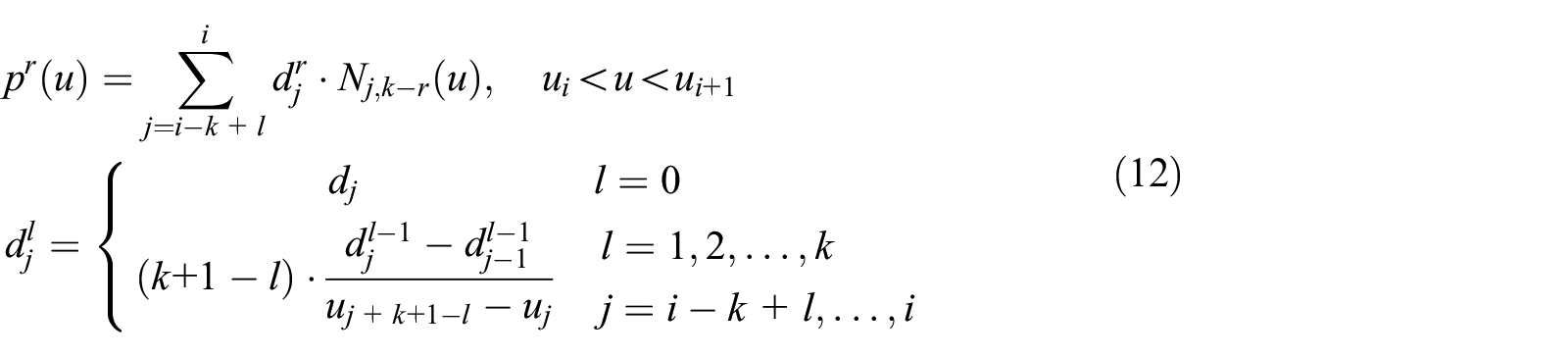
Third, the B-spline curve equation can be shown as follows

where

where the r derivative equation of
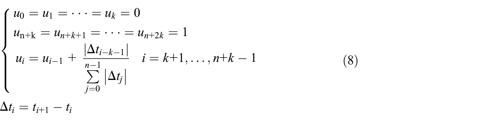
Fourth, the control vertices should be solved first, and the solution equation set is shown as follows

where


where

Fifth, for the k-time B-spline curve, it must also increase k – 1 boundary conditions, which can be obtained by tangent vector boundary conditions. Due to the repeat times k on both ends, the k-time B-spline curve at the end of the first control vertex is at the end of the first data point, so the following k – 1 boundary conditions can be obtained
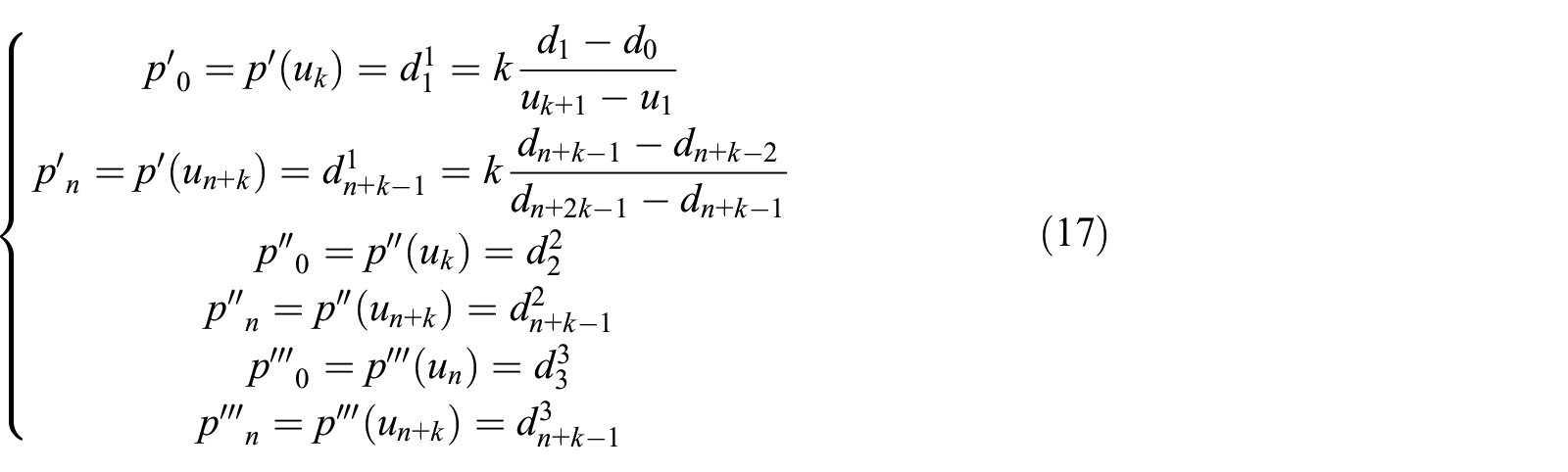
Finally, according to equations (8) and (9), the basis function can be calculated, and through equations (11) and (12), the control vertices can be obtained. Therefore, the position, velocity, acceleration, and jerk of the robot end-effector can be calculated using the B-spline curve equation (13). Then, through the kinematic inverse solution, the motion parameters of the robot joint can be obtained and a similar trajectory can be implemented.
The trajectory planning in the joint space and the operating space
In the joint space, by adopting the B-spline curve motion law, the trajectory curves of the robot end-effector without the rotation motion of the moving platform are shown in Figure 4. It shows that for different B-spline curve motion laws, although each trajectory can strictly pass the given trajectory points, there are slight differences between the trajectories, among which the maximum error of each trajectory in the direction of the extension z axis is about 9.4 mm. Meanwhile, as trajectory planning in joint space relies on the kinematic forward solution, the process to calculate the position is non-linear. Therefore, it will lead to deformation of robot end trajectory curve, which will have certain influence on robot motion.
The trajectory curve of different B-spline curve motion laws in the joint space without the rotation angle of the moving platform.
In addition, when the moving platform produces rotation motion, the trajectory curves of different B-spline curve motion laws in joint space are shown in Figure 5. Then, when the robot end-effector produces arbitrary angular motion, the non-linear effect will aggravate the deformation of the movement curve of the robot end-effector and produce irregular path changes. In the actual operation process, this situation will easily lead to the random motion of the robot, which will cause danger to the operation and easily bring about damage to the equipment. Hence, for the multi-DOF parallel robot, the B-spline curve motion rule is not suitable for the trajectory planning in the joint space.

The trajectory curve of different B-spline curve motion laws in the joint space with the random rotation angle of the moving platform.
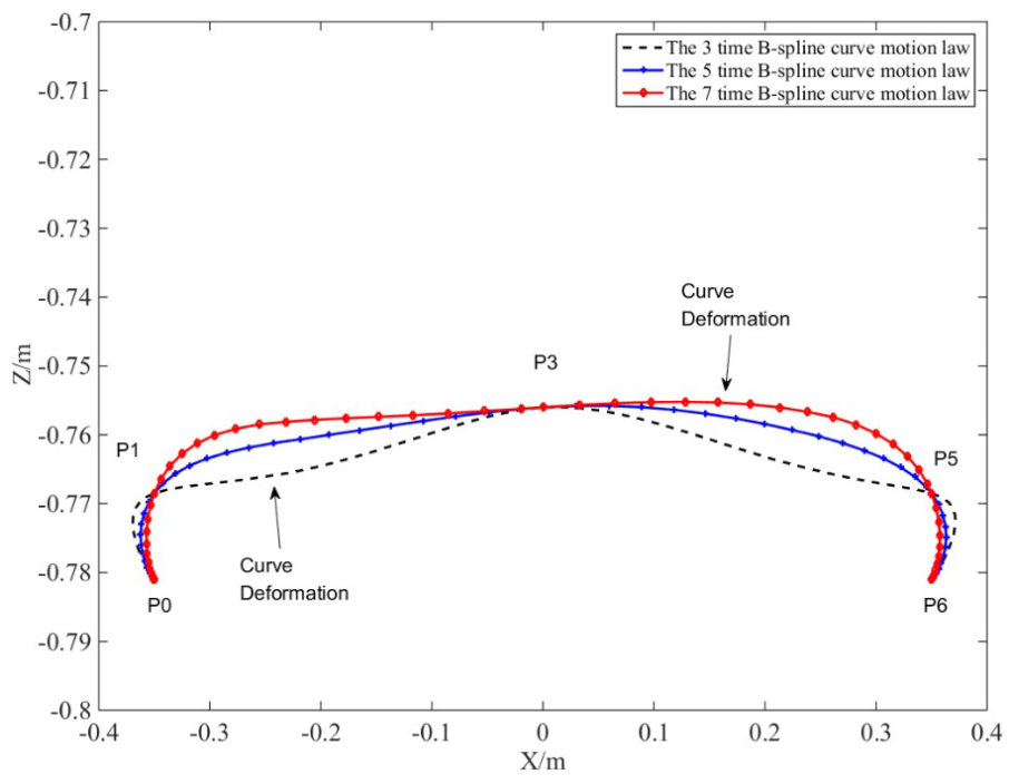
In the operating space, by adopting the above motion analysis method, the motion law of different B-spline curves can be obtained, as shown in Figure 6. It shows that the trajectory curve of the different motion laws is similar. It can also strictly provide trajectory points p0, p1, p3, p5, and p6, and there is no excessive deformation in the curve.

The trajectory curve of different B-spline curve motion laws in the workspace without and with the random rotation angle of the moving platform.
Figure 7 shows that the motion parameters of arbitrary robot active joints are compared and analyzed with different B-spline curve motion laws in workspace. According to Figure 7(a) and (b), the velocity curves of the robot active joint 1 are continuous and smooth with every motion law, but when adopting the 3-time B-spline curve, the starting acceleration of the robot active joint 1 is not equal to 0, the acceleration curve is not smooth, and there exists break point, thus implying that the driving torque provided by the joint motor as shown in Figure 7(d) does not guarantee complete smoothness, and there are sharp points that cause the robot jitter during motion, and the initial acceleration is not equal to 0. In addition, it can be clearly seen that when the 5-time B-spline curve motion law is adopted, the output torque demand provided by the motor is relatively small, reducing the motor consumption.

Comparison motion parameters of the robot joint with different motion laws in workspace: (a) velocity of robot joint 1, (b) acceleration of robot joint 1, (c) jerk of robot joint 1, and (d) torque of robot joint 1.
According to Figures 7(c) and 8, the 5- and 7-time B-spline curve motion law can guarantee the smoothness of jerk curve of the robot joint and end-effector. From these figures, only the jerk curve of the latter can be equal to 0 at start and end points so as to improve the motion stability of robot in the rapid picking and placing motion. However, no matter the joint or the end-effector, the maximum jerk value of the 5-time B-spline curve is less than the 7-time B-spline curve.
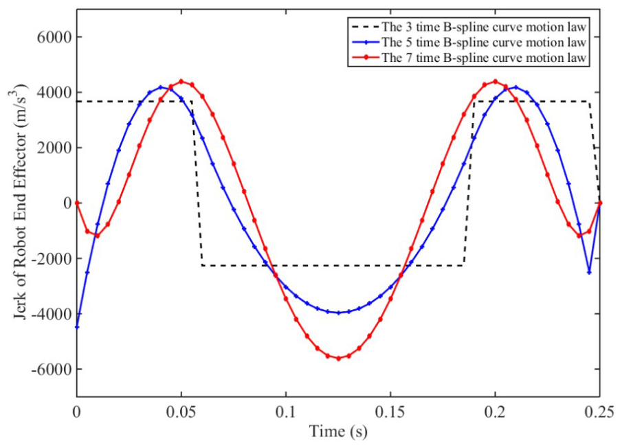
Comparison jerk curve of the robot end-effector with different motion laws in workspace.
In addition, when the robot end-effector produces arbitrary angular motion, the motion curve of the robot end-effector will not be deformed like the joint space trajectory planning, so the workspace trajectory planning is applicable to the 6-DOF high-speed parallel robot, and the 5- or 7-time B-spline curve motion law can be given priority.
The trajectory optimization in the operating space
When performing tasks, robots are usually required to move as fast as possible. However, as the speed of motion increases, the acceleration and jerkiness are usually increased, which is not conducive to the smoothness and accuracy of the motion process. Therefore, it is necessary to optimize the motion track.
As the smoothness of the trajectory is mainly reflected in the value of jerkiness, it is necessary to ensure that it is not too large in the process of robot motion. Therefore, considering the average cumulative effect of the trajectory jerkiness in the process of motion, the following indexes can be defined to evaluate the smoothness of the trajectory

where n is the number of the robot joint and Ttotal is the total motion time. The optimization model of the trajectory can be shown as follows
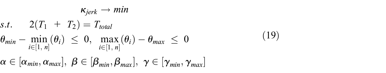

where θmin and θmax are the maximum and minimum range of the robot joint rotation angle, respectively.
The trajectory after minimum jerk optimization.
Table 5 compares the motion parameters of robot joints before and after optimization, and it can clearly see that using the minimum jerk method can effectively reduce the maximum speed, maximum acceleration, maximum jerk, and maximum input torque of the robot joints. In particular, after the optimization, the maximum jerk of the 5- and 7-time B-spline curves is 5.48 × 10⁶°/s3 and 4.25 × 10⁶°/s3, respectively, which is 66.4% and 77.3% lower than the maximum jerk of the previous trajectories. And the input torques of robot joints are also reduced by 36.4% and 37.6%. Thus, the minimum jerk optimization model can obviously reduce the joint consumption during the movement of the robot and improve the smoothness of the trajectory.
Comparison the motion parameters of the robot joint without optimization and after minimum jerk optimization.

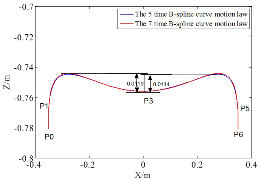
However, no matter the 5- or 7-time B-spline curve motion law, the above optimization method can cause the deformation of the trajectory curve, where the maximum displacement from the trajectory’s highest point to the given trajectory point P3 is 11.4 and 11.9 mm. Hence, it is necessary to analyze the deformation cause of the B-spline curve.
According to the characteristics of the B-spline curve in Figure 10, on the one hand, with the higher order of the spline curve, the generated curve will deviate from its control vertex, as shown in Figure 10(a); on the other hand, when the intermediate control vertex deviates from the start and end points, the distance between the B-spline curve and the control vertex will be longer, as shown in Figure 10(b). Hence, relative to the 3-time B spline curve, when 5- or 7-time B spline curve is adopted to construct the motion trajectory, it is necessary to pay attention to the deformation of the motion trajectory.
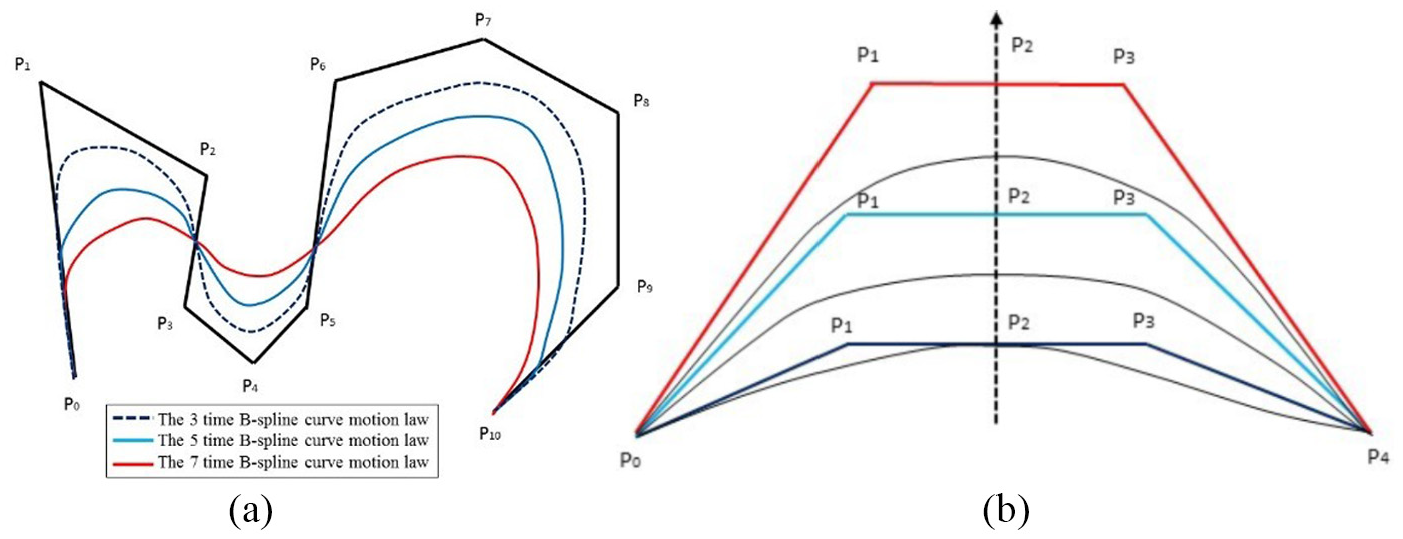
The properties of B-spline curve: (a) closeness of curve to control vertex and (b) impact of control points on curve.
Equation (13) can be rewritten as follows

which means that when the trajectory points
For the k-time B-spline motion law, if the repeatability of both nodes of the node vector U is set as εd =k + 1, then the control vertex number of the B-spline curve is n + k according to the given trajectory

According to the calculation rule of matrix, when calculating the control vertex of k-time B spline trajectory, given the must-pass point sequence

which means that

which indicates that if the effect of the coupling property between the must-pass points needs to be reduced, then the elements beside the main diagonal elements should be set to 0, or when
The eigenvalue analysis of matrix
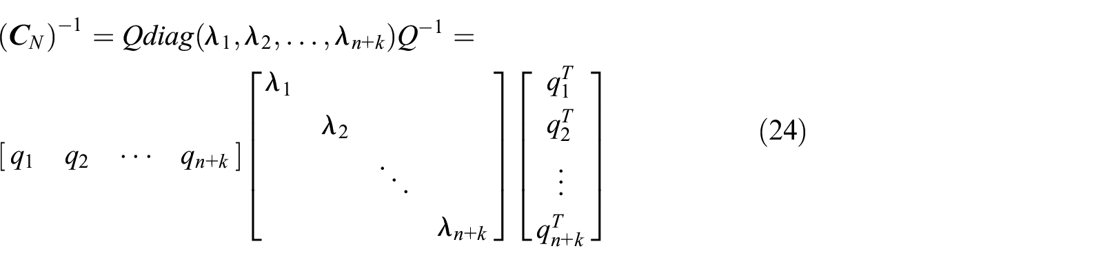
where


According to the subadditivity of the normed linear space and the F norm definition, the following inequality can be obtained

The left-hand side of the inequality can be obtained as follows

where the index of the coupling characteristic of the must-pass points can be defined as follows
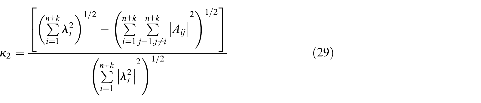
Then, according to the above constraint conditions of the optimization procedure, the minimum deformation index can be defined as follows

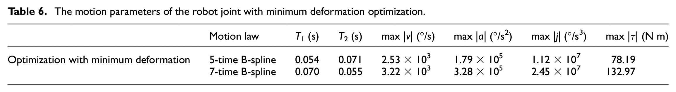
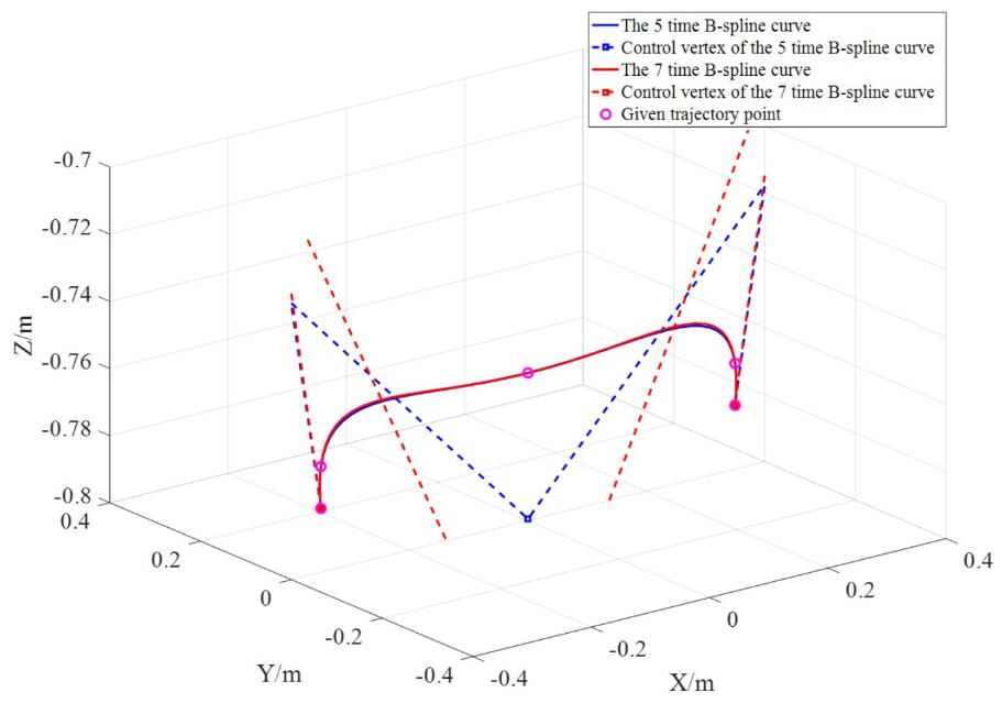
Then combining with constraint situation in equation (19), the minimum deformation optimization result is shown in Figure 11 and Table 6. After the minimum deformation optimization, the deformation distance of the trajectory is significantly lower than that of the trajectory after the minimum jerk optimization, and the control vertex of the former is closer to the given trajectory point, while the control vertex of the minimum jerk optimization is far from the given trajectory point. However, after the minimum deformation optimization, all the motion parameters of the robot joints are much higher than the value of minimum jerk optimization, especially in aspects of maximum jerkiness and maximum input torque of the robot joint. Therefore, in the process of the trajectory optimization, the minimum deformation and smoothness of the robot should be taken into account at the same time.

The motion trajectory after minimum jerk and deformation optimization: (a) the 5-time B-spline curve motion law and (b) the 7-time B-spline curve motion law.
The motion parameters of the robot joint with minimum deformation optimization.
According to the above analysis, combining with the two optimization indices of minimum jerk and minimum deformation, the new optimization index can be redefined as

where

The optimization trajectory and motion parameter results are shown in Figure 12 and Table 7. It shows that although the comprehensive index optimization method simultaneously reduces the trajectory deformation and all motion parameters of the robot joint, the trajectory deformation distance still has a large deviation.

The motion trajectory after comprehensive optimization.
The motion parameters of the robot joint with the comprehensive index.

Hence, it needs to establish an error indictor

The calculation results are shown in Table 8, and it can be seen that as
The relation between

The motion trajectory with the optimum
Conclusion
This article introduces a kind of 6-DOF high-speed parallel robot and analyzes its kinematic and dynamic problem. Then combining with its commonly used trajectory in industrial production line, it proposed the trajectory planning method in operation space to achieve the smoothness and accuracy motion of the robot end-effector, so the conclusion can be summarized as follows:
Because of the non-liner mapping relationship existing in the process of the kinematic forward solution, the B-spline curve motion law is not suitable for trajectory planning in the joint space. It may cause the trajectory curve to deform, especially when the robot end-effector generates rotation motion.
For the trajectory planning in the operation space, the generated motion trajectory can be strictly followed to set the track requirements without deformation, especially the robot end-effector has rotation motion. Through comparison, it can be found that the 5- and 7-time B-spline curve can guarantee that no sharp points occur in the curve of each motion parameters of the robot joints, which is more suitable for 6-DOF high-speed parallel robot than the 3-time B-spline curve.
In the trajectory optimum produce, three optimization methods are analyzed. The minimum joint jerk optimization method can reduce the robot joint jerk by a wide margin, but the trajectory deformation error of the robot increases, which leads to uncontrollable motion of the robot. The minimum trajectory deformation optimization method has the opposite effect. Therefore, a comprehensive optimization method with a minimum joint jerk and trajectory deformation error is presented. Compared to without the optimization, the maximum robot joint jerk decreases by 69.4% and 72.3%, respectively, and the maximum torque decreases by 51.4% and 38.9%, respectively, under a suitable trajectory deformation.
Therefore, this method can improve the stability and smoothness of the robot motion, thereby suppressing the residual vibration. In future work, the space curve trajectory planning method will be further studied to find a curve optimization design method more suitable for the 6-DOF parallel robot.
Footnotes
Declaration of conflicting interests
The author(s) declared no potential conflicts of interest with respect to the research, authorship, and/or publication of this article.
Funding
The author(s) disclosed receipt of the following financial support for the research, authorship, and/or publication of this article: This work was supported by the National Key Technology Research and Development Program of the Ministry of Science and Technology of China (Grant No. 2015BAF11B00).