Sage Journals: Discover world-class research

Abstract

German

Spanish

French

Scientists using laboratory animals are under increasing pressure to justify their sample sizes using a “power analysis”. In this paper I review the three methods currently used to determine sample size: “tradition” or “common sense”, the “resource equation” and the “power analysis”. I explain how, using the “KISS” approach, scientists can make a provisional choice of sample size using any method, and then easily estimate the effect size likely to be detectable according to a power analysis. Should they want to be able to detect a smaller effect they can increase their provisional sample size and recalculate the effect size. This is simple, does not need any software and provides justification for the sample size in the terms used in a power analysis.

Keywords

3Rs ethics and welfare policy reduction sample size statistics techniques

Introduction

There is a crisis in pre-clinical biomedical research involving laboratory animals. Too many papers publish results which turn out to be irreproducible.^1–3 One estimate puts the cost at $28 billion being wasted per annum in the United States alone.⁴

The causes of this irreproducibility crisis have not been fully identified. But it has been known for many years that experiments are often poorly designed, inadequately analysed, and misreported.^5–7 A survey of 271 papers chosen at random involving rats, mice and non-human primates⁸ showed that 87% did not report random allocation of experimental subjects to the treatments and 86% did not report “blinding” when measuring the results. None of the papers gave any justification for their choice of sample size, and a substantial number of papers failed even to state the sex, age or weight of the animals. Such failures can lead to too many false-positive results.⁹ It has also been suggested,¹⁰ on somewhat debatable evidence, that many animal experiments are under-powered, leading to large numbers of false-negative results. If these remain unpublished, the proportion of published false-positive results due to the use of a 5% significance level will be increased.

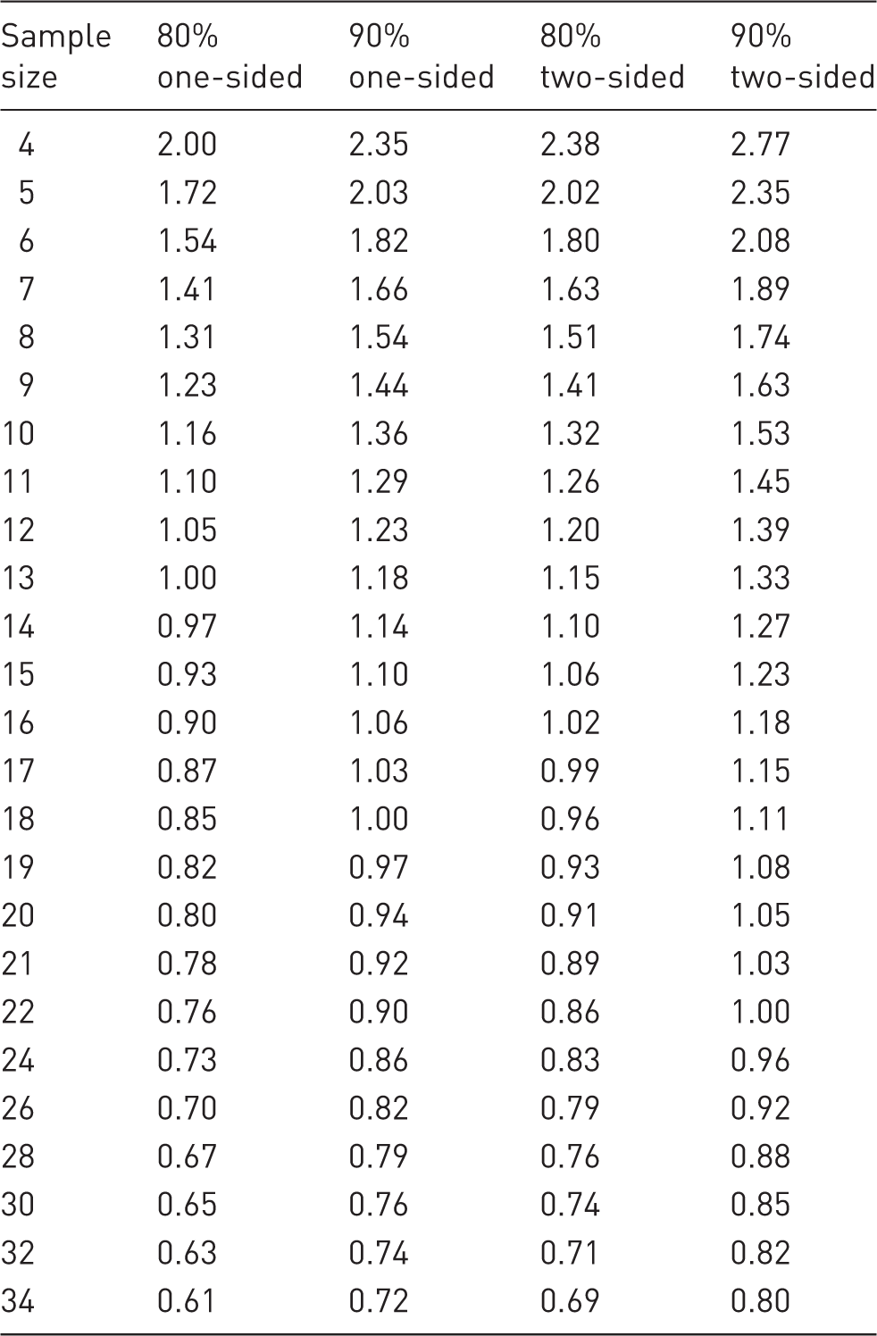
This note reviews the three methods of determining sample size (“tradition” or “common sense”, the “resource equation” and the “power analysis”) and shows that they are related. A scientist can make a provisional choice of a sample size using “common sense” or the resource equation. Then, using the mathematics of the power analysis, he or she can easily check the magnitude of the response likely to be detectable for a specified level of power, significance, and sidedness. All that is needed is an estimate of the standard deviation (SD), Table 1 and some simple arithmetic. Scientists can easily investigate the effect of changing the provisional sample size should they wish to do so.

Table 1.

Cohen’s d (SESs) for sample sizes of 4–34 subjects per group assuming 80% and 90% power, a 5% significance level and a one-sided or two-sided test.

Sample size	80% one-sided	90% one-sided	80% two-sided	90% two-sided
4	2.00	2.35	2.38	2.77
5	1.72	2.03	2.02	2.35
6	1.54	1.82	1.80	2.08
7	1.41	1.66	1.63	1.89
8	1.31	1.54	1.51	1.74
9	1.23	1.44	1.41	1.63
10	1.16	1.36	1.32	1.53
11	1.10	1.29	1.26	1.45
12	1.05	1.23	1.20	1.39
13	1.00	1.18	1.15	1.33
14	0.97	1.14	1.10	1.27
15	0.93	1.10	1.06	1.23
16	0.90	1.06	1.02	1.18
17	0.87	1.03	0.99	1.15
18	0.85	1.00	0.96	1.11
19	0.82	0.97	0.93	1.08
20	0.80	0.94	0.91	1.05
21	0.78	0.92	0.89	1.03
22	0.76	0.90	0.86	1.00
24	0.73	0.86	0.83	0.96
26	0.70	0.82	0.79	0.92
28	0.67	0.79	0.76	0.88
30	0.65	0.76	0.74	0.85
32	0.63	0.74	0.71	0.82
34	0.61	0.72	0.69	0.80

Current methods of determining sample size

It is assumed that a proposed experiment has two groups, namely “control” and “treated”, and the dependent variable is, or can be made, suitable for statistical analysis using a t-test or an analysis of variance. The determination of sample size for discrete data is not discussed here.

It is also assumed that the aim is to design an experiment which is both small and powerful.

1. “Tradition” or “common sense”

Currently, most investigators choose sample sizes which were used, apparently successfully, by other investigators conducting similar work. Given the wide range of types of experiment, independent and dependent variables, experimental units, species, strains and outcome variables in laboratory animal research, this seems to be a sensible approach. Cox and Reid¹¹ state that “Except in rare instances_…, a decision on the size of the experiment is bound to be largely a matter of judgement and some of the more formal approaches to determining the size of the experiment have spurious precision”. They are probably referring to the “power analysis”. Sir David Cox is the author of two books on experimental design^11,12 and is the first winner of the “International Statistics Prize”, so his views should be taken seriously.

2. “The resource equation”

This method¹³ is based on previous experience largely from agricultural and industrial research. The equation is:

\begin{matrix} E = (thetotalnumberofexperimentalunits) \\ - (thenumberoftreatmentgroups) \end{matrix}

E should be chosen to be between about 10 and 20, although these are not rigid limits.

This method recognises that there is a slight “sweet spot” within these two limits. If fewer animals were to be used than the lower limit, then the chance of a type II error (false-negative result) increases substantially. If more animals were to be used than the upper limit, then the cost and use of animals will increase for only a modest gain. The method also shows that if there are more than two treatments, the number of experimental subjects per treatment can be reduced. The method is a useful addition to “common sense”. But funding organisations and ethical review committees are increasingly demanding the use of a power analysis to determine sample size. Apparently they are under the (false) impression that it provides an objective method of determining sample size.

3. “Power analysis”

Introduced by Jacob Cohen in in the 1960s,¹⁴ this method depends on a mathematical relationship between six variables. If five of these are specified, the sixth one (usually sample size) can be estimated, using dedicated software.

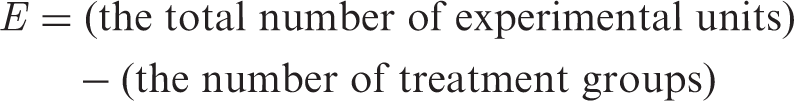
The six variables and some of the factors which influence them are shown in Figure 1.

1. The SD

Figure 1.

The six factors directly used in a power analysis (labelled 1–6), and factors which may influence them. Usually a power analysis is used to determine sample size (6) for specified levels of the other five variables. However, here the aim is to determine the effect size (2), for a given sample size, for reasons which are explained in the text.

An estimate of the SD of the character of interest should be obtained from previous experiments involving animals of the same species, strain, age, gender and health status as the animals which are to be used. If it is not available a pilot study using small numbers of untreated animals of the same strain etc. will be needed.

Powerful small experiments require tight control of the inter-individual variation. This depends on several factors, shown in Figure 1. The animals (or other experimental subjects) should be as uniform as possible. Within-subject and randomised block designs¹⁵ are likely to give better control of variation than between-subject designs.¹⁶ Variation will be minimised if the experimental animals are free of clinical or sub-clinical infection and have been raised in a good environment. They should be of uniform age and weight. Genetic variation can be controlled by using inbred or F1 hybrid strains of mice and rats.¹⁷

Measurement error needs to be minimised. Duplicate or repeat determinations of the outcome variable can sometimes be used to reduce such variation.¹⁸ The experimental data need to be of high quality and collected using “Good Laboratory Practice” standards, and staff should be well trained in husbandry and the collection of the data.

2. The effect size (ES)

This is the difference between the means of the two groups which are being compared. Large ESs are easier to detect than small ones. So, when planning an experiment the aim should be to give as high a dose (or equivalent) as possible, but not so high as to cause unwanted side effects.

Where possible choose sensitive strains and species of animals, or avoid insensitive ones. For example, Sprague-Dawley rats from one commercial supplier are not suitable for studies of the endocrine disruptor bisphenol A as they are insensitive to steroid substances.¹⁹ Some variables are more sensitive than others, so more sensitive ones should be chosen where possible.

3. The power

This is the probability that the experiment will reject the null hypothesis when it is false. A power of 80% or 90% is usually specified. For any given sample size there is a complete range of levels of power and an associated ES that the experiment is likely to be able to detect. This is explained in more detail below.

Note that if a completed experiment has rejected the null hypothesis it was clearly powerful (although it could be a false-positive result). However, the converse is not true. If an experiment fails to reject the null hypothesis it could be either because it lacked power or because there was no treatment effect of sufficient size to be worth trying to detect. In a power analysis the aim is only to design experiments to be able to detect ESs which are sufficiently large to be of scientific interest.

4. The significance level

This is the probability that the experiment will produce a false-positive result (a type I or α error). It is usually set at p = 0.05. So in a well-designed and unbiased experiment there is a 5% chance of making a type I (false-positive) error. Occasionally a case can be made for using a different level. But specifying a 1% significance level, for example, would increase the required sample size or decrease the power.

5. The sidedness of the test

A two-sided test, in which the mean of the treated group could be either larger or smaller than the mean of the control group, is usually used. But if the response can only go, or would only be of interest, in one direction then a one-sided test should be used. A one-sided test leads to a more powerful experiment or requires a smaller sample size.

6. The sample size

This is the number of experimental subjects in each group. Usually, a power analysis is used to estimate a suitable sample size for a proposed experiment. However, the alternative, used here, is for the investigator first to choose a sample size based on “common sense”, previous studies and/or the “resource equation” and then calculate the ES likely to be detectable using the mathematics of a power analysis, as incorporated in Table 1. This is explained below. This approach is easy to understand and is less prone to error than the more conventional approach.

The “standardised effect size” (SES or Cohen’s d)

The SES or Cohen’s d is a useful statistic. It is the ES divided by the pooled SD (SD_pooled). So it is the magnitude of the difference between the means of two groups in units of SDs. The SES is widely used when combing the results of several studies in a meta-analysis.²⁰ It can also be used when comparing the treatment response for different variables because they are all expressed in the same units (SDs). In toxicity tests, for example, measurements of haematology, clinical biochemistry, organ weights and other factors can be combined to give an over-all response to a test chemical in SD units.²¹ Moreover, the SES is directly related to sample size if the power, sidedness and significance level in a proposed experiment are fixed.

Based on human studies Cohen (who was a psychologist) suggested that responses to a treatment resulting in SESs of 0.2, 0.5 and 0.8 SDs would represent small, moderate and large treatment responses requiring sample sizes of 394, 64, or 26 subjects per group, respectively, to detect the effect. This is assuming an 80% power, a 5% significance level and a two-sided t-test.

However, laboratory animals are intrinsically much more uniform than humans, so the SDs are lower. Groups of animals can be obtained of similar age and weight, free of clinical or sub-clinical infection, fed the same diet and housed in the same environment. Inbred strains of mice and rats can also be used in which all animals are genetically identical. All these factors lead to lower SDs. Higher responses may also be obtained. Higher dose levels of test substances can be given and sensitive species and strains can often be chosen or insensitive ones avoided.

As a result, much higher SESs are observed in laboratory animal experiments than in clinical trials. Here it is suggested that SES of 1.1 “extra-large”, 1.5 “gigantic” and 2.0 SDs “awesome” are added to take account of laboratory animal experiments, including in vitro studies using animal cells or extracts. Detecting SES of these magnitudes would require sample sizes of 17, 8, and 5 subjects per group, respectively, with an 80% power, a 5% significance level and a two-sided t-test.

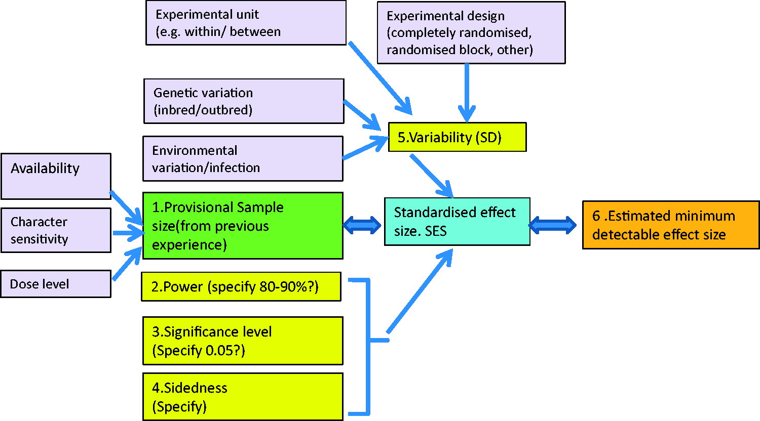
Figure 2 (a)–(d) shows the estimated SESs from an experiment on the effect of chloramphenicol on four haematological outcomes in mice of four inbred strains and one outbred stock at six dose levels. The raw data for these figures is included in the original publication.²² There are clear dose-related differences in response. Many SESs are “gigantic”, or “awesome”, being well over two SDs. There are clear strain differences in sensitivity. For example, the outbred CD-1 stock was relatively more resistant to chloramphenicol for all four characters than the four inbred strains, and the white blood cell count (WBC) response to chloramphenicol in strain C3H was much higher than in other strains.

Figure 2.

Observed standardised effect sizes (SES) for four haematological parameters in mice treated with chloramphenicol at six dose levels (mg/kg). Note important strain and dose level effects.

It is not necessary to know how to calculate the SESs when using them in estimating sample size as discussed below. But investigators are encouraged to quote the observed SESs from their completed experiments. Details are given in the Appendix.

The relationship between the SESs and sample size.

Figure 3 shows the relationship between sample size and SESs, over the range of 4–34 animals (or other experimental units) per group for a significance level of 0.05 and a two-sided test, for power levels of 60%–90%.

Figure 3.

Standardised effect size (SES or Cohen’s d) as a function of sample size (per group) for four levels of power (60%–90%) assuming a two-sided t-test with a 5% significance level and a quantitative dependent variable. The vertical dotted lines show the range of sample sizes using the “resource equation” method of determining sample size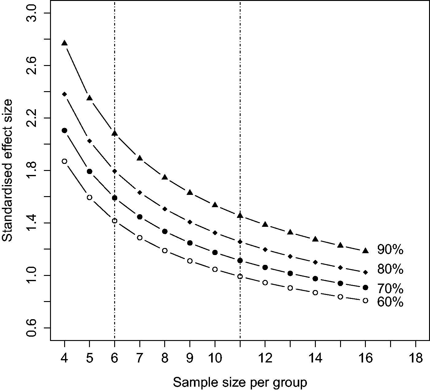

Note that for any given sample size there is a range of SESs and power levels likely to be detectable. For example, with six animals per group there will be a 90% chance of detecting an SES of about 2.1 SDs, an 80% chance of detecting an SES of 1.8 SDs, a 70% chance of detecting an SES of 1.6 SDs and a 60% chance of detecting an SES of 1.4 SDs and so on down to a 5% chance of detecting a non-existent response (a type I error). As a consequence, an investigator will sometimes be “lucky” and detect an effect which is smaller than the experiment was designed to be able to detect. Anyone wanting to repeat an experiment should use a larger sample size than was used in the original experiment.

Table 1 gives the corresponding SES for sample sizes ranging from 4–34 subjects per group for 80% and 90% power and a 5% significance level, one sided or two sided. A more extensive table is given by Ellis.²⁰

The “Keep It Simple, Stupid” (KISS) approach to the determination of sample size

Most investigators base sample sizes on past experiments which appear to have given satisfactory results. Given the wide range of variables shown in Figure 1, this makes sense.¹¹ However, funding organisations and ethical review committees often require scientists to justify their sample sizes using a power analysis.

The KISS approach combines these two methods. Scientists make a provisional estimate of the sample size using “common sense” and/or the resource equation, then use a table and some simple arithmetic to estimate the ES that the experiment is likely to be able to detect for a given power, etc. Optionally, they may express this ES as a percentage change. If, on reflection, they want to be able to detect a smaller ES they can increase the provisional sample size and re-do the calculations. They can then legitimately explain their choice in terms of the power analysis.

The procedure is as follows:

1. Plan the experiment.

Specify the purpose of the experiment and consider whether comparable results could be obtained from using methods which do not involve live animals.

Assuming that the use of animals is essential, specify the species, strain, age/weight and gender of the animals to be used. Identify the “experimental unit” (this is the unit of randomisation and of statistical analysis. Any two experimental units must be able to receive different treatments). Specify treatments (doses, methods of administration), number of treatment groups, outcome variables to be measured, timeline, and experimental design (e.g. completely randomised, randomised block, factorial, other).

2. From previous studies, obtain one or more estimates of the mean and SD of the variable of interest in control subjects. It may be best to choose a high and a low SD.

3. Choose a provisional sample size based on previous studies, the literature, the resource equation and “common sense”.

4. Find the SES for the provisional sample size in Table 1, with the desired power level and sidedness of the test. Multiply the SES by the SD to give the “predicted detectable ES” for the chosen levels of power, etc. This can be expressed as a percentage change if it would make it easier to understand.

5. Decide whether the “predicted detectable ES” is acceptable (i.e. whether it will detect a sufficiently small effect, should it be present). If not then choose a larger provisional sample size and re-do the calculations.

6. In the Materials and methods section of the resulting publication, and in accordance with the Animal Research: Reporting of In Vivo Experiments (ARRIVE) guidelines,²³ a statement such as the following could be included:

“A power analysis shows that the sample size of XX has a XX% power to detect an effect size of XX (units or %) assuming a 5% significance level and an XX-sided test.”

Where the XXs are replaced by the appropriate values.

In order to avoid publication bias, the results of the experiment should be written up and submitted for publication whether or not the observed differences were “statistically significant”. Negative results are of extra value when backed up by a power analysis as shown because they help to preclude a large undetected effect.

Example 1

Question: “Does a potential new drug alter red blood cell (RBC) count in mice?”

From a published study, C57BL/6 female mice had a mean RBC count of 9.19 with an SD of ±0.70 (n/µl). (Make sure that it is the SD not the SEM.)

Suppose a provisional sample size of n = 12 mice/group is chosen, based on previous studies.

From Table 1 for a sample size of 12 with a 90% power and a two-sided test, SES = 1.39.

Therefore the “predicted detectable ES” (SES*SD) is 1.39 × 0.70 = 0.97 (n/µl).

Or as a percentage = (0.97/9.19) × 100 = 11%.

Assuming that this “predicted detectable ES” is judged to be acceptable, a sample size of 12 mice per group can be used.

Following the ARRIVE guidelines,²⁴ a statement such as the following should be written in the Materials and methods section

“A power analysis shows that the sample size of 12 mice/group has a 90% power to detect an ES of 0.97 n/µl or an 11% change, assuming a 5% significance level and a two-sided test.”

Example 2

An investigator plans to study the effect of a drug on chosen haematological and biochemical characters in Sprague-Dawley rats. Means and SDs are taken from a published paper.²⁵ A sample size of 12 rats per group is proposed.

The calculations are shown in Table 2. Quite small changes of the order of 4% to 5% in RBC and haemoglobin (HGB) are likely to be detectable, but only large changes will be detectable in WBCs and clinical biochemistry. Note that the power analysis does not predict the actual magnitude of the response, only how large the response would need to be to be detectable. So, for example, if the ES as a percentage of the mean for WBC is 36% or greater, then it will probably be detected assuming the SDs are about the same as those published in the original paper.

Table 2.

Estimated detectable effect size (ES) and % change in some haematological and clinical biochemistry characters in outbred Sprague-Dawley rats assuming two treatment groups (“Treated” and “Control”) for sample size N = 12 (SES = 1.39, Table 1).

Biomarker	Units	Sex	Mean	SD	Estimated detectable ES^a in SDs	Estimated % change
RBC	(10⁶/ll)	Male	8.61	0.27	0.38	4
HGB	(g/dl)	Male	15.80	0.40	0.56	4
WBC	(10³/ll)	Male	9.71	2.50	3.48	36
RBC	(×10⁶/ll)	Female	8.29	0.32	0.44	5
HGB	(g/dl)	Female	15.70	0.60	0.83	5
WBC	(10³/ll)	Female	5.69	1.48	2.06	36
AST	(U/l)	Male	105.00	23.00	31.97	31
ALT	(U/l)	Male	36.00	8.00	11.12	31
SDH	(U/l)	Male	7.30	4.60	6.39	88
AST	(U/l)	Female	117.00	33.00	45.87	39
ALT	(U/l)	Female	42.00	18.00	25.02	60
SDH	(U/l)	Female	13.20	5.50	7.65	58

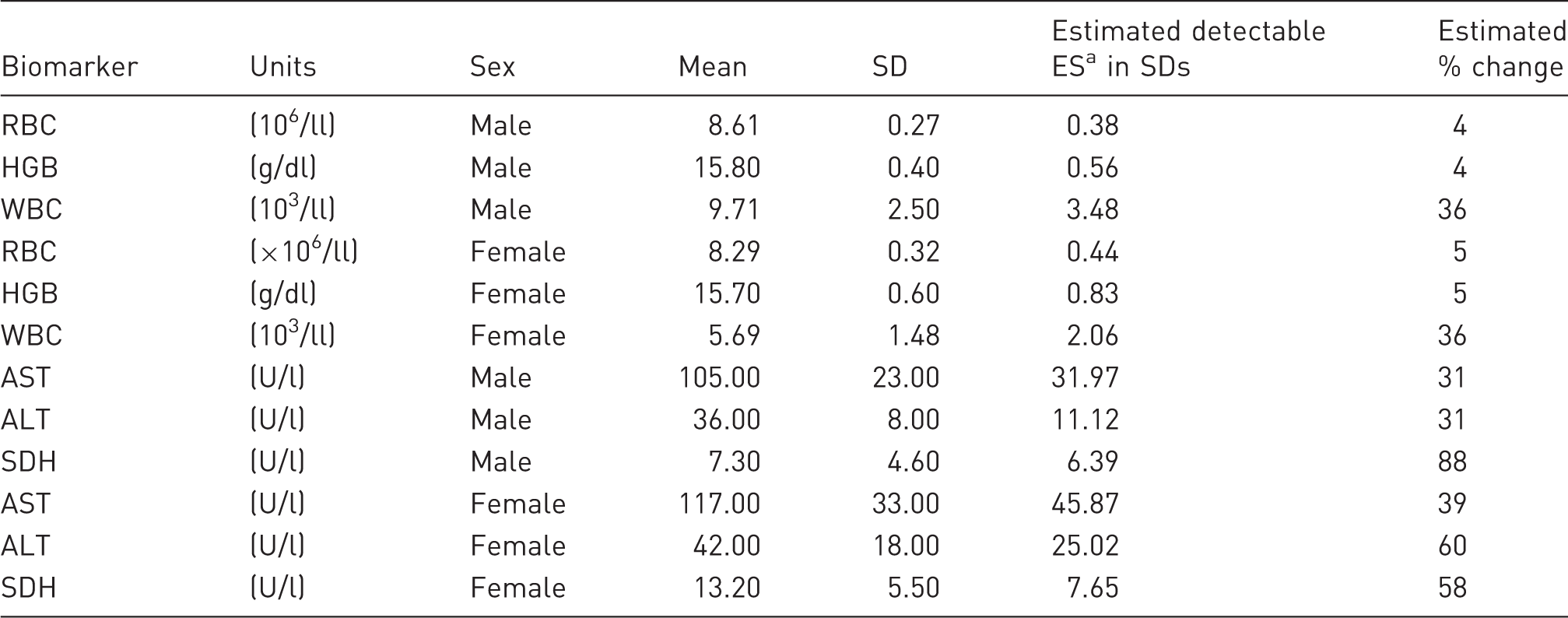
This assumes a 90% power a 5% significance level and a two-sided test. It is the SD × SES (1.39 for a sample size of 12 in Table 1).

RBC: red blood cell count; HGB: haemoglobin; WBC: white blood cell count; AST: aspartate aminotransferase; ALT: alanine aminotransferase; SDH: sorbitol dehydrogenase; SES: standardised effect size.

Having performed the calculations, the investigator has still to decide whether the sample size is appropriate.

More than two groups

The KISS method estimates the ES that a comparison between any two groups is likely to be able to detect for the specified sample size, power, significance level and sidedness of the test. If another group (say an intermediate dose or a qualitatively different treatment) of the same size is added then the same calculations apply to it. However, with more than two groups there will be a better estimate of the SD so sample size can be slightly reduced. The resource equation method should give some guidance on this, but the dangers of “spurious precision” and the importance of “common sense” should not be forgotten.

If an additional factor such as gender is added in a factorial design so that there are four groups (male and female control and treated), then sample size is the number of males plus females in the treated and control group.

Formal power analysis is available for experiments with several treatment groups, but it is subject to even more “spurious precision” than if just two groups are involved.

Discussion

No one method of determining sample size is entirely satisfactory. “Common sense” may work well with an experienced investigator who is thoroughly familiar with his or her material and has already performed a number of experiments similar to the one proposed. But it is less satisfactory for those starting a new research topic. The resource equation method provides a useful rule of thumb method for avoiding experiments which are probably either too small, so likely to lead to false-negative results, or unnecessarily large leading to a waste of resources. But it doesn’t have the (possibly spurious) mathematical justification of the power analysis.

The power analysis is complex and it involves a subjective element because the investigator must decide the minimum ES likely to be of scientific interest. It also suffers from spurious precision because there are several important variables, such as the sensitivity of the chosen experimental material, which are not taken into account. Normally, it also requires access to specialised software which, although readily available, requires an additional level of understanding. If scientists are required to use unfamiliar software and unfamiliar variables, there is a danger that their calculations will be incorrect. The KISS approach of choosing sample size using “common sense”, and/ or the resource equation and combining it with the power analysis provides a simplified solution to the problem of determining sample size in laboratory animal experiments.

Footnotes

Declaration of Conflicting Interests

The author(s) declared no potential conflicts of interest with respect to the research, authorship, and/or publication of this article.

Funding

The author(s) received no financial support for the research, authorship, and/or publication of this article.

Appendix

References

Begley

Ellis

. Drug development: Raise standards for preclinical cancer research. Nature 2012; 483: 531–533.

Scott

Kranz

Cole

et al.

Design, power, and interpretation of studies in the standard murine model of ALS. Amyotroph Lateral Scler 2008; 9: 4–15.

Prinz

Schlange

Asadullah

. Believe it or not: How much can we rely on published data on potential drug targets? Nat Rev Drug Discov 2011; 10: 712–712.

Freedman

Cockburn

Simcoe

. The Economics of reproducibility in preclinical research. PLoS Biol 2015; 13: e1002165–e1002165.

Festing

. We should be designing better experiments. Vet Anaesth Analg 2003; 30: 59–61.

Festing

. Principles: The need for better experimental design. Trends Pharmacol Sci 2003; 24: 341–345.

Festing

MFW

. The scope for improving the design of laboratory animal experiments. Lab Anim 1992; 26: 256–267.

Kilkenny

Parsons

Kadyszewski

et al.

Survey of the quality of experimental design, statistical analysis and reporting of research using animals. PLoS One 2009; 4: e7824–e7824.

Bebarta

Luyten

Heard

. Emergency medicine animal research: Does use of randomization and blinding affect the results? Acad Emerg Med 2003; 10: 684–687.

10.

Button

Ioannidis

Mokrysz

et al.

Power failure: Why small sample size undermines the reliability of neuroscience. Nat Rev Neurosci 2013; 14: 365–376.

11.

Cox

Reid

. The theory of the design of experiments, Boca Raton, FL: Chapman and Hall/CRC Press, 2000.

12.

Cox

. Planning experiments, NY: John Wiley and Sons, 1958.

13.

Mead

. The design of experiments, Cambridge, NY: Cambridge University Press, 1988.

14.

Cohen

. Statistical power analysis for the behavioral sciences, Hillsdale NJ: Lawrence Erlbaum Associates, 1988.

15.

Festing

. Randomized block experimental designs can increase the power and reproducibility of laboratory animal experiments. ILAR J 2014; 55: 472–476.

16.

Festing

Overend

Cortina Borga

et al.

The design of animal experiments, 2nd ed. London, UK: Sage Publications, 2016.

17.

Festing

. Genetically defined strains in drug development and toxicity testing. Methods Mol Biol 2016; 1438: 1–17.

18.

Karp

Baker

Gerdin

et al.

Optimising experimental design for high-throughput phenotyping in mice: A case study. Mamm Genome 2010; 21: 467–476.

19.

Richter

Birnbaum

Farabollini

et al.

In vivo effects of bisphenol A in laboratory rodent studies. Reprod Toxicol 2007; 24: 199–224.

20.

Ellis

. The essential guide to effect sizes, Cambridge: Cambridge University Press, 2010.

21.

Festing

. Extending the statistical analysis and graphical presentation of toxicity test results using standardized effect sizes. Toxicol Pathol 2014; 42: 1238–1249.

22.

Festing

Diamanti

Turton

. Strain differences in haematological response to chloramphenicol succinate in mice: Implications for toxicological research. Food Chem Toxicol 2001; 39: 375–383.

23.

Kilkenny

Altman

. Improving bioscience research reporting: ARRIVE-ing at a solution. Lab Anim 2010; 44: 377–378.

24.

Kilkenny

Browne

Cuthill

et al.

Improving bioscience research reporting: The ARRIVE guidelines for reporting animal research. PLoS Biol 2010; 8: e1000412–e1000412.

25.

Delaney

Karaman

Roper

et al.

Thirteen week rodent feeding study with grain from molecular stacked trait lepidopteran and coleopteran protected (DP-ØØ4114–3) maize. Food Chem Toxicol 2013; 53: 417–427.

26.

Perron

Pack

Veasey

. Diet/Energy balance affect sleep and wakefulness independent of body weight. Sleep 2015; 38: 1893–1903.

On determining sample size in experiments involving laboratory animals

Abstract

Keywords

Introduction

Current methods of determining sample size

The “standardised effect size” (SES or Cohen’s d)

The relationship between the SESs and sample size.

The “Keep It Simple, Stupid” (KISS) approach to the determination of sample size

Example 1

Example 2

More than two groups

Discussion

Footnotes

Declaration of Conflicting Interests

Funding

Appendix

References