
Abstract
Electron tomography has emerged as the leading method for the study of three-dimensional (3D) ultrastructure in the 5–20-nm resolution range. It is ideally suited for studying cell organelles, subcellular assemblies and, in some cases, whole cells. Tomography occupies a place in 3D biological electron microscopy between the work now being done at near-atomic resolution on isolated macromolecules or 2D protein arrays and traditional serial-section reconstructions of whole cells and tissue specimens. Tomography complements serial-section reconstruction by providing higher resolution in the depth dimension, whereas serial-section reconstruction is better able to trace continuity over long distances throughout the depth of a cell. The two techniques can be combined with good results for favorable specimens. Tomography also complements 3D macromolecular studies by offering sufficient resolution to locate the macromolecular complexes in their cellular context. The technology has matured to the point at which application of electron tomography to specimens in plastic sections is routine, and new developments to overcome limitations due to beam exposure and specimen geometry promise to further improve its capabilities. In this review we give a brief description of the methodology and a summary of the new insights gained in a few representative applications. (
Keywords
T
Microscope improvements include computer control, improved specimen stages, high-sensitivity digital image recording, field-emission electron sources, and energy filtering. Combined with increased computational power and developments in image-processing software, two important applications of biological TEM for 3D structure determination have emerged. The first, and currently the major application, is high-resolution biological electron microscopy (reviewed by Stowell et al. 1998). This area includes electron crystallography (reviewed by Glaeser 1999; Subramaniam and Henderson 1999) for ordered arrays (i.e., so-called 2D crystals), helical reconstruction methods (reviewed by Stewart 1988; De Rosier et al. 1999) for helical filaments, and single-particle reconstruction methods (e.g., Frank and Agrawal 2000) for single macromolecules and macromolecular assemblies. The second application is electron tomography, the subject of this review. Tomography is especially useful for detailed studies of organelle-sized structures.
In the high-resolution applications, (e.g., 3D resolution better than 1 nm), TEM complements X-ray crystallography and nuclear magnetic resonance (NMR) studies. This was dramatically illustrated by the recent use of electron crystallography to determine the atomic structure of the tubulin dimer, a key cytoskeletal component involved in many cell processes (Nogales et al. 1998). To understand cellular function, however, we must go beyond determining the high-resolution structure of isolated components and place these components into their cellular context. Here TEM is the method of choice because it can be used to determine “structural maps” of more complex macromolecular assemblies with sufficient resolution (2–3 nm) that high-resolution structural determinations of component molecules can be “docked” (i.e., fitted) into the complete macromolecular complex (Baker and Johnson 1996; Wriggers et al. 1999). This approach has been successfully used to insert the atomic map of tubulin into the microtubule lattice (Nogales et al. 1999), to determine the atomic interactions between the myosin S1 fragment and F-actin in decorated actin filaments (Rayment et al. 1993), and to track myosin structural changes on the molecular level during the mechano–chemical cycle accompanying insect flight muscle contractions (Taylor et al. 1999).
As impressive as this docking approach has been, its application has thus far been limited to a small subset of cell structures. The reason for this is that high- and medium-resolution structural determination, whether by X-ray crystallography, NMR, or TEM, requires averaging thousands of copies of an “identical” motif (e.g., protein molecules in a 3D or 2D crystal lattice, subunits of a helix, or computationally aligned particles such as ribosomes). Because most organelles and cellular substructures are complex pleomorphic assemblies that show considerable individual variation, they cannot be averaged as identical motifs. Electron tomography is the only computational 3D reconstruction technique not based on averaging. Therefore, it is generally the method of choice for 3D reconstruction of subcellular structures. Although resolution is necessarily limited by the lack of averaging, 3D resolution of 5–10 nm is currently obtained. This enables tomography to bridge the gap between serial section reconstruction and the higher-resolution approaches (see below). The ultimate goal of electron tomography is to compute 3D structural maps of cell organelles with sufficient resolution to locate “molecular signatures” of individual macromolecules and thereby enable the docking approach to be extended to a much wider range of macromolecules and cell substructures.
Here we provide a general introduction to electron tomography, along with a summary of selected applications during the previous decade and a brief look into current developments.
General Approach of Electron Tomography
Background for 3D Imaging
Like all forms of imaging that use penetrating radiation, TEM provides a translucent or “X-ray” view of the specimen. Although this has the advantage of enabling the user to see inside the structure, it also has the disadvantage that structural details from different depths in the specimen are superimposed in a 2D projection. This process of image formation is illustrated in Figure 1A, in which a 2D “smiley face” is projected onto a 1D line. Peaks of mass are recorded in those segments of the line where the imaging rays transverse through an eye or the nose in addition to the mouth. Such images are confusing and counterintuitive, both because details are superimposed upon one another and because we are accustomed to viewing surfaces in the everyday world. That is why the surface views provided by scanning electron microscope images are easier to interpret than TEM images.
The traditional approach to circumvent the problem of superimposed features in the 2D images is to embed specimens in plastic and cut sections so thin (i.e., 40–80 nm thick) that each section is effectively a 2D slice from the specimen. When the pitfalls of structural interpretation from 2D information became apparent, methods were developed for 3D reconstruction via stacking serial thin sections (e.g., Sjöstrand 1958; Rieder 1981; Bron et al. 1990). Although labor-intensive, the development of computer methods for alignment and tracing has made serial section reconstruction reasonably efficient and effective (e.g., Kremer et al. 1996; Marko and Leith 1996). Nevertheless, this approach is limited by the fact that resolution in the depth dimension cannot exceed twice the section thickness (see McEwen and Marko 1999). Although there are reports that serial sections can be cut as thin as 10 nm (Mastronarde et al. 1997), this procedure is very demanding, and the utility of ultrathin serial sections for 3D reconstructions has yet to be demonstrated. Furthermore, even at 10-nm thickness, resolution in the depth dimension is still limited to 20 nm as opposed to 5–10 nm for electron tomography. An additional difficulty is the possibility of specimen distortion from compression during sectioning (Sjöstrand 1958; Hayat 2000).
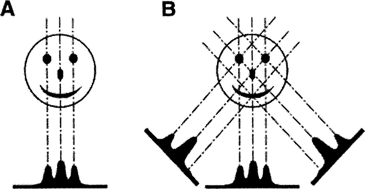
Illustration of projection imaging and reconstruction via back-projection. (
Electron tomography uses the opposite approach to solve the 2D projection problem. Plastic sections are cut thick enough (200–1000 nm) to contain a significant amount of information in the depth dimension. The superimposition of image detail is then resolved by computing a 3D reconstruction of individual thick sections, using back-projection algorithms that are essentially the same as those used in medical imaging procedures such as magnetic resonance imaging (MRI) and computerized axial tomography (CAT). Briefly, a projection image records the amount of mass density encountered by imaging rays, as illustrated in Figure 1A. Because the path of the imaging rays is known (or can be computed), the only unknown is how specimen mass was distributed along the imaging path (i.e., one dimension is always “lost” during projection imaging). The approach of the back-projection algorithms is to simply distribute the known specimen mass evenly over computed back-projection rays that in effect retrace the path of the imaging rays. In this way, specimen mass is projected back into a reconstruction volume (i.e., “back-projected”). When this process is repeated for a series of projection images recorded from different tilt angles, back-projection rays from the different images intersect and reinforce one another at the points where mass is found in the original structure, as illustrated in Figure 1B. Hence, the 3D mass of the specimen is reconstructed from a series of 2D images. For a more in-depth description of imaging and tomographic reconstruction, see Koster et al. (1997) and McEwen and Heagle (1997).
Data Collection
Data collection for electron tomography is accomplished by tilting the specimen in the electron beam. The resolution and quality of the reconstruction are directly dependent on how finely spaced the tilt images are and over how wide an angular range they extend. Therefore, the strategy is to collect as many tilt images over as wide an angular range as is feasible. Generally, this consists of collecting images at 1–2° angular intervals over an angular range of ± 60 to 70°. Therefore, electron tomography requires that the electron microscope be equipped with an accurate tilt stage and a specimen holder that can accommodate reasonably high tilt angles. Although it is possible to collect a tomographic tilt series on a manual tilt stage, such a procedure is extremely tedious. Therefore, routine application of tomography requires a motorized tilt stage that is reasonably eucentric, and is equipped with a digital angular readout. These features are readily available on most modern electron microscopes.
Another feature that is becoming increasingly common on electron microscopes is a digital camera for image recording. Because the data must be in digital form for computation of the reconstruction, direct digital recording can be a considerable timesaver compared with film recording and subsequent digitization. Direct digital recording also obviates the need to interrupt data collection for film changes and processing. Because it is now recommended to use dual-axis data collection whenever feasible (see below), typical electron tomographic data sets range from 120 to 280 images. Furthermore, one usually wants to see more than one example of the 3D structure and is often interested in different functional states of the organelle and/or examples from different cell types. Therefore, individual studies can easily involve collecting thousands of images and data throughput becomes an important consideration. In such situations, image acquisition via a CCD camera can be an important boon. For many studies, an image size of 1024 × 1024 pixels is sufficient to ensure the requisite pixel resolution over an adequate area of the specimen. However, for studying large areas of a cell, montaging (i.e., pasting together CCD images from adjacent slightly overlapping CCD images) may be needed. This function is normally supplied along with the imaging software purchased with the CCD camera system. For these large specimen areas it is often preferable to go back to using film because film provides greater spatial resolution (i.e., many more pixels) than CCD cameras (e.g., see Ladinsky et al. 1999).
Another important consideration for data collection is accelerating voltage. At 60° tilt, the path length of the electron beam through the specimen is twice the specimen thickness. At 70° it is three times the specimen thickness. Therefore, at conventional accelerating voltages image quality rapidly deteriorates at high tilt angles. For this reason, intermediate-voltage (200–400 kV, IVEM), high-voltage (∼1.0 MV, HVEM), or energy-filtered electron microscopes are highly recommended for specimens thicker than 120–150 nm. Although a few smaller specimens, such as negatively stained preparations of isolated chromatin fibers, have been successfully studied with electron tomography using conventional accelerating voltages, most applications, particularly those using thick plastic sections, have used IVEMs or HVEMs. If access to an IVEM or HVEM equipped with a proper tilt stage is a limitation, data can be collected at one of the three NIH Biotechnological Resources that are set up for electron tomography: at the University of Colorado at Boulder; at the University of California at San Diego; and at the Wadsworth Center in Albany, NY. In addition to having the proper microscope, tilt stage, and camera, the Resources also have appropriate software packages and experienced personnel who can assist the user.
Data Processing
Because goniometers in electron microscopes are not perfectly eucentric (although some of the newer stages come extremely close), a certain amount of specimen tracking and refocus is necessary during collection of a tomographic tilt series. As a result, images of a tilt series must be translationally and rotationally aligned to bring them into register for computation of the 3D reconstruction (i.e., for the back-projection rays to intersect at centers of mass as illustrated in Figure 1B, the tilt images must be properly aligned). Alignment is most commonly accomplished by placing colloidal gold particles on the surface of the plastic section before collecting the tilt set. The positions of a given set of gold markers on each tilt image are then used by alignment algorithms to calculate shift vectors and rotations that bring the images into register (Lawrence 1992; Penczek et al. 1995; Mastronarde 1997). These algorithms also correct for the small magnification changes that accompany refocusing. The positions of gold particles in each tilt image are usually entered manually by an operator, although prototype marker-picking programs have been developed (Fung et al. 1996; Mastronarde 1997).
Once the tilt images are aligned, the 3D reconstruction can be computed using a back-projection algorithm. Although this is the most sophisticated and computer-intensive part of the process, it is also the part that is most transparent to the user. In general, one simply submits a program command file with the aligned images and waits for the reconstruction.
Visualizing the Reconstruction
After the 3D reconstruction is computed, the user is again faced with viewing a 3D object on a 2D medium such as the computer monitor. Often an experienced user can answer the biological questions at hand simply by viewing sequential thin 2D slices through the reconstructed volume. Although this is analogous to serial-section analysis, in tomography the thickness of the slices is determined by the pixel size chosen during digitization, and it can be as thin as 1 nm. Although viewing sequential slices frequently suffices for understanding simpler systems, 3D visualization is usually required for analysis of more complex organelles, communication of results to others, and quantitative measurements. The most common approach is to use some form of segmentation to extract features of interest from the volume and then to view the sub-volume using surface- or volume-rendering methods (reviewed by McEwen and Marko 1999). In brief, segmentation generally requires the user to manually trace the features of interest to isolate them from the rest of the reconstruction volume. Because contours must be entered manually, this step is typically the most time-consuming “bottleneck” in electron tomography. Once the reconstruction volume is segmented, a variety of modern graphics tools can be used to construct a 3D display of the selected components.
Figure 2 shows an example of volume segmentation applied to mitochondria. Membranes of individual cristae were traced using Sterecon, a software package developed in our laboratory for tracing 2D and 3D contours on serial sections and in 3D volumes (Marko and Leith 1996). In the example, contours were traced in 2D on successive slices of the tomographic reconstruction. The contours were then stacked, filled, and displayed as wire-frame and solid surfaces (see McEwen and Marko 1999). The color coding is used to distinguish individual cristae and the inner and outer membranes (see below; and Mannella et al. 1997). Analogous tools for segmentation, volume rendering, and visualization have been developed at the Boulder and San Diego Biotechnological Resources (Kremer et al. 1996; Perkins et al. 1997b).
Figure 3 illustrates the segmentation procedure being used to measure microtubule penetration into kinetochores from mammalian chromosomes. These data were collected to test a model predicting that the direction of kinetochore motion would be correlated with the depth of microtubule penetration into the outer plate (see McEwen and Heagle 1997). The direction of chromosome motion was determined via video light microscopy of chromosome motion up to the moment of rapid fixation. Correlative light and electron microscopy was then used to follow the chromosome through specimen preparation so that the pair of kinetochores from the video-tracked chromosome could be reconstructed via electron tomography. An edge-enhancing high-pass filter and a median smoothing filter were used to assist in tracing the boundaries of the microtubule and kinetochore outer plate respectively (Figures 3B and 3C). Penetration of the microtubule relative to the distal and proximal boundaries of the outer plate was measured from the tracings, as illustrated in Figure 3D, and penetration values from different slices of the 3D reconstruction were averaged to give a single value for the microtubule.
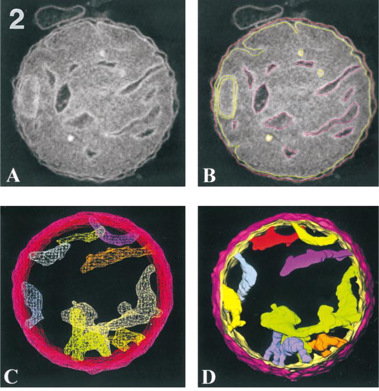
Visualization of a tomographic reconstruction from an isolated, plastic-embedded rat liver mitochondrion. The section thickness of the specimen is 0.5 μm, and the mitochondrion diameter is 1.5 μm. The tomographic reconstruction was computed from a dual-axis tilt series consisting of 140 images. (
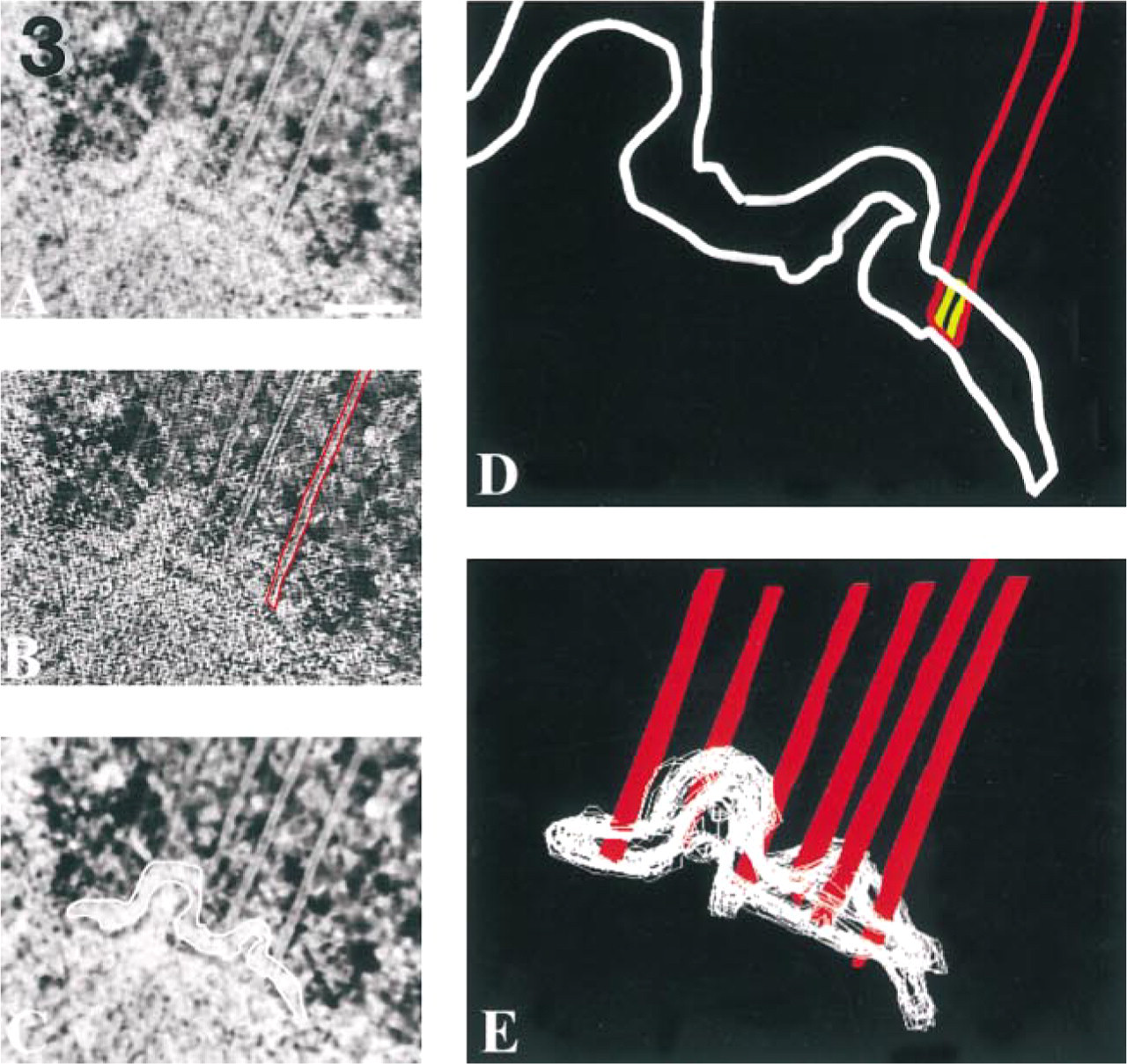
Tracing microtubules and the kinetochore outer plate in a single slice of a tomographic reconstruction. (
Limitations and Special Considerations
Limited Tilt Range
Because the planar dimensions of a standard TEM specimen grid are three orders of magnitude larger than its thickness, the effective electron beam path through the specimen rapidly increases for tilt angles above 60° (see illustration in McEwen and Marko 1999). As a result, it is usually not feasible to get good-quality images from plastic sections at tilt angles above 60–70°. Therefore, most tomographic tilt series have a wedge of missing data corresponding to the angular range between the maximal tilt angle collected and 90°. This limitation, which is not present in medical tomography, causes a distortion in the reconstruction known as the elongation factor (Frank and Radermacher 1986). The missing wedge also causes resolution in the 3D reconstruction to vary with viewing direction, which has the important consequence that linear elements, such as microtubules, membranes, and filaments, tend to fade from view when they are oriented perpendicular to the tilt axis (Penczek et al. 1995; Mastronarde 1997). This difficulty can be partially mitigated by rotating the specimen by 90° and collecting a second data set. This dual-axis data collection scheme reduces the missing angular range to a pyramid rather than a wedge (see illustration in McEwen and Marko 1999). This, in turn, reduces the elongation factor, produces resolution that is more isotropic, and reduces the tendency of linear elements to fade in certain viewing directions (Penczek et al. 1995; Mastronarde 1997).
Specimen Thinning
Another limitation is due to a 25–50% thinning of plastic sections that occurs on exposure to the electron beam (Luther 1992). The majority of this thinning occurs rapidly, during the time it takes to locate the desired area for tomography. This phenomenon becomes important only when one tries to find 3D information within a single plastic section (i.e., it is important for tomography but not for serial-section reconstruction). Because changes in section thickness during data collection complicate computation of the 3D reconstruction, the usual strategy is to pre-expose the specimen to allow completion of the initial rapid thinning phase. Then the tilt series is collected with as little additional electron dose as possible to avoid buckling of the section or further thinning during data collection. Although some investigators advocate stretching the reconstruction to compensate for section thinning, there is controversy as to whether thinning occurs via uniform shrinkage or surface collapse, and both processes probably contribute to the phenomenon (Bennett 1974; van Marle et al. 1995; Deng et al. 1999). In any case, section thinning and the missing angular range both degrade resolution in the depth dimension (i.e., the direction of the electron beam in the untilted view), and that loss is currently the limiting factor in obtaining higher 3D resolution from plastic-section electron tomography.
Resolution and Choosing Between Electron Tomography and Serial Section 3D Reconstruction
The resolution of a tomographic reconstruction is dependent upon the size of the specimen and the number of tilt views collected (Crowther et al. 1970). As may be intuitively evident from Figure 1, the more finely spaced the tilt views are collected, the more precise the 3D reconstruction of the specimen will be. For this reason, tomographic tilt series are usually collected in 1–2° angular intervals. In principle, the tilt angle interval could be made as small as one desires, but file handling considerations and limits to the accuracy of alignment schemes and electron microscope tilt stages have thus far made the extra data collection not worth the effort. However, with rapidly increasing computing power and recent technical advances in tilt stages, image processing, and data handling, it may soon become practical to collect tomographic tilt series at angular intervals of 0.5° or finer. Although this would potentially yield a two- to fourfold increase in resolution over current tomographic reconstruction schemes, other specimen-dependent limitations, such as focus gradients in high-tilt images, are likely to limit resolution to the 3–4-nm range for most plastic-embedded specimens.
For plastic sections, the nominal resolution for a given tilt angle interval is dependent on the section thickness and maximal tilt angle rather than the actual size of the reconstructed specimen (Radermacher 1992). Resolution can be quickly calculated from the simple formulation given by McEwen and Marko (1999):
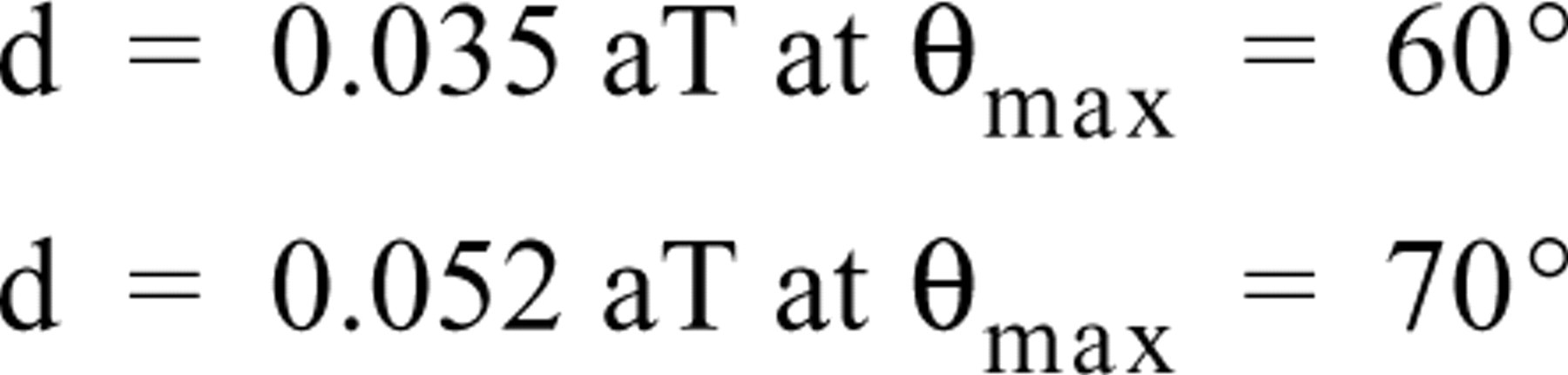
where d is resolution, a the angular interval (in degrees), T the section thickness, and θmax the maximal tilt angle in the series. Using this formulation, the resolution for a tomographic reconstruction of a specimen from a 0.250-μm-thick section is 8.7 nm if the tilt angle interval is 1° and the maximal tilt angle is 60°.
As mentioned above, the resolution is not isotropic. The above formula gives the resolution in planes perpendicular to the electron beam, represented in a tomographic reconstruction by slices parallel to the surface of the section. Resolution in planes (slices) perpendicular to the section surface is more strongly influenced by the elongation factor resulting from missing angular information. This factor decreases the resolution in the vertical (depth) direction in these slices by at least 20%. In the case of single-axis tilting, resolution in slices perpendicular to the tilt axis is further decreased by streaking artifacts that cause linear elements to disappear from view. These artifacts are barely noticeable, however, if the dual-axis tilting method is used (Penczek et al. 1995; Mastronarde 1997).
The easiest way to improve resolution is to cut thinner sections, as long as the section is thick enough to provide useful depth information in the 3D reconstruction. Previously, we emphasized that resolution limit is not synonymous with detection limit (McEwen and Marko 1999). As in light microscopy, features smaller than the theoretical resolution limit are frequently detected if they have sufficient contrast. Examples include fine details of initial crystal formation in normally mineralizing tissue (Landis et al. 1993), particles between mitochondrial inner and outer membranes (Mannella et al. 1997), and the topology of selectively stained Golgi and neural axons (Ellisman et al. 1990, Wilson et al. 1992; Ladinsky et al. 1994).
The resolution of serial-section reconstructions is limited to twice the section thickness (see McEwen and Marko 1999). Because serial sections are usually not cut thinner than 40–50 nm, resolution in the depth dimension is limited to 80–100 nm. However, resolution in the plane of the section is as high as the specimen preparation and imaging conditions permit (usually about 2 nm). As a result, thin fibrous elements can be traced over several micrometers if the fibers are oriented to present a cross-sectional view in the serial sections. This effectively places the low-resolution direction along the fiber axis, where resolution limitation is less critical. McDonald et al. (1992) used such a strategy to trace the microtubules in the mitotic spindles of PtK cells.
There are many applications for which serial-section analysis is adequate or even preferable to tomographic reconstruction. Hence, it is advisable to consider both approaches in the context of the goals of the study. Taking an example from our own work, it is easier to study the structure of an entire kinetochore using serial-section analysis because it is difficult to ensure that the whole structure will be contained within a single thick section. If the section is cut thick enough (several times thicker than the kinetochore) to ensure that the entire structure is contained, the tomographic resolution would be inadequate. Therefore, when we wanted to find out how many microtubules were bound to kinetochores under different conditions, we used serial-section analysis to ensure that we did not miss part of the kinetochore (McEwen et al. 1997). However, when we wanted to find out how far individual microtubules penetrated into the kinetochore we had to use electron tomography to get sufficient resolving power in 3D (Figure 3; McEwen and Heagle 1997). In the latter study it was not necessary to reconstruct the whole kinetochore.
Because tomography provides higher depth resolution and serial-section reconstruction is able to track complete structures over relatively large distances, it is natural to try to combine the two techniques. Serialsection tomography is in fact feasible (Soto et al. 1994), although it suffers from a 15–25-nm gap of missing material between the serial thick sections (Ladinsky et al. 1999). For the Golgi apparatus, this is not a serious problem because vesicles and membrane stacks are large enough to trace across the gap (Ladinsky et al. 1999). For the kinetochore, we find the problem more serious because there are no large landmark features to aid in aligning successive reconstructions, and many of the features we wish to track are too fine to trace across the gap (unpublished data). Therefore, the questions being asked will dictate whether tomography, serial-section reconstruction, or a combination of both is the most effective strategy to employ for a given study.
Examples of Recent Applications
The number of structural determinations employing electron tomography has grown rapidly over the past decade. A representative (but not exhaustive) list of electron tomographic applications is presented in Table 1. In the following paragraphs we describe five of these applications in more depth, with the intent of providing an indication of the scope of electron tomography and the kinds of questions that can be answered using this technique.
The key step in bone formation is deposition of calcium phosphate crystals into an extracellular matrix composed chiefly of Type I collagen. Electron tomography of initial crystal growth provided the first direct 3D imaging of the size, shape, orientation, and growth of crystals in normal mineralizing tissue (Landis et al. 1993). This visual evidence confirmed that the crystals were platelets rather than needles and that crystal length could extend beyond a single periodicity along the collagen fiber, demonstrating that growth was not restricted to a single “hole zone.” In addition, tomography demonstrated for the first time that although the platelet thickness was uniform, width was extremely irregular and variable. The patchwork appearance of the platelets strongly suggested that crystal growth could occur via the co-planar fusion of smaller platelets. These observations have important implications for the mechanism of early mineralization.
Tomographic 3D reconstructions of cells and cellular substructures a
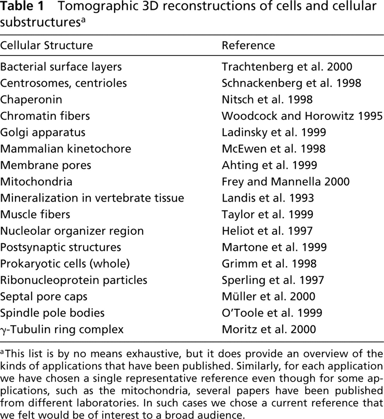
aThis list is by no means exhaustive, but it does provide an overview of the kinds of applications that have been published. Similarly, for each application we have chosen a single representative reference even though for some applications, such as the mitochondria, several papers have been published from different laboratories. In such cases we chose a current reference that we felt would be of interest to a broad audience.
An early controversy developed as to the structure of mitochondrial inner membrane folds known as cristae (reviewed in Mannella et al. 1997). One position held that cristae were tubular, with restricted access to the porous outer membrane and thereby to the cytosol, while the opposing view held that cristae were flat lamellar baffles with unrestricted access to the outer membrane and cytosol. This issue is important for bioenergetic calculations of the magnitude of pH gradients created by oxidative phosphorylation, because restricted access would enable generation of much larger chemiosmotic gradients than would free diffusion to the cytosol (Mannella 2000). Although the baffle model gained consensus and was incorporated into textbooks, there were several indications that cristae might also have a tubular character. Electron tomography revealed that cristae are pleiomorphic structures, sometimes flat and lamella-like and sometimes tubular. In both cases, however, they are connected to the intramembrane space by narrow (∼30 nm) tubular connections (Mannella et al. 1997; Perkins et al. 1997a; Frey and Mannella 2000; Nicastro et al. 2000). Although the proportion of tubular to lamellar cristae morphology appears to vary with the source and physiological state of the mitochondrion, connections to the cytosol remain restricted to narrow tubular openings. These results strongly argue for the restricted access model and hence require revision of accepted models for the structure and function of mitochondria.
The 3D reconstruction of a Golgi apparatus by Ladinsky et al. (1999) was one of the more ambitious electron tomography projects yet attempted. Serial thick-section electron tomography was used to reconstruct a 1 × 1 × 4-μm area of Golgi prepared using rapid freezing/freeze substitution (see below). Although molecular trafficking through the Golgi had been previously studied by a number of techniques, tomography revealed several previously unobserved features, such as extensive fenestration, many tubular extensions, and vesicle budding from the sides of all Golgi cisternae. It was also found that coated vesicles were only excreted from the trans-Golgi face, that there were no direct tubular connections between cisternae, and that cis- and trans-Golgi do not form a reticular network. These results suggest that no protein molecule has to go through the whole Golgi stack. Rather, vesicle transport can take place at any of the Golgi cisternae through cis- and trans-fac ing wells (formed by aligned fenestrations), tubular extensions, and budding from cisternae edges. The results also question the concept of a Golgi network and suggest that molecular sorting takes place before the trans-Golgi.
In many cell types, microtubule growth is nucleated from the amorphous region of centrosomes known as the pericentriolar material. Nucleation requires γ-tubulin, a tubulin protein found in centrosomes that localizes to the minus ends of microtubules (Oakley et al. 1990). Ring complexes containing γ-tubulin and other protein components have been isolated from Xenopus egg extracts (Zheng et al. 1995). These γ-tubulin ring complexes (γTuRcs) will nucleate microtubule assembly in vitro. Electron tomography demonstrated that γ-tubulin containing rings of similar size is located in the pericentriolar material of isolated Drosophila centrosomes (Moritz et al. 1995). Rings were also found by electron tomography in isolated centrosomes of the surf clam Spisula, where they can be removed and regenerated by biochemical fractionalization (Schnackenberg et al. 1998). Recently, electron tomography of negatively stained specimens was combined with platinum replica shadowing to demonstrate that γTuRcs are composed of 12 columnar sub-units that are paired and arranged into a single turn of a helix (Moritz et al. 2000). These structures are capped by material believed to be composed of non-tubulin proteins of the γTuRc. Electron tomography also demonstrated that γTuRc structures are located at the minus ends of microtubules nucleated by purified γTuRcs or isolated centrosomes. From these data, the authors extended the template model for microtubule initiation by proposing that a γT-tubulin located in each of the 12 columnar subunits of the γTuRc initiates growth of a single microtubule protofilament. The thirteenth protofilament is initiated via lateral interactions with the twelfth, and possibly the first, protofilament. Electron tomography has also played a central role in similar studies to elucidate microtubule nucleation via spindle pole bodies in yeast (Bullitt et al. 1997; O'Toole et al. 1999).
In a final example, electron tomography was combined with time-resolved electron microscopy and limited spatial averaging to directly visualize the motor actions of myosin in insect flight muscle (Taylor et al. 1999). Spatial averaging is possible because of the ordered arrays of actin and myosin fibers, and this approach had previously established a medium-resolution structural map of the flight muscle fibers in rigor. In Taylor et al. (1999), single fibers were exposed to activating buffers while mounted on a mechanical transducer to monitor tension and stiffness, and then rapidly frozen at discrete time intervals after activation (i.e., time-resolved electron microscopy). Tomography was required to track structural changes because the specimen has reduced spatial order after activation. Tomography provided sufficient resolution to recognize myosin cross-bridge motifs that had been previously identified via spatial averaging. Average motif structures, in turn, provided sufficient resolution to dock atomic structures of actin and myosin that were determined via X-ray crystallography. As a result, the investigators were able to deduce molecular changes in actin and myosin that occur during muscle contraction. Thus, this study actually achieves the ultimate aim of the structure–function approach to understand molecular mechanisms within a cellular context. The study also illustrates the role of tomography in combination with higher resolution methods to deduce structure–function relationships.
Future Directions
At present, much of the technical development in electron tomography is focused on perfecting its application to frozen–hydrated specimens. This is important because frozen–hydrated specimens do not require chemical fixation, dehydration, or staining, and thus represent the specimen in a near-native state (Dubochet et al. 1988). In addition, the very rapid freezing involved in cryopreparation facilitates time-resolved studies (reviewed in Subramaniam and Henderson 1999). Until recently, the requirement for multiple tilted views from the same specimen had prevented application of electron tomography to frozen–hydrated samples, which are much more sensitive to damage from the electron beam than are plastic-embedded samples. With the development of automated data collection procedures that reduce beam exposure (reviewed in Koster et al. 1997; Rath et al. 1997) and application of the principle of dose fractionation (McEwen et al. 1995), cryoelectron tomography is now feasible (Grimm et al. 1998; Baumeister et al. 1999; Marko et al. 1999, 2000). As technical development continues, cryotomography promises to become the preferred method for imaging isolated organelles and small cells up to 1 μm in size (reviewed in Baumeister et al. 1999). Study of frozen–hydrated tissue specimens, however, requires cryoultramicrotomy, a technique that needs further refinement before its application to tomography is practical (e.g., see Erk et al. 1998).
A viable alternative to cryoultramicrotomy for eukaryotic cell cultures and tissue specimens is rapid freezing followed by freeze-substitution with an organic solvent. The specimen can then be embedded in plastic (reviewed by McDonald 1994). This approach was used for the kinetochore reconstructions by McEwen et al. (1998), the Golgi reconstructions by Ladinsky et al. (1999; see above), and spindle pole body reconstructions by O'Toole et al. (1999). The frozenhydrated and freeze-substituted approaches can in fact be complementary, with the former serving as a benchmark for the latter. Once shown that a structure of interest has essentially the same features using both approaches, the less-demanding plastic section freeze-substitution method can be used for the major portion of the study.
Other developments that will improve the quality of tomographic reconstruction from plastic sections include the following: minimizing specimen thinning by means of low-temperature imaging and optimization electron exposure (Agard et al. 1997); improved algorithms for tilt image alignment (Mastronarde 1997); and schemes for mitigating the effect of the missing angular data (Delaney and Belmont 1994; Han et al. 1997). These developments will lead to higher and more isotropic resolution in tomographic reconstructions. Finally, efforts to implement automated feature extraction, and to make use of pattern recognition to take advantage of averaging similar structures, promise to enable more information to be obtained from tomographic reconstructions at all resolution levels (e.g., Winkler and Taylor 1999).
Conclusions
Electron tomography is a method for 3D ultrastructural determination that has proven its worth in a variety of biological studies. It is best applied to structures in the 50–1000-nm size range, where it fills the gap between higher-resolution studies on isolated macromolecules and larger-scale studies on cells and tissue. Improvements in microscope instrumentation, computing power, and software have made it possible to implement electron tomography in a reasonably well-equipped EM laboratory. The majority of tomographic studies are carried out on sections of plastic-embedded material, but a few tomographic reconstructions of frozen–hydrated material have also been published. Further improvements in imaging techniques and reconstruction software promise to increase the quality and breadth of electron tomographic reconstructions.
Footnotes
Acknowledgements
Acknowledgments
BFM is supported by NSF Grant MCB 9808879 and the NIH/NCRR Biomedical Research Technology Program Grant RR01219, which funds Wadsworth Center's Resource for Visualization of Biological Complexity as a National Biotechnological Resource Center. MM receives support from the State of New York through the Wadsworth Center.
We thank Dr William Samsonoff for helpful comments on the manuscript and Drs Carmen Mannella, Joachim Frank, Pawel Penczek, and Conly Rieder for many stimulating conversations. Much of the experimental work illustrated in this review used facilities maintained by the Resource for Visualization of Biological Complexity, and by the Wadsworth Center's core facilities for electron microscopy and video light microscopy.