Sage Journals: Discover world-class research

Abstract

Combinations of X-ray Computed Tomography (XCT) scan times, from 30 s to 60 min, and voxel sizes, from 6 to 50 µm, were investigated for their effect on the porosity measurements of a unidirectional carbon fibre epoxy composite volume. The sample had a total void volume of around 2%, which is typical of the tolerance expected in the aerospace industry. The volume contained localised voids that create sub-volumes with representative high (5%) and low (1%) porosity regions. The ability to detect small-size voids in the lower porosity regions decreased as the voxel size increased. Scan resolutions above 25 µm resulted in a coarser segmentation and overestimation of the porosity due to the presence of partial volume effects. Scan times shorter than 2 min resulted in noisy images, requiring aggressive filtering that affected the segmentation of voids. Porosity segmentation was performed by thresholding and Deep Learning methods. Deep Learning segmentation was found to recognise noise better, providing more consistent and cleaner segmented data than thresholding. To capture micro-voids that contribute to porosity levels at the typical aerospace tolerance of 2%, scan parameters with a voxel size equal to or smaller than 25 µm, scan times of 2 to 8 min, and deep learning segmentation were found to be the most promising. These shorter scan times can be used to increase the productivity of CT scanning for porosity or observing time-resolved events. The data provided here contributes to the body of knowledge studying X-ray hardware settings and optimising image segmentation.

Keywords

Polymer-matrix composites porosity X-ray image segmentation

Introduction

X-ray computed tomography (XCT) has emerged as a critical imaging tool to characterise the microstructure of composites.^1,2 In this non-destructive testing technique, a sample is placed between an X-ray source and a detector. As the sample rotates during the scan, a set number of projections are generated at different angles. This collection of projections serves as the input data for a given reconstruction algorithm, such as Filtered Back Projection (FBP),³ that will ultimately provide an approximate densiometric representation of the sample, which can then be visualised as 2D and 3D images of the underlying microstructure. Each voxel (i.e. a 3D pixel) within the resulting 3D images has an intensity level related to the material density via the linear attenuation coefficient (µ), which also depends on the atomic number of each of the individual elements as well as the energy of the incident photons.^2,4 In keeping with conventions of medical imaging, materials with higher X-ray attenuation are commonly displayed as brighter voxels, whereas darker voxels will represent materials with a lower density.⁴ The contrast between voids and the composite constituents make XCT an excellent option to characterise porosity.

The ability of laboratory-based XCT to provide information from the 3D internal structure of composite samples has allowed the investigation of different aspects of the microstructure,^5–7 manufacturing process^8–10 and damage characterisation.^11,12 Each aspect requires careful selection of the XCT parameters for the particular CT system, such as magnification, exposure time, number of projections, tube accelerating voltage and power, in order to optimise the data visualisation and subsequent analysis. The scan settings are often prescribed by the operator based on their experience.

Time-resolved XCT is particularly sensitive to the parameter selection. Short scan times may be essential for dynamic processes, and high resolution is required to optimise the number of states of the microstructure captured throughout the cycle and enable visualisation of the smallest feature of interest. A recent example of time-resolved in-situ XCT of composites manufacturing was used to observe the consolidation of lay-up gaps and porosity development during the cure cycle using a resolution of 13.5 µm/voxel and a scan time of 7 min.⁸ If the scan time constraint was removed, a different selection of XCT parameters would allow for longer and higher-quality scans through improved spatial resolution and/or improved contrast to noise ratio, providing a more detailed characterisation of the microstructure. For example, a scan time of 45 min and a resolution of 6.56 µm/voxel was selected by Mehdikhani et al. to analyse the void distribution in cured composite laminates with different stacking configurations.⁵

Given that porosity is one of the main manufacturing features occurring within composite laminates, either in the form of entrapped air or because of moisture or volatiles release, it has been studied using a wide range of XCT parameters. The resulting accuracy of the porosity assessment will of course depend on factors ranging from the scan settings (e.g. magnification or number of projections), to the XCT reconstruction method (e.g. FBP or iterative methods, including selection of artefact reduction strategies), and to the final image processing and feature extraction techniques.¹³ Additionally, morphological features of the porosity, such as the shape factor of voids¹⁴ and the scale of the dominant void size (e.g., micro-voids, macro-voids a combination of both),^15,16 also play an important role in the segmentation outcome. Whilst there are clearly many variables/variations possible in this overall process of extracting porosity values, the effect of the voxel size can be seen to be critical. For example, Kiefel et al. report that using a 120 µm voxel resolution doubled the porosity estimation provided by a 5.25 µm voxel size in cured composite samples.¹⁵ Decreasing spatial resolution will hamper accurate visualisation and segmentation of smaller voids, compromising the void distribution measurement.^6,16 Reducing resolution also introduces partial volumes effects that influence the segmentation accuracy of the micro and macro-voids.¹⁷

Reducing the scan time is an additional challenge related not only to the analysis of time-resolved processes but also impacting the efficiency and throughput of any XCT session. A comprehensive review of the use of high-speed lab-based XCT in a range of applications has been reported by Zwanenburg et al., who discuss different approaches and best practices to reduce scan time, such as maximising the power until the spot size reaches the voxel size or combining radiographic information from multiple projection image pixels (binning), and their effects on the image quality.¹⁸ While it is generally accepted that longer scan times lead to better quality images, the effect of the scan time on the porosity evaluation in cured composite samples remains an open question.

In most contexts where XCT is used, there is a wide choice of scanning and processing parameters that can substantially affect the final microstructural analysis. In this study, a systematic approach was taken to identify how XCT scan parameters influence the measured porosity in high-performance laminated composites. An advanced Deep Learning approach to image segmentation was used to delineate and quantify the influence of commonly encountered experimental choices in this key composite measurement technique. The results can be used to shorten scanning time using relatively common and widely available XCT hardware.

Methodology

Sample preparation

The material used in this study was Hexcel M56/35%/UD268/IM7-12K, which is a carbon fibre epoxy prepreg, representative of the advanced composite materials used by the aerospace industry. Processing was carried out to obtain a sample with a void size and distribution comparable to those reported in the existing literature.^5,7,15 Initially a 4-ply 0° laminate with dimensions of 100 mm × 100 mm was laid-up by hand and consolidated under vacuum for 10 min at ambient temperature (20 ± 1°C). The lay-up procedure was repeated until 28 layers were deposited and then the laminate was consolidated under vacuum for 4 h at ambient temperature (20 ± 1°C). The curing cycle consisted of a 1°C/min ramp to 150°C, followed by a 4 h isothermal dwell at 150°C. No consolidation pressure was applied during the curing cycle. A sample of 7.5 mm × 7.5 mm × 100 mm was cut from the centre of the laminate, with the 0° fibres parallel to the long edge.

X-ray computed tomography

The test sample was scanned at the µ-VIS Imaging Centre at the University of Southampton. A lab-based Nikon 225/450 kVp CT-Scan equipped with a 225 kVp X-ray source and a Perkin Elmer 1621 X-ray detector of 2048 × 2048 pixels with a pixel size of 200 µm was used. This hardware is widely available and representative of lab-based X-ray scanners. A picture of the XCT scanning set-up is shown in Figure 1.

Figure 1.

XCT experimental setup.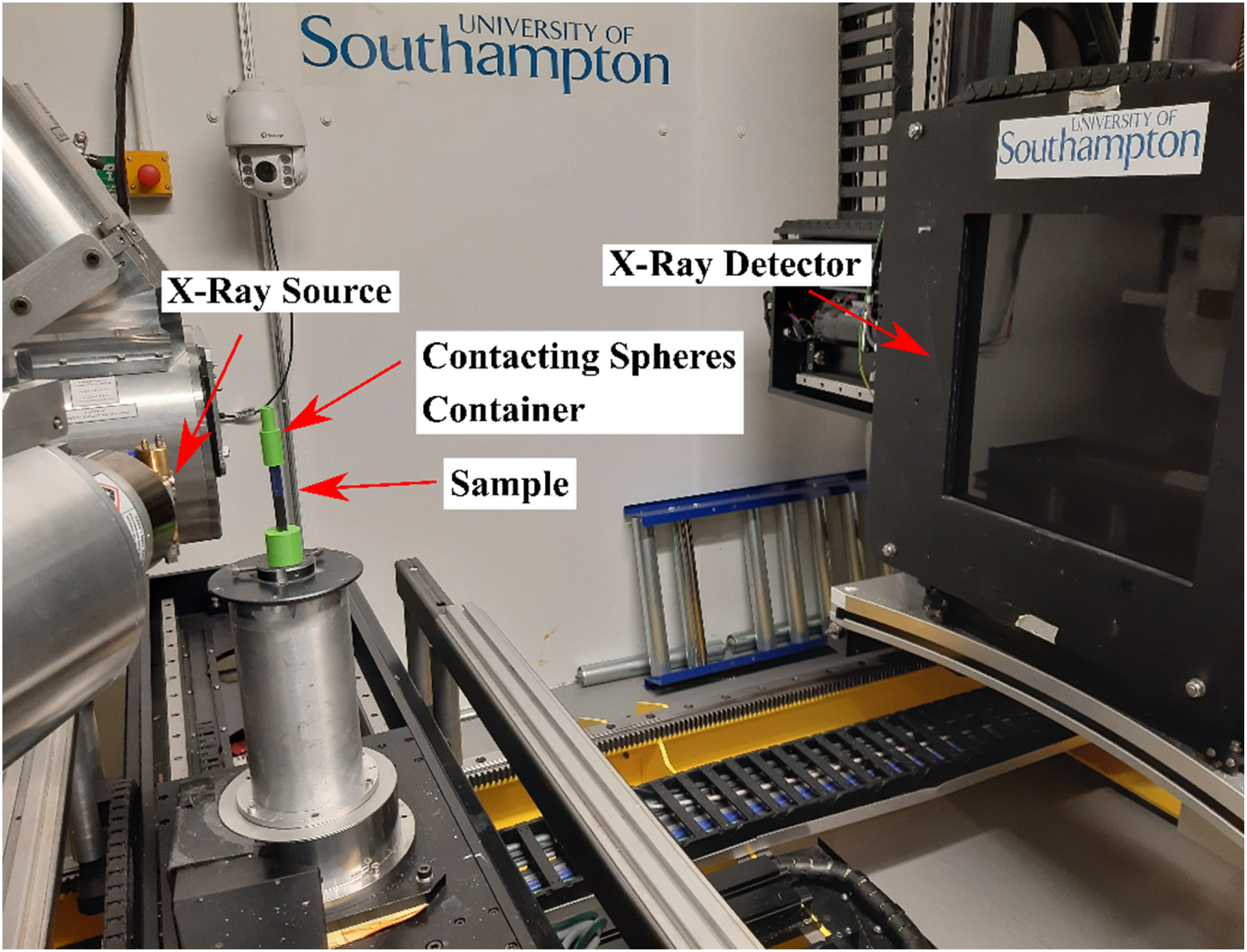

All measurement systems require some sort of assessment of their resolution and noise. Prior to starting the set of scans for each resolution, the XCT machine geometry was verified by scanning contacting ruby spheres (6 mm diameter) placed in a custom holder that was mounted on top of the sample. Voxel size verification was also performed. Details of the system verification results are provided in Appendix A of the supplementary information.

The proposed selection of the XCT parameters includes scanning of the sample at four voxel resolutions (6, 15, 25 and 50 µm) and at six scan times (0.5, 1, 2, 4, 8 and 60 min) for each resolution. Additional scans were performed at 6 µm for 120 min and 420 min to assess the system baseline signal-to-noise ratio. In total, 26 scans were performed and the full text matrix is shown in Table 1.

Table 1.

CT Parameters selection.

Resolution (µm)	Scan time (min)	Exposure (ms)	Projections	Frames per projection	Power (W)	Voltage (kV)
6	420 (baseline)	500	3143	16	10	160
	0.5	354	85	1	6	160
	1		170	1
	2		340	1
	4		680	1
	8		1360	1
	60		5000	2
	120		5000	4
15	0.5	177	170	1	14	160
	1		340	1
	2		680	1
	4		1360	1
	8		2720	1
	60		5000	4
25	0.5	177	170	1	26	160
	1		340	1
	2		680	1
	4		1360	1
	8		2720	1
	60		5000	4
50	0.5	177	170	1	50	160
	1		340	1
	2		680	1
	4		1360	1
	8		2720	1
	60		5000	4

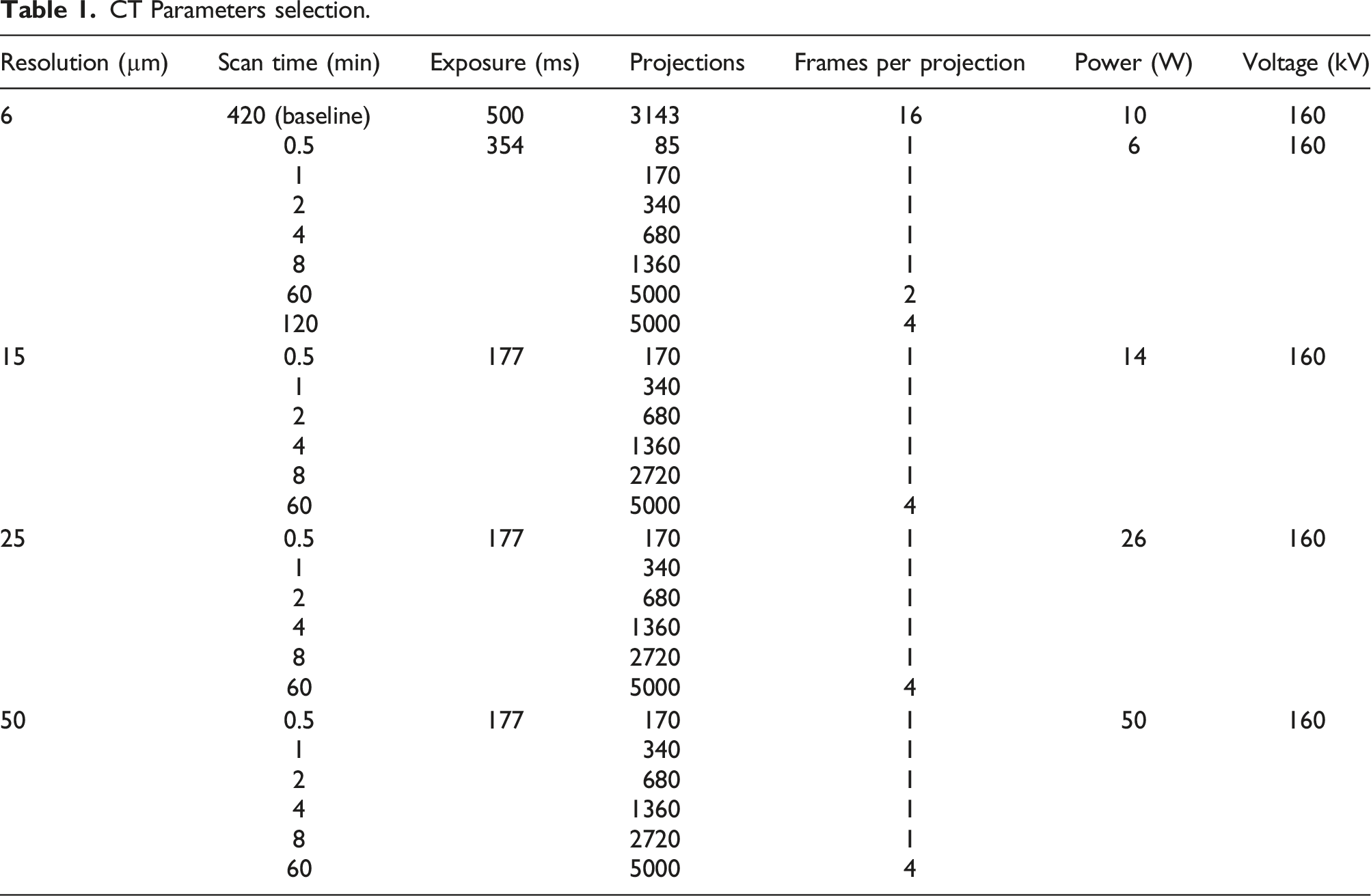
The choice of resolution and scan time was based on the physical limitations of the XCT hardware, which can reach a minimum scan time of 30 s and a maximum resolution of 6 µm for the chosen sample dimensions. With regards to resolution, 15 µm was selected as it is comparable to the voxel size previously used in the literature,^6,8 50 µm was set to match the size of the smallest feature of interest, and 25 µm was chosen as a midpoint with a bias towards the resolutions used in literature. Regarding the scan times, 1, 2, 4 and 8 min were chosen as realistic scan times used to capture time-resolved processes, and 60 min is the approximate duration of a scan aiming to characterise porosity in composite samples.^5,19

In keeping with XCT manufacturer supplied data, X-ray power settings were linearly-scaled such that source spot size and voxel size are approximately equal. In addition, for each resolution the power was set so that the spot size matches the voxel size, and the scan time was adjusted via the variation of the frames per projection while the exposure and the gain remained constant. At low power settings, using slightly higher power than the pixel resolution is often done to get an increased signal to noise ratio, which gives more benefit to the end reconstruction. Trials with a Siemens star linear target were done to confirm that 6 µm resolution was achieved at 10 W with an increased signal to noise ratio. Radiographs of the linear target scanned at 6 and 10 W are available in Appendix A of the supplementary information.

Image processing

Each scan was reconstructed by FBP using Nikon CT Pro, generating a 3D image of 2000 × 2000 × 2000 greyscale voxels and then followed the image processing workflow shown in Figure 2. A central sub-volume of 6 mm × 6 mm × 6 mm was extracted from all the scans after rotating and cropping the initial volume. The resulting sub-volumes were converted to 8-bit to reduce computational costs. Special attention was taken to always select the same sub-volume in all the scans. It is worth noting that the number of voxels contained in each of the scans differ due to the difference in resolution. Therefore, the resulting volume of 6 mm × 6 mm × 6 mm is equivalent to a volume of 1000 × 1000 × 1000, 400 × 400 × 400, 240 × 240 × 240 and 120 × 120 × 120 voxels for the 6, 15, 25 and 50 µm scans, respectively.

Figure 2.

Image segmentation workflow, comprising the data acquisition (blue), image pre-processing (red), segmentation (green) and porosity evaluation (grey).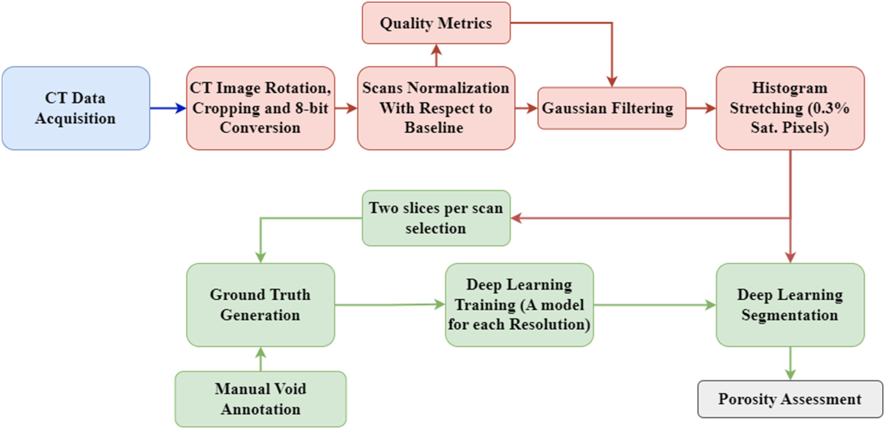

Scan assessment

Since the raw scans were performed under different hardware settings, a difference in their overall quality was observed upon initial inspection. The effect of image processing the raw scans is shown in Figure 3. A three-step image processing routine was implemented in Python 3.6 and Fiji (ImageJ) to facilitate the subsequent feature segmentation and analysis.

Figure 3.

Image pre-processing and segmentation steps for the scans at the different voxel sizes and a constant scan time of 2 min.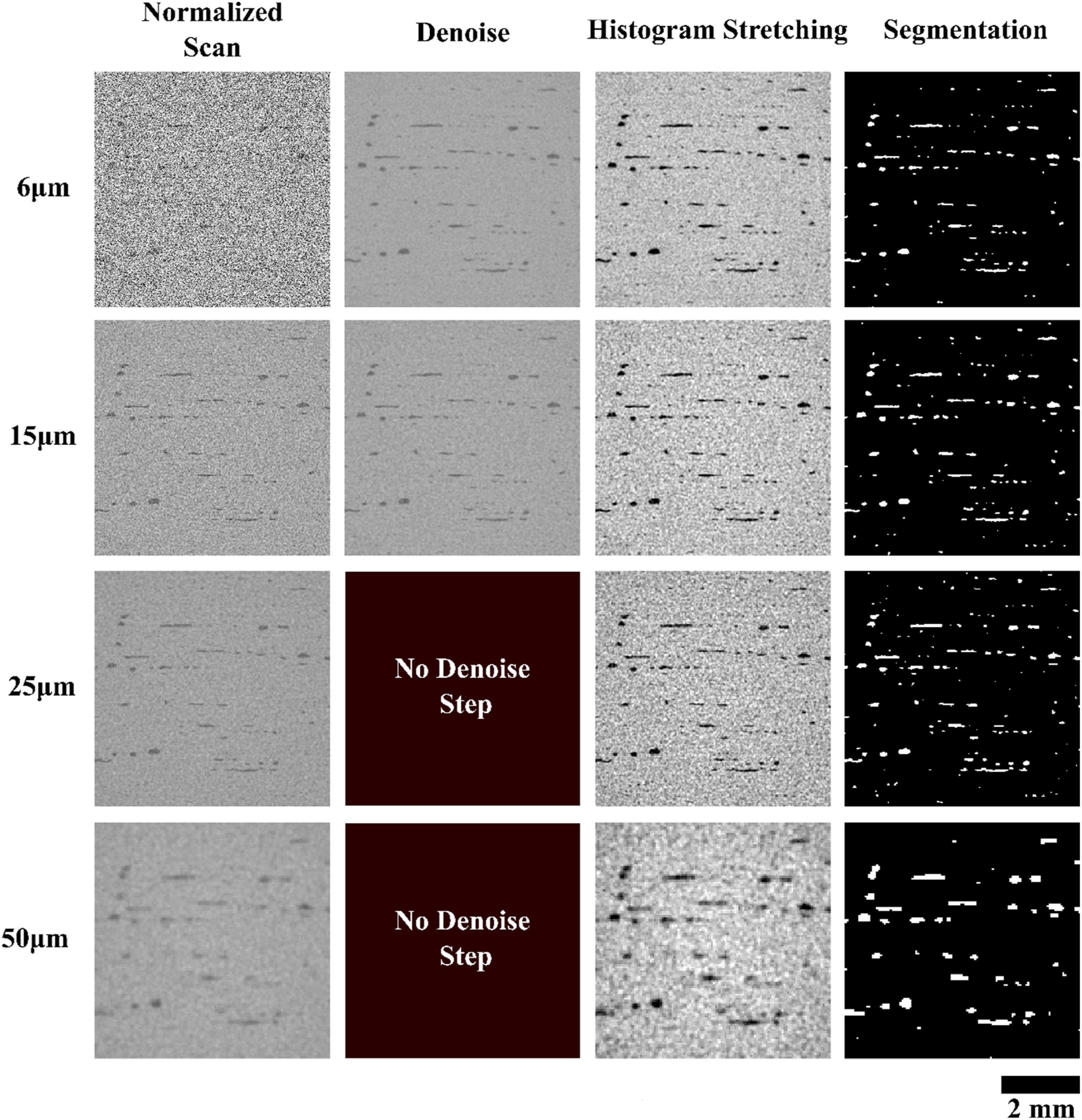

The first step was to normalise the CT data so that the intensities representing both the composite and voids (air) phases are similar across all the scans.²⁰ The grey values corresponding to both phases in the baseline scan were taken as a reference, by extracting the mean grey value in two regions containing exclusively voids or composite. The grey values for both phases were then extracted from the other the scans in the same regions as in the reference scan. The greyscale intensities were normalised with respect to the reference grey values for each scan.

The second step was to denoise the scan.²¹ Denoising was done using a Gaussian denoise filter of variable size, depending on the quality of the input scan. This special case of mean filter²² was successfully used for the denoising of CT data of composite materials in previous studies^6,23,24 and was applied in this study throughout the plugin “3D Gaussian Blur 3D” available in Fiji. However, the application of a denoise filter generates a smoothing of the image, which limits the detection of the smallest features. For this reason, a visual verification was needed to complement the selection of the filter for each scan. Details of the scan denoise and the filter selection is described in Appendix B of the Supplementary Information.

The third and final step was stretching the histogram from the lowest and highest greyscale values to 0 and 255. In this study, 0.3% of voxels were assigned as saturated values. The aim of this step was to facilitate the visual identification of the features of interest (voids) in the subsequent stages of the image processing methodology.

Porosity segmentation

Deep Learning (DL) semantic segmentation, where each pixel in the image is associated to a pre-defined class label, was applied to segment the porosity in each scan. In this study, the DL models are implemented using Convolutional Neural Networks (CNN).²⁵ A typical CNN contains millions of trainable parameters (or weights) and learns to identify the features of interest in a set of raw images throughout an iterative process as it is exposed to the associated reference images. The weights are automatically adjusted to reduce the error between the model predictions and the reference data values during training.²⁶ Once the DL model is trained it can segment the same features in new, previously unseen data.

U-Net²⁷ was the chosen CNN architecture and was implemented in Python 3.6 and Tensorflow 2.5.²⁸ The U-Net architecture has been shown to outperform standard thresholding approaches (e.g., ISO-50%,²⁹ local minima threshold,³⁰ or manual threshold¹⁰) to segment porosity in X-ray CT images¹⁹ and optical micrographs.³¹ To confirm that DL was suitable to segment the XCT data collected here, segmentation by thresholding was also considered, and the results presented and discussed in Appendix C of the Supplementary Information. From the analysis, the DL segmentation approach was found to recognise noise better, in line with the observations made in.³² Since DL provides more consistent and cleaner segmented data than thresholding, DL was chosen to assess porosity in this study.

A DL model was trained for each resolution by using two 2D slices from each of the scans performed at the given resolution. In total, four DL models were trained and applied to the semantic segmentation of voids in their respective set of scans. Training DL models with 2D images despite being applied to the segmentation of 3D data is a standard approach in image analysis of CT data of composite material^33,34 and allows a substantial reduction of the computational effort while having a negligeable effect on the segmentation performance.^35,36 Further details of the DL training procedure is described in Appendix D of the Supplementary Information.

Porosity assessment

Following the segmentation of the voids in the set of scans, the porosity was initially characterised in the entire segmented volume (6 mm × 6 mm × 6 mm) using the Fiji plugin BoneJ, which implements an optimised “3D Connected Components Labelling” algorithm.³⁷ To reduce the impact of noise in the segmentation results, only objects containing three or more voxels are considered. Additionally, two 2D Regions of Interest (ROI) with dimensions 3 mm × 0.67 mm were selected in the central slice of the entire volume in the baseline scan, as shown in Figure 4. The two ROIs contain different levels of voids that are representative of high porosity (ROI 1) and low porosity (ROI 2) that need to be detected in high-performance composite laminates, such as those used in aerospace applications. Additionally, ROI 1 is characterised by visually larger and irregular meso-pores, while small and needle-shape interlaminar voids are predominant in ROI 2. The ROI dimensions were chosen so that each ROI contains enough void instances of objects within a representative size range to enable general observations. Furthermore, the same dimensions were selected for both ROIs so that consistent comparisons can be made. All values of porosity were calculated in volume percentage (vol.-%).

Figure 4.

Baseline scan and ROI location in the greyscale (a) and segmented mask using DL (b). ROI 1 and ROI 2 are displayed in red and yellow, respectively.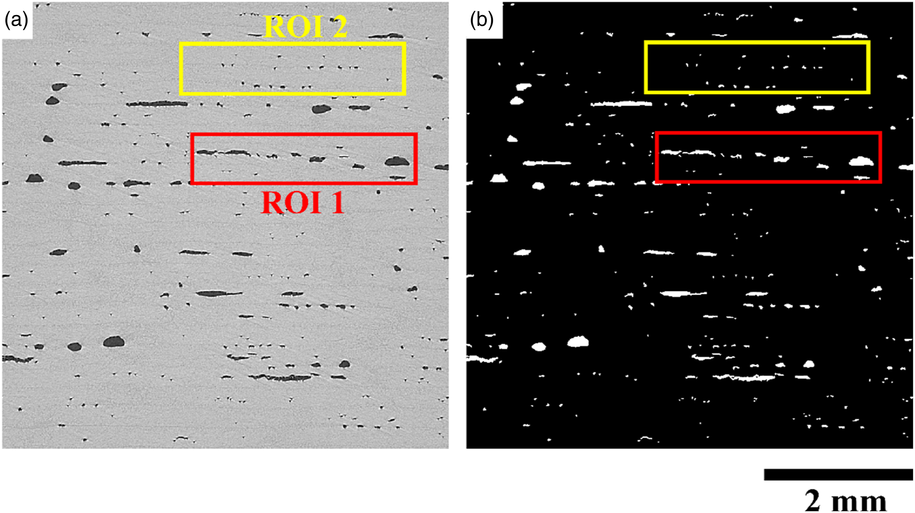

Results

Entire scan porosity assessment

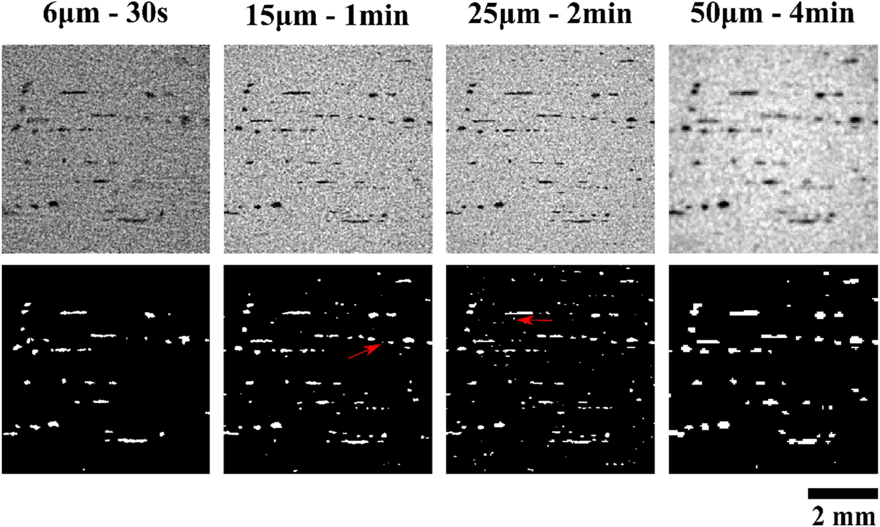
The quantitative characterisation by DL of the porosity in the scans is summarised in Figure 5 and selected segmentations are presented in Figure 6.

Figure 5.

Porosity characterisation for each scan after DL segmentation. The horizontal black line marks the porosity characterisation for the baseline scan after DL segmentation.

Figure 6.

Greyscale scans (top) and segmentation (bottom) of scans at different resolutions and scan times. Red arrows point to examples of objects identified as noise.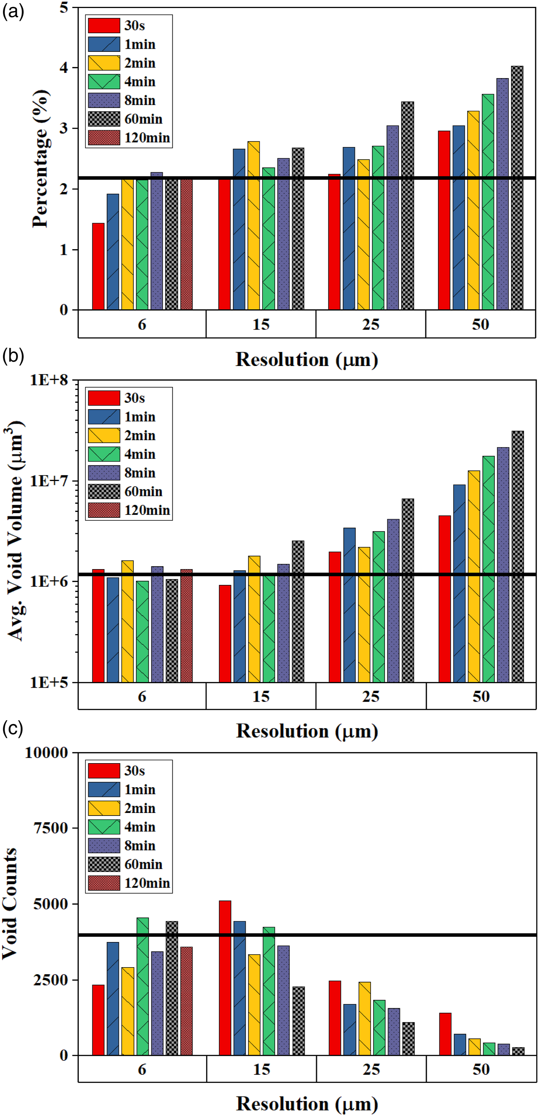

Of the scans performed at a resolution of 6 µm, the porosity, void volume and void count seem to converge towards a relatively constant value for scans lasting 8 min or longer. The signal-to-noise of this XCT system cannot get any better. Therefore, the scan at a resolution of 6 µm lasting 420 min is defined as the baseline for this study.

The baseline scan showed a porosity of 2.18%, with an average void volume of 1.19 × 10⁶ µm³ and a void count of 3976. As resolution decreased from 6 µm to 50 µm, a larger total void content is generally returned, although the number of voids counted is dramatically reduced with smaller voids no longer being detected as fewer voxels cover the scan volume. The fastest scans performed at 6 µm were seen to underestimate the porosity, specifically the 30 s (1.44%) and 1 min (1.92%) scan times. These short scans only capture a few of the large voids and miss most of the medium and small-sized voids, as can be seen in Figure 6.

The scans carried out at 15 µm report a similar porosity level, with an average value of 2.53 ± 0.23%. Increasing the scan time increases the average void volume, from 9.23 × 10⁵ µm³ (30 s scan) to 2.54 × 10⁶ µm³ (60 min scan), together with a decrease of the void counts, from 5124 to 2286. This result implies that as scan time increases, the void segmentation also improves, and therefore a lower amount of noise is captured. Noise can be observed through inspection of the segmented scans shown in Figure 6, where small objects have been segmented but do not match to any of the actual voids existing in the XCT images.

As the voxel size continues to increase, fewer voxels are included in the scan volume. At 25 µm, the equivalent voxel volume is 240 × 240 × 240, which represents a decrease of 72 times compared to the number of voxels in the volume at 6 µm. As noted above, scans at this lower spatial resolution yield a higher apparent porosity content on average than at 15 µm. As the scan time increases, the porosity overestimation also increases, with the lower value provided by the scans done at 30 s (2.25%) and the highest porosity (3.44%) reported at a scan time of 60 min. This increase in the porosity values is accompanied by an increase in the average void volume and a decrease of the void count, due to the reduction of noise because of longer exposure times (i.e., fewer noise-related features being identified as voids).

A substantial overestimation of the porosity is observed in the scans performed at 50 µm, regardless of the scan time. Furthermore, at a resolution of 50 µm, small voids, otherwise captured at other voxel sizes, are completely missed. This effect can be observed in the segmentation of the 4-min scan shown in Figure 6. At 50 µm resolution, a volume of 120 × 120 × 120 voxels is used to represent the scan volume, therefore a single voxel at 50 µm captures a volume approximately six hundred times larger than a voxel at 6 µm. The void count again decreases with the scan time, whereas the average void volume steadily increases and reaches a value of 3.13 × 10⁷ µm³ for the 60 min scan.

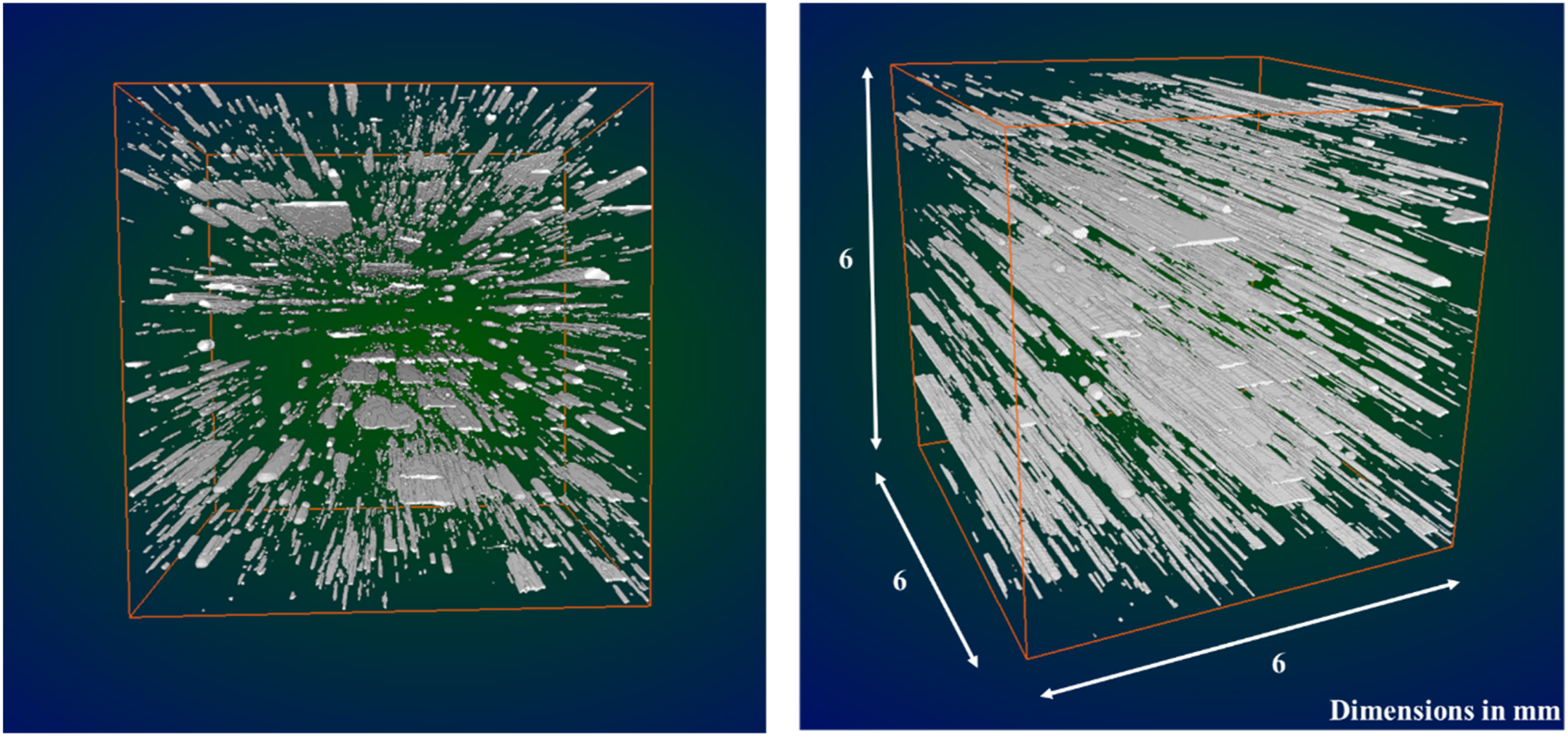
Finally, the 3D rendering of the baseline scan is presented in Figure 7. Flat and elongated voids, as well as needle-shaped voids, are predominant in the volume. It is worth noting that although void segmentation was performed in each of the 2D slices of the 3D volume, continuity in the segmentation of voids spanning several slices is observed and confirms the suitability of the strategy used for the training of the DL model and subsequent scan segmentation.

Figure 7.

3D void distribution in the baseline scan. Front view (a) and perspective view (b). 3D renderings were generated with Dragonfly® 2021.3.1.³⁸

Regions of interest

The effect of XCT scan resolution and scan time on void detection are analysed in the two ROIs, which contain different void distributions.

ROI 1

ROI 1 returns a baseline porosity of 4.95%, containing 16 small and medium-sized segmented voids, with an average void surface of 6178.5 µm². The porosity characterisation provided by the set of scans is displayed in Figure 8.

Figure 8.

Porosity characterization in ROI 1. The horizontal black line marks the baseline scan.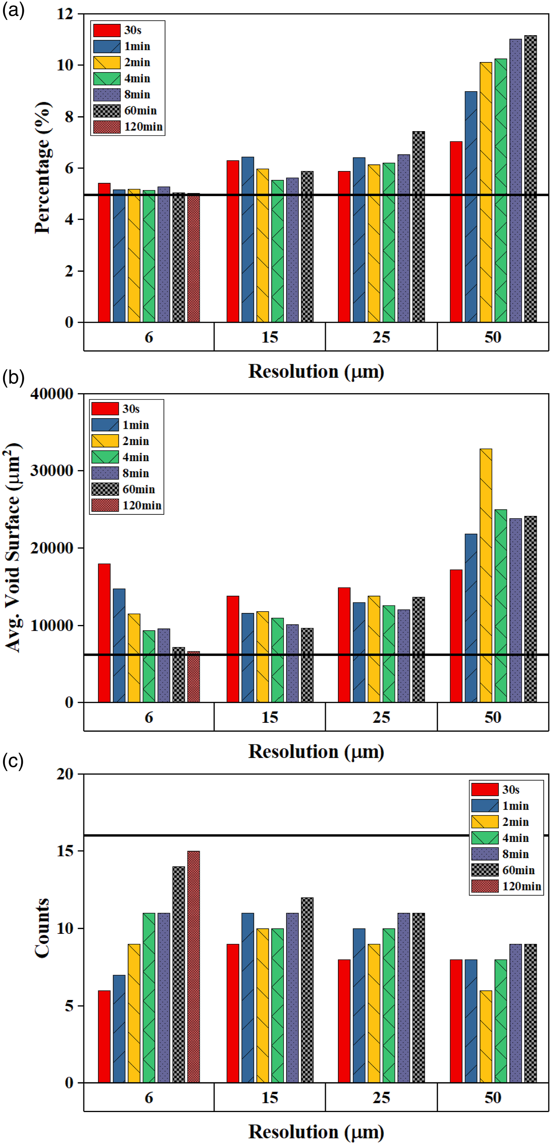

All scans were able to capture the larger voids located at the mid-plane of the ROI, as shown in Figure 9. However, the accuracy of the void segmentation, with respect to the baseline scan, is highly influenced by the CT parameters selection. Two trends can be recognised from a visual and quantitative analysis standpoint: as the scan time increases for a given resolution the number of voids as well as the segmentation precision increases. For instance, the 30 s scan at 6 µm resolution provides an estimated porosity of 5.41%, just 9% higher than the baseline value. However, only six voids are captured, as the smallest voids are missed whilst the average void surface was reported to be 191% higher (18,030 µm² vs 6178.5 µm²). At 120 min, the porosity (5.02%) and the average surface (6688.8 µm²) become closer to the baseline value and a higher number of voids are captured (15 counts), resulting in a more accurate segmentation. This trend was also observed for the 15 µm, 25 µm and 50 µm resolutions.

Figure 9.

Segmentation of the voids in the ROI 1. The red contour marks the segmented voids overlapped to the greyscale image.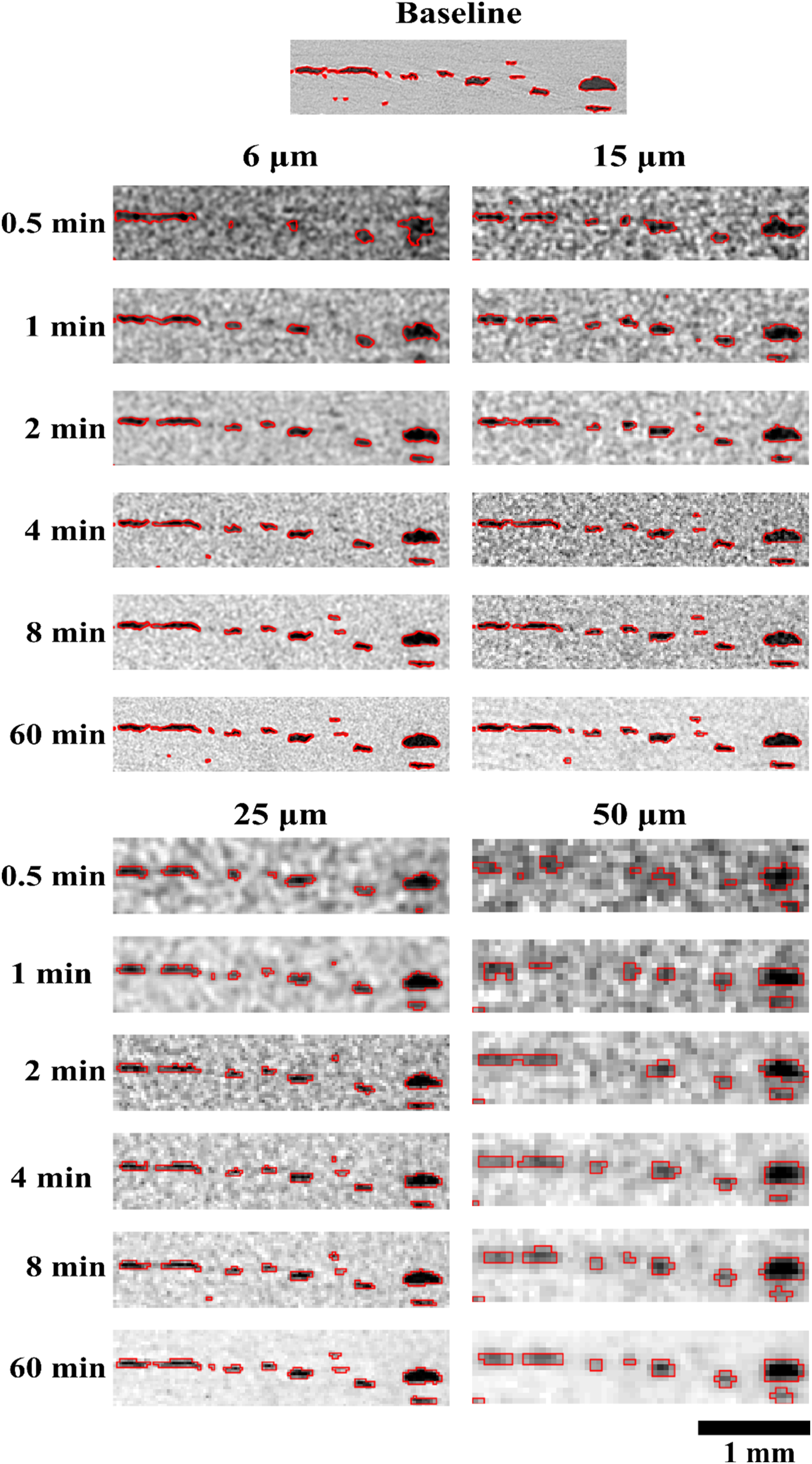

The images in Figure 9 highlight the effect of increased the voxel size. Lower voxel sizes, such as 6 µm or 15 µm provides a finer segmentation of the voids compared to 25 µm and 50 µm. This effect is underscored by the red contour showing the overlap between the segmented mask and the surrounding material in Figure 9. At high resolutions, or lower voxel sizes, the contour appears to closely follow the void edges, providing a high level of detail. However, as the voxel size increases, the level of detail decreases, the red contour becomes coarser and the segmentation accuracy decreases. Additionally, owing to the loss of segmentation accuracy related to a resolution and/or scan time reduction, two neighbouring and elongated voids located at the left-hand side of the baseline ROI are segmented as a single large void in certain scans. This effect correlates to the quantitative overestimation of the maximum void width observed in Figure 8.

ROI 2

This ROI contains a baseline porosity of 0.96% and includes 19 small-sized voids. The average void surface was 1011.8 µm². The quantitative analysis of the porosity characterisation estimated for each scan is presented in Figure 10.

Figure 10.

Porosity characterization in ROI 2. The horizontal black line marks the baseline scan.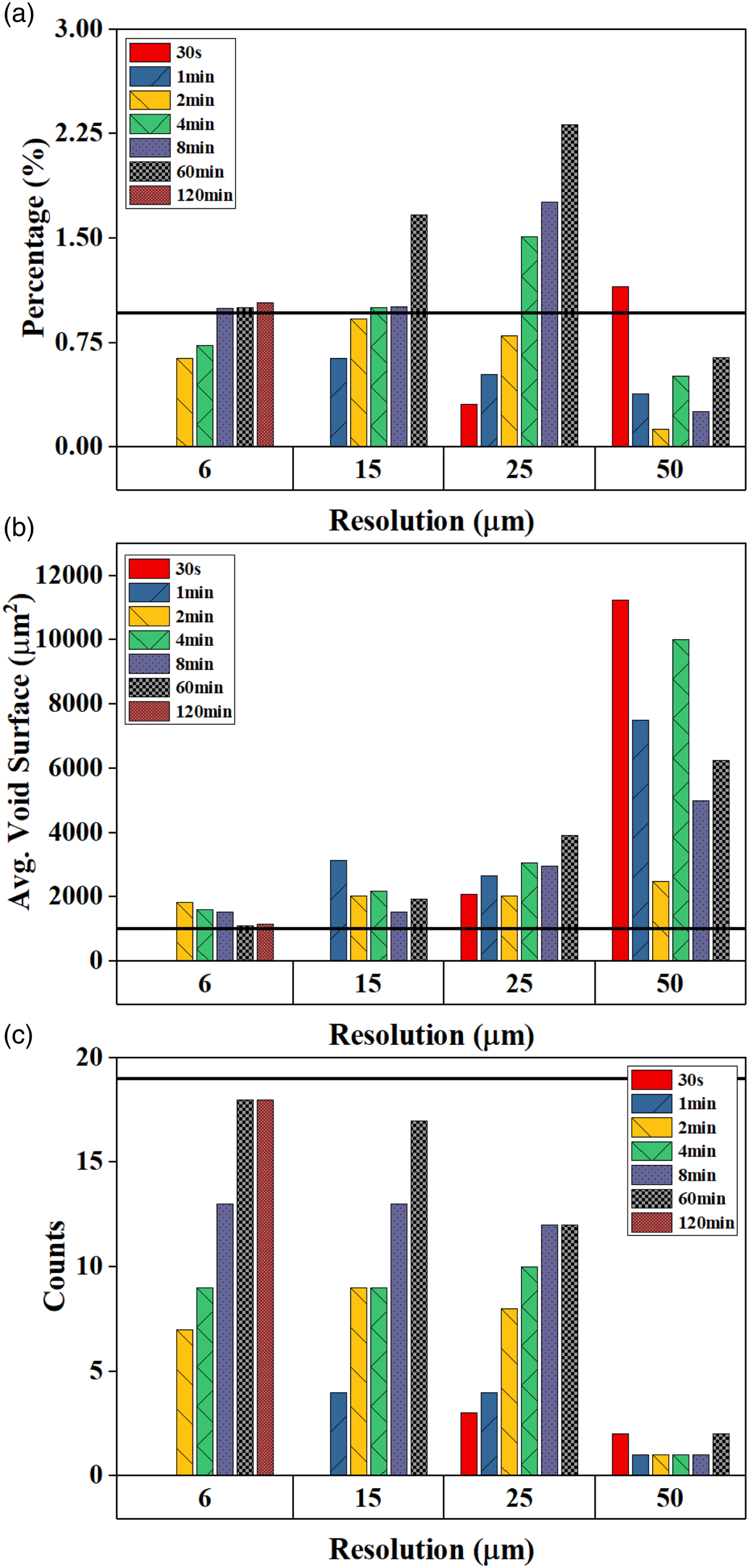

The effect of reducing the scan time on the segmentation of such small voids is that the shortest scan times of 30 s completely miss the voids for resolutions of 6 µm and 15 µm microns. Void segmentation in the 25 µm and 50 µm resolution scans is inadequate for high-performance composites. Most of the scan times shorter than 2 min display a high level of noise represented by a strong fluctuation of the grey level intensity in the entire ROI. The presence of noise and the subsequent use of denoise filters to smooth the image affect the identification and segmentation of small voids in these scans.

As the scan time increases, a higher portion of voids is captured for each resolution. The closest value to the baseline porosity is provided by the 8 min scan at 6 µm (1%), driven by an overestimation of the voids surface since only 13 voids are captured. The 60 and 120 min scans at 6 µm achieve a relative porosity error of only 4.46% and 7.7%, while providing the closest number of void counts and a void segmentation closer to the baseline.

The porosity estimation sharply decreases at 6 µm (30 s and 1 min) and 15 µm (30 s), when compared to the baseline results, as these scan setting are unable to capture any porosity. At these short scan times, either the smaller voids were not captured due to the quality of the 3D image, or their presence has been partially removed by the filtering effect. As the scan time increases, the use of a denoise filter was not deemed necessary due to the improvement of the quality of the raw scans and therefore, the information regarding small voids was preserved.

The largest overestimation of porosity was seen in the 60 min scan at 25 µm, as the estimated voidage level is 140% higher than the reference value. However, from visual assessment of the qualitative results (Figure 11), a relative high number of voids, with a reasonably high segmentation accuracy, are captured. The reason between the mismatch between the quantitative and qualitative results resides in the overestimation of the void volume for each of the voids caused by a coarser segmentation compared to a finer segmentation provided by lower voxel sizes. As a result, since a single voxel at 25 µm occupies a surface of 625 µm², any additional voxel segmented as a void has an impact which is 17 times larger than it has at 6 µm for a ROI surface of 2 mm².

Figure 11.

Segmentation of the voids in the ROI 2. The red contour marks the segmented voids overlapped to the greyscale image.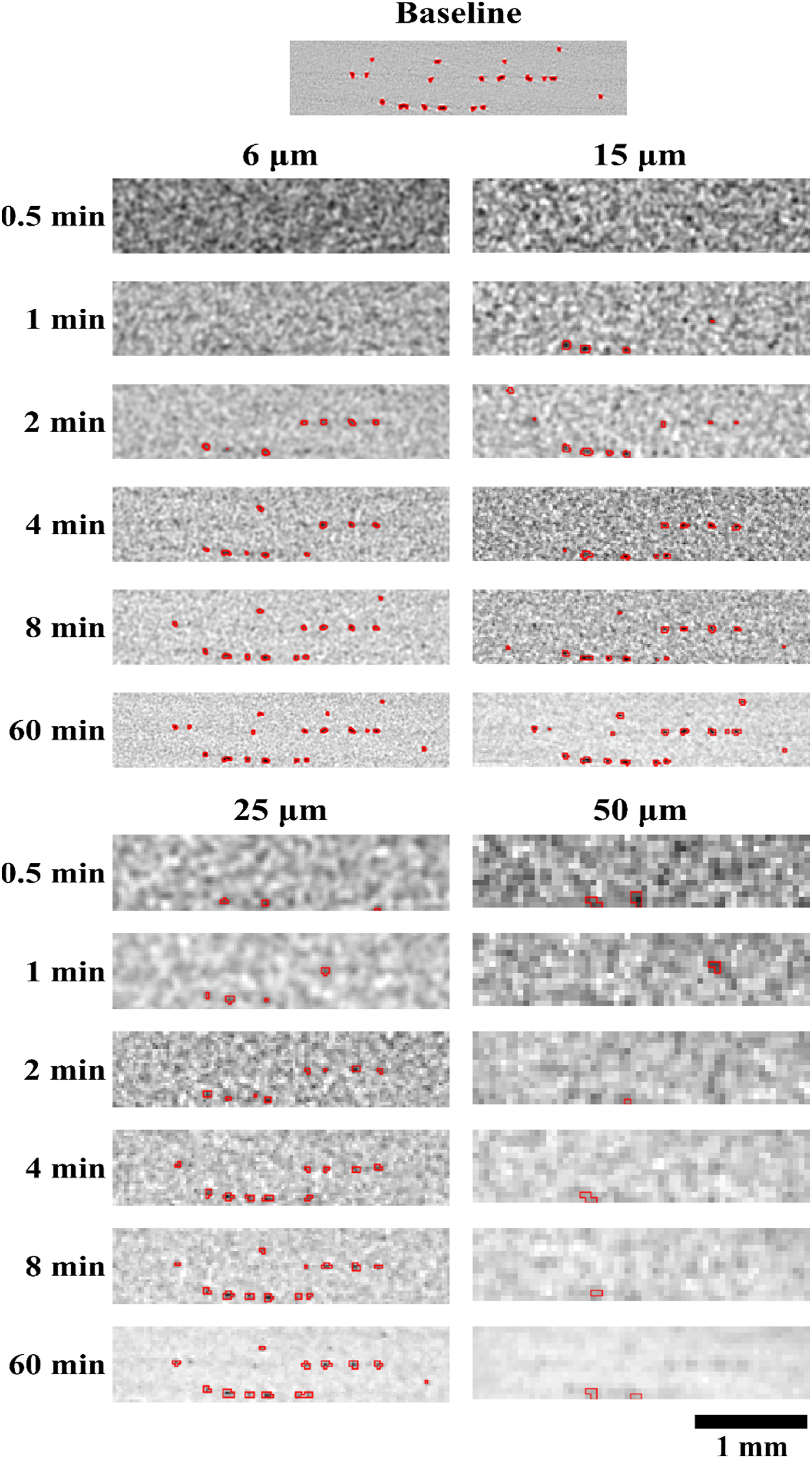

At 50 µm the surface covered by a single voxel is 2.5 times larger than the average void surface (2500 µm² vs 1011.8 µm²) and therefore a large inaccuracy in the detection of voids was observed, resulting in an underestimation of the number of voids for all scans as well as a loss in the precision of the segmentation. This effect is illustrated by the average surface obtained by the scans performed at 1, 2, 4 and 8 min, where a single void was segmented and with a surface of 7500 µm², 2500 µm², 10,000 µm² and 5000 µm², respectively.

Discussion

The results confirm literature reports that the selection of XCT scan conditions have a strong effect on the porosity estimation relevant to composite laminates. The biggest discrepancies in terms of porosity values were found in the scans at 50 µm (Figure 5), where an overestimation of the porosity by more than 80% was observed at the longest scan time, in line with the results generated in previous studies.¹⁵ The scans carried out at 6 µm showed a degree of consistency and convergence with increasing scan time, with the shortest scan showing the biggest deviation with respect to the baseline values. At 15 µm, most of the scans show a constant overestimation of the porosity, whereas increasing the scan time above the 4 min threshold at 25 µm, increases the porosity as bigger voids are overestimated.

A closer inspection of the Regions of Interest containing high (ROI 1), and low (ROI 2) porosity allows a detailed analysis of the effect of the CT parameters in such areas and the impact of the void morphology and size in the segmentation performance.¹⁷ Short scan times (equal or less than 2 min) were found to detect relatively large voids (>300 µm width), whereas it hampered the segmentation of the voids with a width smaller than 100 µm. The presence of noise in shorter scan times made segmentation of smaller voids difficult.

Larger voids (>300 µm width) are captured by all scan times at any resolution. However, the segmented void volume has shown a substantial sensitivity to the choice of resolution. It was noted that at high voxel sizes, particularly at 50 µm, the overestimation of porosity is mainly driven by the partial volume effect,^39,40 occurring when two or more phases, with different densities, are captured by a single voxel. Therefore, the resulting voxel intensity is related to the weight average of the attenuations of each of the constituent materials. The effect of this feature in the porosity assessment is exaggerated by the coarse segmentation of the voids at low resolutions, compared to the results produced at smaller voxel sizes. A similar effect was reported in.⁴¹

The presence of partial volume effects dominated the segmentation of voids at the 50 µm scan resolution, as observed in Figure 9. The comparison of a single raw and segmented void in the baseline and in the 60-min scan at 50 µm is illustrated in Figure 12. This void occupies a surface of 2.96 × 10⁴ µm² (824 voxels) and displays a finer segmentation in the baseline scan, whereas a highly pixelated void, covering a surface of 6.5 × 10⁴ µm² with only 26 voxels is obtained at 50 µm. The decrease in the resolution and the partial volume effects entails a coarser segmentation and the void volume overestimation.

Figure 12.

Effect of scan resolution on the void volume greyscale image and segmentation of the same void in the baseline scan at 6 µm (a) and in the 60-min scan at a voxel size of 50 µm (b). Both segmentation masks are overlapped to the void in the baseline scan (c).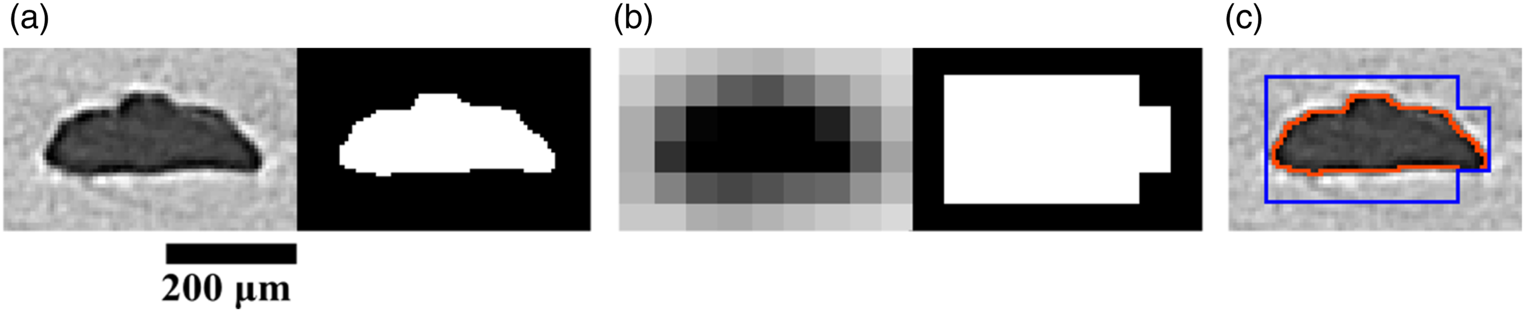

Conclusion

The influence of XCT scan parameters on the porosity evaluation in composite laminates was analysed by scanning a cured composite sample in 26 different combinations of resolution and scan time. The data was collected using a conventional laboratory-based XCT measurement system that was suitably cross-checked, as described in the supplementary information Appendix A.

Higher resolution and longer scan times were observed to provide better quality images for porosity segmentation due to a reduction in noise. Shorter scan times at high resolution require relatively aggressive filters to reduce the effects of noise, and as a consequence, distort the image and remove information associated with small-sized voids. The resolution decrease involves a reduction in the severity of the noise as more X-ray counts are captured in the same volume of material, but the use of filters was still deemed necessary for certain scans. It has been observed that an increase of the voxel size entails a porosity overestimation mainly driven by the presence of partial volume effects, which reduces the segmentation accuracy because of the loss of detail.

Deep Learning and thresholding segmentation were used to analyse the porosity level within reconstructed XCT data. Both Deep Learning and thresholding work well for datasets having a high signal to noise ratio. Deep Learning was found to increase the probability of detecting true porosity data in lower quality (i.e. noisier) scans (e.g. those performed in 1 to 8 min) by capturing a wider range of void sizes and limiting the porosity overestimation induced by the partial volume effects. However, Deep Learning is limited by the quality of the data in the training set, therefore the important influence of scan time on the resulting signal to noise is better quantified in this study. These results can be used to increase the capacity of XCT systems, reduces single scan costs, and open opportunities to observe time-resolved events.

Supplemental Material

Supplemental Material - The effect of X-ray computed tomography scan parameters on porosity assessment of carbon fibre reinfored plastics laminates

Supplemental Material for The effect of X-ray computed tomography scan parameters on porosity assessment of carbon fibre reinfored plastics laminates by Pedro Galvez-Hernandez, Ronan Smith, Karolina Gaska, Mark Mavrogordato, Ian Sinclair and James Kratz in Journal of Composite Materials.

Footnotes

Declaration of conflicting interests

The author(s) declared no potential conflicts of interest with respect to the research, authorship, and/or publication of this article.

Funding

The author(s) disclosed receipt of the following financial support for the research, authorship, and/or publication of this article: The authors would like to acknowledge the Engineering and Physical Sciences Research Council (EPSRC) for their support of this research through Investigation of Fine-Scale Flows in Composites Processing [EP/S016996/1]. XCT imaging was supported by the EPSRC National Research Facility for Lab X-ray CT (NXCT) at the µ-VIS X-ray Imaging Centre, University of Southampton [EP/T02593X/1]. A PhD studentship for P. Galvez-Hernandez was supported through the Rolls-Royce Composites University Technology Centre at the University of Bristol.

ORCID iDs

Pedro Galvez-Hernandez

Ronan Smith

James Kratz

Data availability statement

The raw CT data used in this study is available from the University of Bristol research data repository, data.bris, at .

Supplemental Material

Supplemental material for this article is available online.

References

Naresh

Khan

Umer

, et al. The use of X-ray computed tomography for design and process modeling of aerospace composites: a review. Mater Des 2020; 190: 108553.

Garcea

Wang

Withers

. X-ray computed tomography of polymer composites. Compos Sci Technol 2018; 156: 305–319.

Schofield

King

Tayal

, et al. Image reconstruction: part 1 – understanding filtered back projection, noise and image acquisition. J Cardiovasc Comput Tomogr 2020; 14(3): 219–225.

Hanke

Fuchs

Salamon

, et al. 3 - X-ray microtomography for materials characterization. In: Hübschen

Altpeter

Tschuncky

, et al. (eds) Materials characterization using nondestructive evaluation (NDE) methods. Sawston, UK: Woodhead Publishing, 2016. pp. 45–79.

Mehdikhani

Straumit

Gorbatikh

, et al. Detailed characterization of voids in multidirectional carbon fiber/epoxy composite laminates using X-ray micro-computed tomography. Compos Appl Sci Manuf 2019; 125: 105532.

Dilonardo

Nacucchi

De Pascalis

, et al. High resolution X-ray computed tomography: a versatile non-destructive tool to characterize CFRP-based aircraft composite elements. Compos Sci Technol 2020; 192: 108093.

Little

Yuan

Jones

. Characterisation of voids in fibre reinforced composite materials. NDT E Int 2012; 46: 122–127.

Kratz

Galvez-Hernandez

Pickard

, et al. Lab-based in-situ micro-CT observation of gaps in prepreg laminates during consolidation and cure. Compos Appl Sci Manuf 2021; 140: 106180.

Torres

Simmons

Sket

, et al. An analysis of void formation mechanisms in out-of-autoclave prepregs by means of X-ray computed tomography. Compos Appl Sci Manuf 2019; 117: 230–242.

10.

Centea

Hubert

. Measuring the impregnation of an out-of-autoclave prepreg by micro-CT. Compos Sci Technol 2011; 71(5): 593–599.

11.

Bradley

Soutis

, et al. A comparison of different approaches for imaging cracks in composites by X-ray microtomography. Philos Trans A Math Phys Eng Sci 2016; 374(2071): 20160037.

12.

Lambert

Chambers

Sinclair

, et al. 3D damage characterisation and the role of voids in the fatigue of wind turbine blade materials. Compos Sci Technol 2012; 72(2): 337–343.

13.

Stoessel

Denis Diewel

, et al. µ-computed tomography for 3D porosity evaluation in carbon fibre reinfored plastics (CFRP). International symposium on digital industrial radiologyand computed tomography. Berlin, Germany, 20–22 June 2011.

14.

Plank

Mayr

Reh

, et al. Evaluation and visualisation of shape factors in dependence of the void content within CFRP by means of X-ray computed tomography. European conference on non-destructive testing (ECNDT 2014), Prague, Czech Republic, 6–11 October 2014, 2016.

15.

Kiefel

Stoessel

Plank

, et al. CFRP porosity characterisation using µ-Computed Tomography with optimized test parameters supported by XCT-simulation. Conference on industrial computed tomography (iCT2014), Wels, Austria, 25–28 February 2014.

16.

Kastner

Plank

Salaberger

, et al. Defect and porosity determination of fibre reinforced polymers by X-ray computed tomography. 2nd international symposium on NDT in aerospace, Hamburg, Germany, 22–24 November 2010.

17.

Plank

Sause

MGR

Kastner

. High-resolution X-ray computed tomography simulations of synthetically-generated volume porosity in continuous carbon fibre-reinforced polymer samples. Nondestr Test Eval 2022; 37: 645–665.

18.

Zwanenburg

Williams

Warnett

. Review of high-speed imaging with lab-based x-ray computed tomography. Meas Sci Technol 2021; 33(1): 012003.

19.

Galvez-Hernandez

Gaska

Kratz

. Phase segmentation of uncured prepreg X-ray CT micrographs. Compos Appl Sci Manuf 2021; 149: 106527.

20.

Voigt

Miller

Mainza

, et al. The robustness of the gray level co-occurrence matrices and X-ray computed tomography method for the quantification of 3D mineral texture. Minerals 2020; 10(4): 334.

21.

Hung

Sun

, et al. How far can the radiation dose be lowered in head CT with iterative reconstruction? Analysis of imaging quality and diagnostic accuracy. Eur Radiol 2013; 23(9): 2612–2621.

22.

Gonzalez

Woods

. Digital image processing. 4th ed. New York, NY: Pearson, 2018.

23.

Ferré Sentis

Orgéas

Dumont

PJJ

, et al. 3D in situ observations of the compressibility and pore transport in sheet moulding compounds during the early stages of compression moulding. Compos Appl Sci Manuf 2017; 92: 51–61.

24.

Dilonardo

Nacucchi

De Pascalis

, et al. Inspection of carbon fibre reinforced polymers: 3D identification and quantification of components by X-ray CT. Appl Compos Mater 2022; 29(2): 497–513.

25.

Goodfellow

Bengio

Courville

. Deep learning. Cambridge, MA: MIT Press, 2017.

26.

LeCun

Bengio

Hinton

. Deep learning. Nature 2015; 521(7553): 436–444.

27.

Ronneberger

Fischer

Brox

. U-Net: convolutional networks for biomedical image segmentation. In: Navab

Hornegger

Wells

, et al. (eds) Medical image computing and computer-assisted intervention – MICCAI 2015. Cham, UK: Springer International Publishing, 2015, pp. 234–241.

28.

Abadi

Agarwal

Barham

, et al. TensorFlow: large-scale machine learning on heterogeneous distributed systems. 2016. https://arxiv.org/abs/1603.04467.

29.

Kruth

Bartscher

Carmignato

, et al. Computed tomography for dimensional metrology. CIRP Annals 2011; 60(2): 821–842.

30.

Gélébart

Chateau

Bornert

, et al. X-ray tomographic characterization of the macroscopic porosity of chemical vapor infiltration SIC/SIC composites: effects on the elastic behavior. Int J Appl Ceram Technol 2010; 7(3): 348–360.

31.

Machado

Tavares

JMRS

Camanho

, et al. Automatic void content assessment of composite laminates using a machine-learning approach. Compos Struct 2022; 288: 115383.

32.

Bellens

Probst

Janssens

, et al. Evaluating conventional and deep learning segmentation for fast X-ray CT porosity measurements of polymer laser sintered AM parts. Polym Test 2022; 110: 107540.

33.

Lorenzoni

Curosu

Paciornik

, et al. Semantic segmentation of the micro-structure of strain-hardening cement-based composites (SHCC) by applying deep learning on micro-computed tomography scans. Cement Concr Compos 2020; 108: 103551.

34.

Badran

Marshall

Legault

, et al. Automated segmentation of computed tomography images of fiber-reinforced composites by deep learning. J Mater Sci 2020; 55(34): 16273–16289.

35.

Fioravante de Siqueira

Ushizima

van der Walt

. A reusable neural network pipeline for unidirectional fiber segmentation. Sci Data 2022; 9(1): 32.

36.

Bertoldo

JPC

Decencière

Ryckelynck

, et al. A modular U-net for automated segmentation of X-ray tomography images in composite materials. Front Mater 2021; 8.

37.

Doube

Michael

. Multithreaded two-pass connected components labelling and particle analysis in ImageJ. BioRxiv. 2021; 8(3). doi:10.1098/rsos.201784

38.

Dragonfly 2021.3.1. Montreal, QC: Comet Technologies Canada Inc., 2021.

39.

Souza

Udupa

Saha

. Volume rendering in the presence of partial volume effects. IEEE Trans Med Imag 2005; 24(2): 223–235.

40.

Bull

Sinclair

Spearing

. Partial volume correction for approximating crack opening displacements in CFRP material obtained from micro-focus X-ray CT scans. Compos Sci Technol 2013; 81: 9–16.

41.

Plank

Schwarting

Senk

, et al. Multiscale and multimodal approaches for threedimensional materials characterisation of fibre reinforced polymers by means of X-ray based NDT methods. International symposium on digital industrial radiology and computed tomography, Fuerth, Germany, 2–4 July 2019.

Supplementary Material

Please find the following supplemental material available below.

For Open Access articles published under a Creative Commons License, all supplemental material carries the same license as the article it is associated with.

For non-Open Access articles published, all supplemental material carries a non-exclusive license, and permission requests for re-use of supplemental material or any part of supplemental material shall be sent directly to the copyright owner as specified in the copyright notice associated with the article.

0.00 MB

3.14 MB