Sage Journals: Discover world-class research

Abstract

The electro-hydraulic composite control system is widely used in industrial equipment. It has the advantages of fast response speed and high load level. Sudden faults would lead to shutdown of the production. These would cause production losses, even the safety accidents. Fault diagnosis can obtain the states of equipment faults, promptly alert when faults occur, reduce accidents, and minimize production losses. Due to the large number of components and few sensors in the electro-hydraulic composite system, the faults of many components often exhibit the same characteristics. This increases the difficulty of troubleshooting. To identify faults that require similar features, a digital twin-driven group fault diagnosis method is proposed for faults with similar symptoms. A functional fault grouping strategy was introduced for grouping faults for diagnosis. A fault diagnosis model was established for inferring faulty components during the diagnosis and re diagnosis process. A digital twin model was established to simulate diagnostic results and verify their correctness. The proposed method is evaluated through application to an electro-hydraulic system. The results indicate that the grouping diagnosis strategy improves diagnostic accuracy by approximately 3%–5%.

Keywords

fault diagnosis digital twin electro-hydraulic control system faults with similar symptoms

Introduction

Literature review

In exiting research, fault diagnosis methods for different categories of components vary significantly and real-time analysis of voltage and current signals serves as the primary method for diagnosing faults in electronic power units.³ Electronic power units typically contain three-phase currents, which are modulated in voltage amplitude by transformers.⁴ Usually, a fixed phase difference exists between the three-phase currents. When a fault occurs in one phase, the time-frequency characteristics of the electrical signals change. By monitoring real-time current signals, these faults can be analyzed.⁵ This approach is widely applied in power plants and power transmission stations, with ongoing optimization and refinement of diagnostic techniques. For instance, robust fault diagnosis techniques are developed for three-phase dual active bridges,⁶ and classification methods are proposed for identifying high-resistance connection faults in switched reluctance motors.⁷ These methods are generally characterized by high accuracy and ease of achieving real-time diagnosis. However, real-time current and voltage detection requires high-quality sensors, which are often expensive. Thus, low-frequency voltage or current sensors are commonly used in complex electro-hydraulic control systems, making it difficult to capture high-frequency signals.

For electronic control systems, a key feature is the control of high-voltage actuators using low-voltage electronic signals.⁸ Fault diagnosis in these units often benefits from multiple monitoring points, because the components such as Programmable Logic Controller (PLC) are equipped with built-in data monitoring functions, reducing the complexity of health monitoring.⁹ Fault diagnosis methods based on fault trees¹⁰ and causal reasoning¹⁰ still face technical challenges, particularly in the development of real-time communication interfaces for various configuration software systems.¹¹ In hydraulic systems, fault diagnosis primarily relies on state recognition through low-frequency hydraulic pressure and flow signals.¹² Typically, the addition of sensors alters the structure of the existing system, potentially impacting the performance of the hydraulic system. As a result, the original sensors in many hydraulic systems often serve as the sole source of information for fault diagnosis. Fault diagnosis under sensor constraints has become an important research focus in recent years. Solutions such as virtual sensors are introduced to enhance diagnostic performance,¹² and methods addressing the limitations of low-accuracy sensors are proposed.¹³

The above analysis demonstrates the significant effectiveness of fault diagnosis methods tailored to individual units within large and complex systems. However, electro-hydraulic systems are characterized by a limited number of sensors and a diverse range of fault types.^14,15 Under these conditions, many faults exhibit similar symptoms, complicating diagnosis. For instance, failures within components of the same hydraulic circuit can lead to abnormal values in specific hydraulic sensor readings, making it challenging to accurately identify the faulty component based solely on the observed anomaly. Furthermore, multiple electronic control components may regulate the same valve, and the failure of any individual component can result in valve control malfunction, posing a significant challenge in pinpointing the specific faulty component. Enhancing the accuracy of fault diagnosis for faults with overlapping symptoms remains a critical challenge that warrants further investigation.

The digital twin model is an effective tool for improving fault diagnosis performance. By providing dynamic virtual simulations, the digital twin model can offer more detailed information to the fault diagnosis system, enhancing diagnostic accuracy.¹⁶ In exiting research, digital twins support fault diagnosis through various methods. One common approach is to use digital twin models to generate sufficient data for training fault diagnosis models. For example, fault data from digital twin models are applied to the diagnosis of bearings¹⁷ and gearboxes,¹⁸ while high-quality data can also be generated through these models.¹⁸ These techniques help address the problem of insufficient training samples and lower the barriers for applying data-driven fault diagnosis methods. However, the ratio of real to virtual data needs further study, as an excessive amount of virtual data can distort the training sample library.¹⁹ Other frameworks involve using digital twin models to display fault diagnosis results²⁰ and obtain real-time diagnostic data,²¹ while verifying diagnostic results through digital twin models has proven effective in improving diagnostic accuracy.²² A key factor in the success of these methods is the availability of sufficient sensors, as they ensure the digital twin model accurately reflects the actual system. The performance of fault diagnosis is influenced by the number of sensors present. However, electro-hydraulic control systems often have a limited number of sensors, and the addition of new sensors is difficult due to the complex working environment.²³ As a result, many faults present similar symptoms, increasing the difficulty of diagnosis. Improving the ability to distinguish between faults with similar symptoms is crucial for enhancing diagnostic accuracy.

Content and contribution

To address this issue, a digital twin-driven group fault diagnosis method is proposed for faults with similar symptoms. The fault diagnosis model is divided according to the control process to minimize interference. A digital twin-based framework, which includes diagnosis, verification, and re-diagnosis, is established to enhance diagnostic accuracy. The effectiveness of the method is studied using an electro-hydraulic system. The results demonstrate that the proposed method effectively addresses faults with similar symptoms.

The contributions are as follows.

(1) A group fault diagnosis method is proposed for faults with similar symptoms.

(2) A fault diagnosis framework with diagnosis, verification, and re-diagnosis is proposed.

(3) 4The relationship between degree of information and accuracy is researched.

Organization of paper

The structure of the paper is as follows: Section 2 introduces the digital twin-driven group fault diagnosis method for faults with similar symptoms. In Section 3, the electro-hydraulic system and its corresponding fault diagnosis model are presented, along with an analysis of its performance. Section 4 concludes the research.

The digital twin driven group fault diagnosis method for faults with similar symptoms

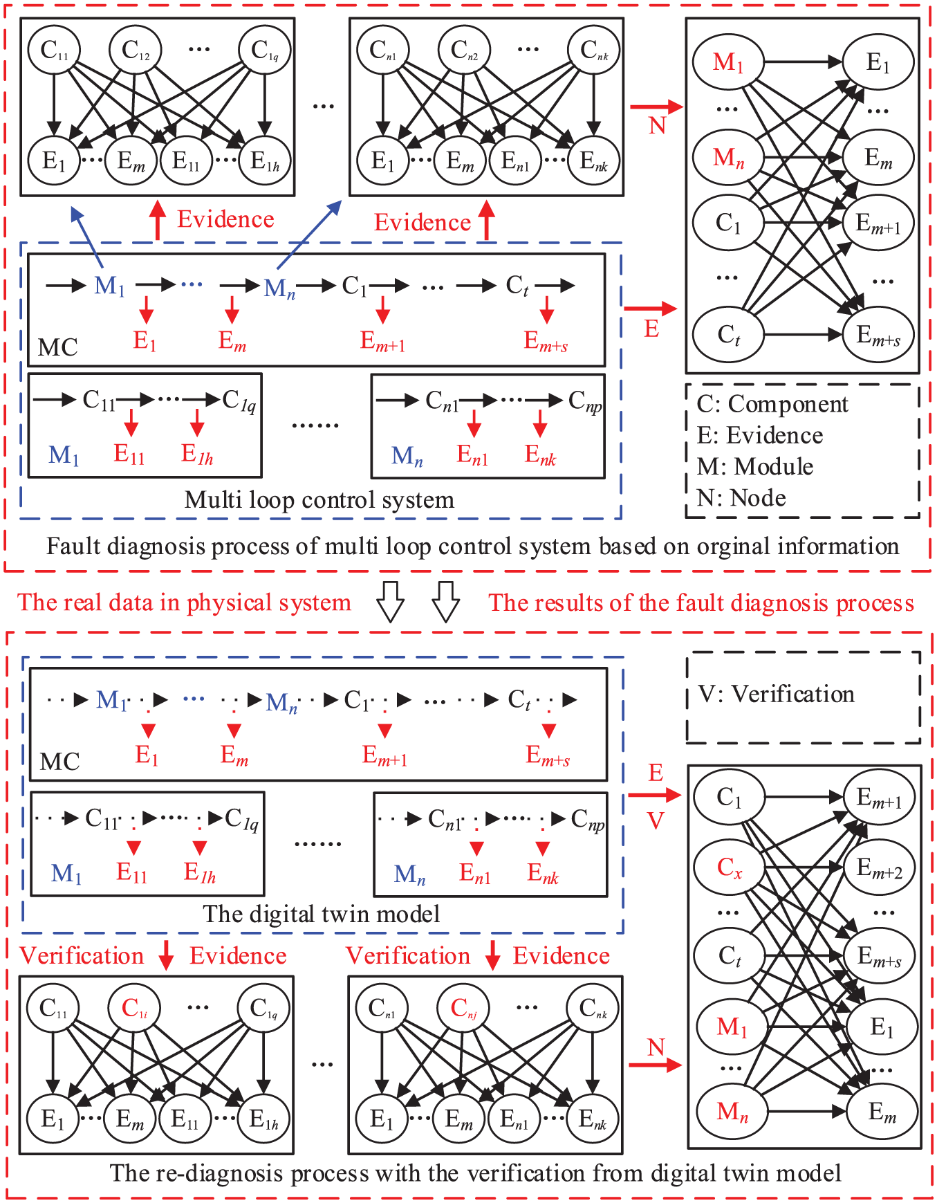
The digital twin driven group fault diagnosis method for faults with similar symptoms is shown in Figure 1. The approach involves two key processes that is, diagnosis and re-diagnosis. During the process of diagnosis, sensor data is collected and fed into the fault diagnosis model. Upon obtaining the diagnostic results, the digital twin model processes this information.

Figure 1.

Digital twin driven group fault diagnosis method for faults with similar symptoms.

If there is a fault, the digital twin model simulates the potential faults and compares the simulated output with the actual system output. The digital twin model aligns with the actual system output, reflecting the result of accurate diagnosis. If discrepancies are detected, the re-diagnosis process is initiated, thereby enhancing diagnostic accuracy. In this fault diagnosis process, the fault diagnosis model is established based on the control flow grouping. When diagnosing faults with similar symptoms, two mechanisms enhance diagnostic accuracy. First, the group modeling approach effectively isolates interference from similar characteristics when diagnosing multiple components, enabling a more targeted analysis of individual components. Second, the diagnosis result verification mechanism, leveraging digital twin technology, significantly reduces the likelihood of incorrect diagnoses.

The fault diagnosis process based on Bayesian Networks

This probability plays a crucial role in updating the fault status of the digital twin model. In a Bayesian Network (BN), the results are got in the form of probability. Usually, the magnitude of probability indicates the possibility of a fault. It is used in fault diagnosis due to good reasoning ability. In the digital twin model, the fault parameter can be updated through these probabilities. Determining the structure of the fault diagnosis model based on BN and providing inference parameters are important steps in establishing a fault diagnosis model.²⁴

In an electro-hydraulic control system, both hydraulic and electronic components are collectively referred to as “components” and their failures can lead to anomalies in measured values. These abnormal data serve as evidence to determine whether a component is malfunctioning. The structure of fault diagnosis models based on Bayesian networks is typically constructed using causal relationships. As illustrated in Figure 1, within each fault diagnosis model, the components act as parent nodes, while the evidence that can be collected from the system forms the child nodes. Evidence generally includes parameters such as voltage in the electronic circuit and oil pressure in the hydraulic circuit. The relationship between parent and child nodes is represented through a conditional probability table, where each probability quantifies the likelihood of the child node’s state under varying conditions of the parent nodes. These probabilities are typically derived through expert decision-making methods.

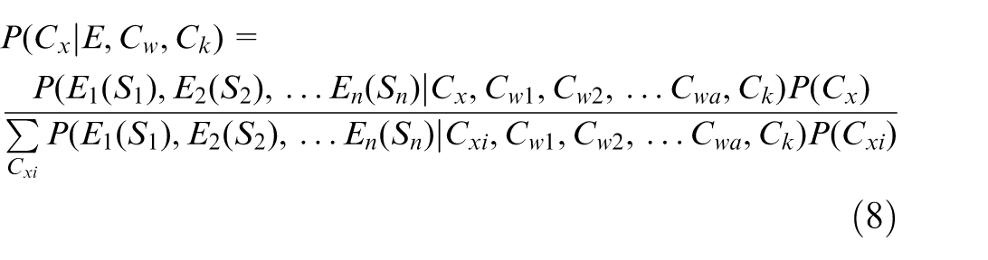
When the evidence (E = E₁(S₁₎, E₂(S₂),…, E_n(S_n)) are got, the probability of a faulty component can be got as follows:

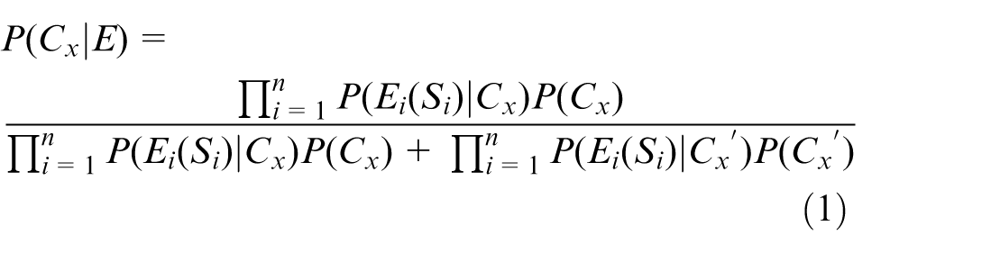
\begin{matrix} P (C_{x} | E) = \\ \frac{Π_{i = 1}^{n} P (E_{i} (S_{i}) | C_{x}) P (C_{x})}{Π_{i = 1}^{n} P (E_{i} (S_{i}) | C_{x}) P (C_{x}) + Π_{i = 1}^{n} P (E_{i} (S_{i}) | {C_{x}}^{'}) P ({C_{x}}^{'})} \end{matrix}

(1)

where, C_x is the x-th component (x = 1, 2,…, m), m is the number of the components. $C_{x}^{'}$ represents that the x-th component is normal. C_x represents that the x-th component is abnormal, n is the number of evidence.

Once the failure probability for each component is determined, a threshold must be established. If the failure probability exceeds this threshold, the component is considered to be abnormal. Typically, this threshold is set at 80%.

The establishment of the digital twin model and verification of the diagnostic results

In an electro-hydraulic control system, the electronic control flow and hydraulic control flow are two critical control paths, each with distinct modeling approaches in the digital twin model. Within the electronic control flow, the voltage (V) signal serves as a key monitoring indicator, and it is typically the output of the digital twin model. An electronic control flow generally comprises components such as switches, PLC, and photoelectric conversion switches. The output of each component is influenced by three main factors that is, the proper input of the control signal, the operational status of the component, and the fulfillment of the working conditions. Consequently, the output of each electronic component can be expressed as follows:²⁶

v_{i} = τ_{i} φ_{i} η_{i} v_{i - 1}

(2)

where, v_i is the output of the i-th component, v_i−1 is the output of i − 1-th component, it is also the input of the i-th component, τ is control parameter, it represents the control signal given to the component at that moment, φ is the fault parameter, it is used to characterize whether this component is faulty, η is the translate parameter, it is used to achieve voltage conversion from the previous component, and it is also used to describe whether the component meets the conditions for normal operation.

Control parameters typically have two possible states, 0 and 1, which are determined by reading control instructions. When the component is an automatic response element, such as a PLC or photoelectric conversion switch, the control parameters are set to 1. This is because these components automatically generate output response values upon receiving input signals.

The calculation method for translate parameter is as follows.

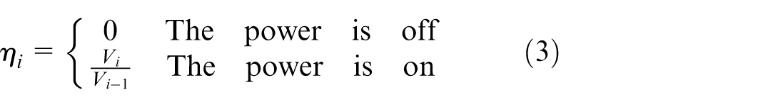
η_{i} = {\begin{matrix} 0 & \begin{matrix} The & power & is & off \end{matrix} \\ \frac{V_{i}}{V_{i - 1}} & \begin{matrix} The & power & is & on \end{matrix} \end{matrix}

(3)

where, the V_i is the output of the i-th component when it is working normally, the V_i−1 is the i − 1-th component when it is working normally.

The calculation method for fault parameter is as follows.

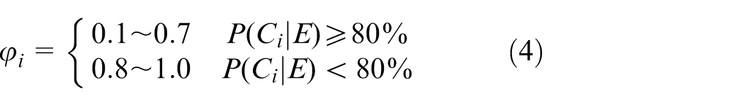
φ_{i} = {\begin{matrix} 0.1 ~ 0.7 & P (C_{i} | E) \geq 80 % \\ 0.8 ~ 1.0 & P (C_{i} | E) < 80 % \end{matrix}

(4)

It can be observed that the fault parameters do not use fixed values; instead, they are typically adjusted based on the specific circumstances to ensure the accuracy of the results. Once selected, the fault parameters under normal conditions remain constant. However, these parameters are modified each time a component is identified as faulty.

For hydraulic control flow, the output is the pressure from the pressure transmitters. Referring to existing research,²⁵ the digital twin model is as follows.

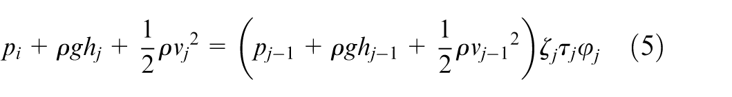
p_{i} + ρ g h_{j} + \frac{1}{2} ρ {v_{j}}^{2} = (p_{j - 1} + ρ g h_{j - 1} + \frac{1}{2} ρ {v_{j - 1}}^{2}) ζ_{j} τ_{j} φ_{j}

(5)

where, p_j is the pressure at the output of the component, p_j−1 is the pressure at the output of the previous component, h is the height of the component, v is the speed of the oil. From the equation, it can be seen that the control parameter and fault parameter are still included, and their calculation methods are consistent with the above method. loss parameter (ζ) is added and it expressed the pressure loss of hydraulic oil. It is got by analysis the history data.

In this research, the digital twin model is used to validate the results of fault diagnosis and provide feedback. For electronic control flow, the calculation method is as follows.

e_{i} = \frac{| v_{i} - v r_{i} |}{v r_{i}} \times 100 %

(6)

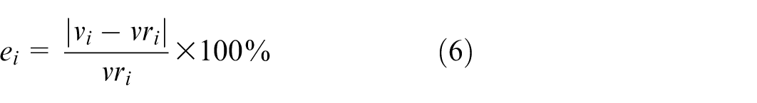
where, e_i is the error between the output of the digital twin model and the output of the electronic control system, vr_i is the actual output voltage of the i-th component.

For hydraulic control flow, the calculation method is as follows.

e_{j} = \frac{| p_{j} - p r_{j} |}{p r_{j}} \times 100 %

(7)

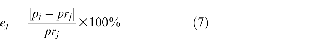
where, pr_j is the actual output pressure of the j-th component.

The re-diagnosis based on the verify information from the digital twin model

When the fault parameters of a component, whether normal or faulty, do not align with the expected values, the fault diagnosis result for that component is considered incorrect. The fault status of this component is then input into the fault diagnosis model as new evidence, prompting the initiation of the re-diagnosis process. As illustrated in Figure 1, during re-diagnosis, the evidence includes both feedback information and sensor data. It is important to note that only the fault information of a single component is considered during each re-diagnosis cycle. This is because, if the fault information of one component is inaccurate, it becomes challenging to correctly simulate the behavior of subsequent components.

Given the fault status of some components, the probability of failure for the remaining components is as follow:

\begin{matrix} P (C_{x} | E, C_{w}, C_{k}) = \\ \frac{P (E_{1} (S_{1}), E_{2} (S_{2}), \dots E_{n} (S_{n}) | C_{x}, C_{w 1}, C_{w 2}, \dots C_{wa}, C_{k}) P (C_{x})}{\sum_{C_{xi}} P (E_{1} (S_{1}), E_{2} (S_{2}), \dots E_{n} (S_{n}) | C_{xi}, C_{w 1}, C_{w 2}, \dots C_{wa}, C_{k}) P (C_{xi})} \end{matrix}

(8)

Where, C_w is the component fault status obtained from each verification, C_k is the component fault status obtained in this verification.

The fault diagnosis process based on the above process is shown in Figure 2.

Figure 2.

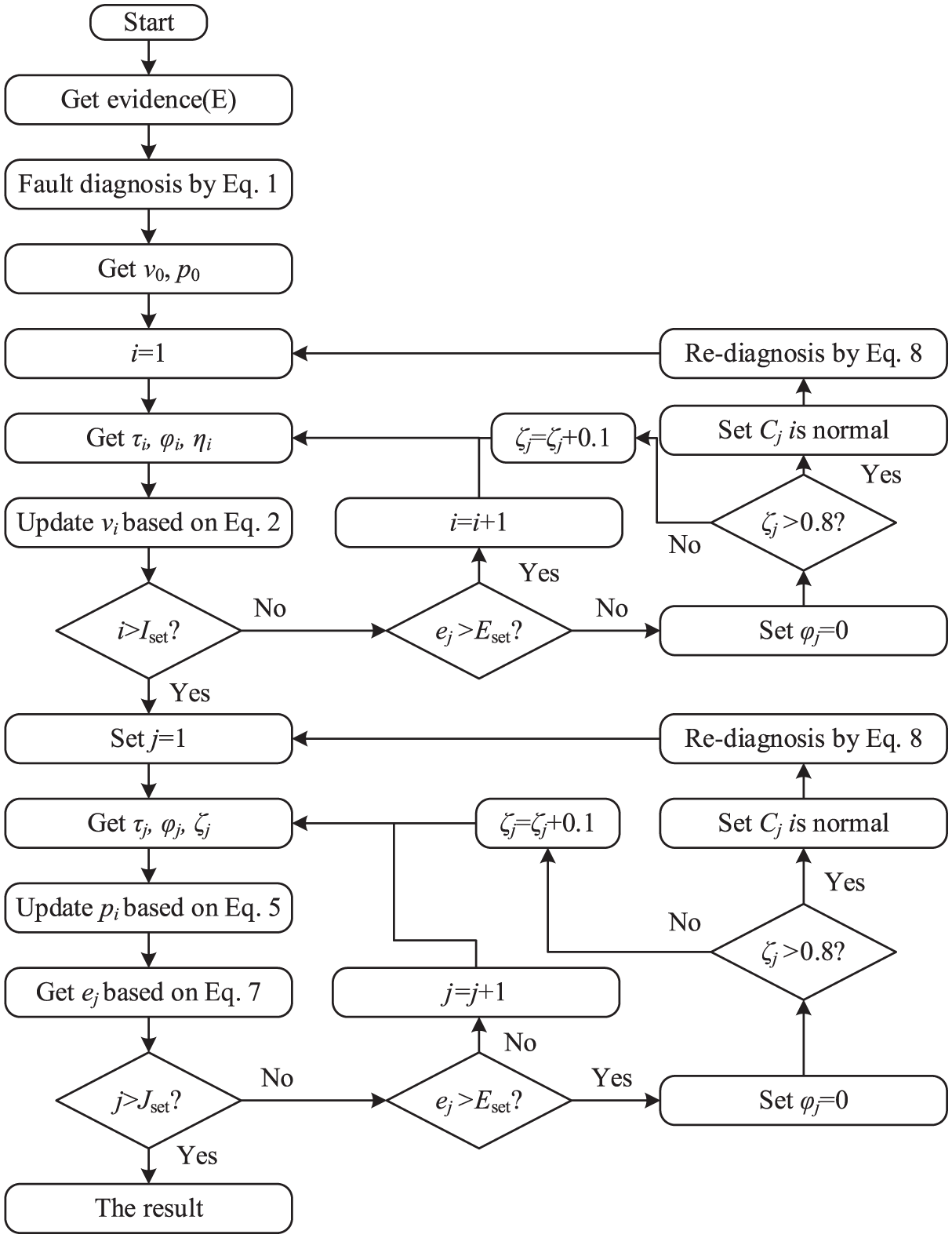
The fault diagnosis process.

Case study: A hydraulic system with multiple control flows

The introduction of the system

A hydraulic system with multiple control flows, shown in Figure 3, is used as a case study. This system is composed of three primary modules: the power module, the control module, and the hydraulic module. The power module includes components such as transformers and motor frequency converters, and it serves to supply the necessary power for the system. The control module consists of components such as PLCs, switches, and optocouplers, and is responsible for managing the operation of the system. The hydraulic module contains hydraulic components and functions as the main execution module.

Figure 3.

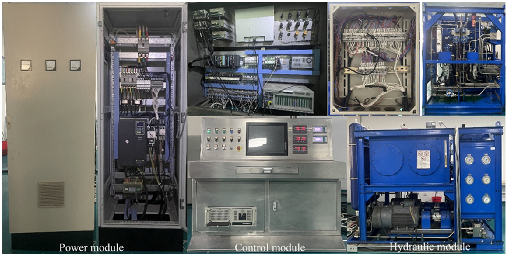
The hydraulic system with multiple control flows.

The system’s control schematic is presented in Figure 4. The function of the system is to provide hydraulic power for subsea oil and gas equipment. To ensure sufficient pressure supply, two pumps were used. A butterfly valve (BV) at the fuel tank outlet regulates the supply of hydraulic oil, while a motor drives the pumps to supply power to the circuit. The BV is manually controlled. An overflow valve is installed at the pump outlet to control the circuit’s overall pressure. In each circuit, a manual valve, a pressure maintaining valve, and a pressure sensor are installed. They are used to ensure stable export pressure and visibility. The system includes four outlets, which distribute hydraulic power to other actuators. Additionally, a directional valve (DT2 in Figure 4) manages the operation of the accumulator. When activated, the accumulator ensures pressure stability within the system, even during pump inactivity.

Figure 4.

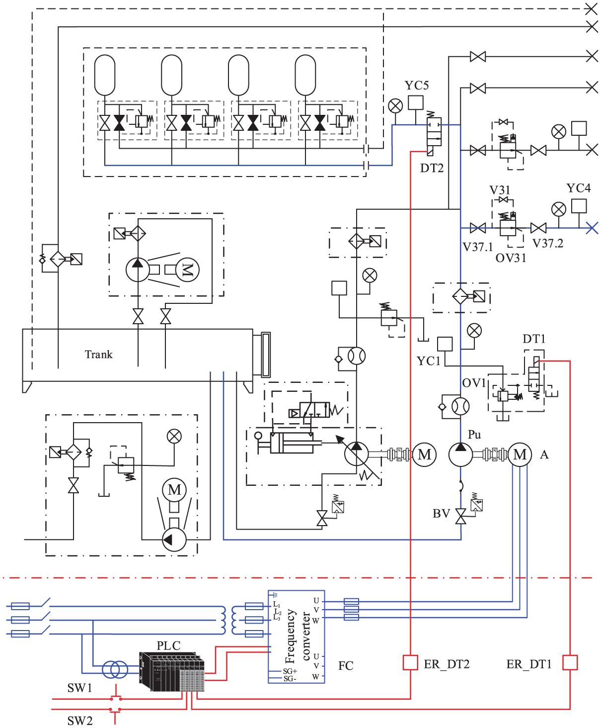
The drawing of the hydraulic system with multiple control flows.

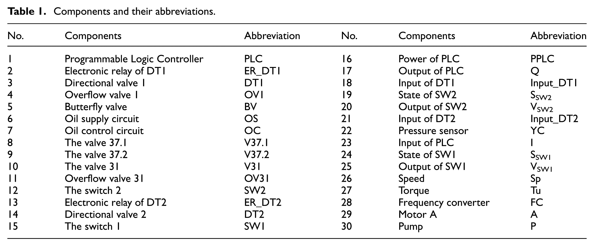
All hydraulic components are controlled by a PLC within the control module. The PLC also monitors data from hydraulic sensors, torque sensors, and speed sensors. A configuration software running on a PC is connected to the PLC for data acquisition and system control. The blue circuit and its associated components in Figure 5 are utilized for the case study. A comprehensive list of component and sensor abbreviations is provided in Table 1. The data required in this case was also collected and obtained from the PLC.

Figure 5.

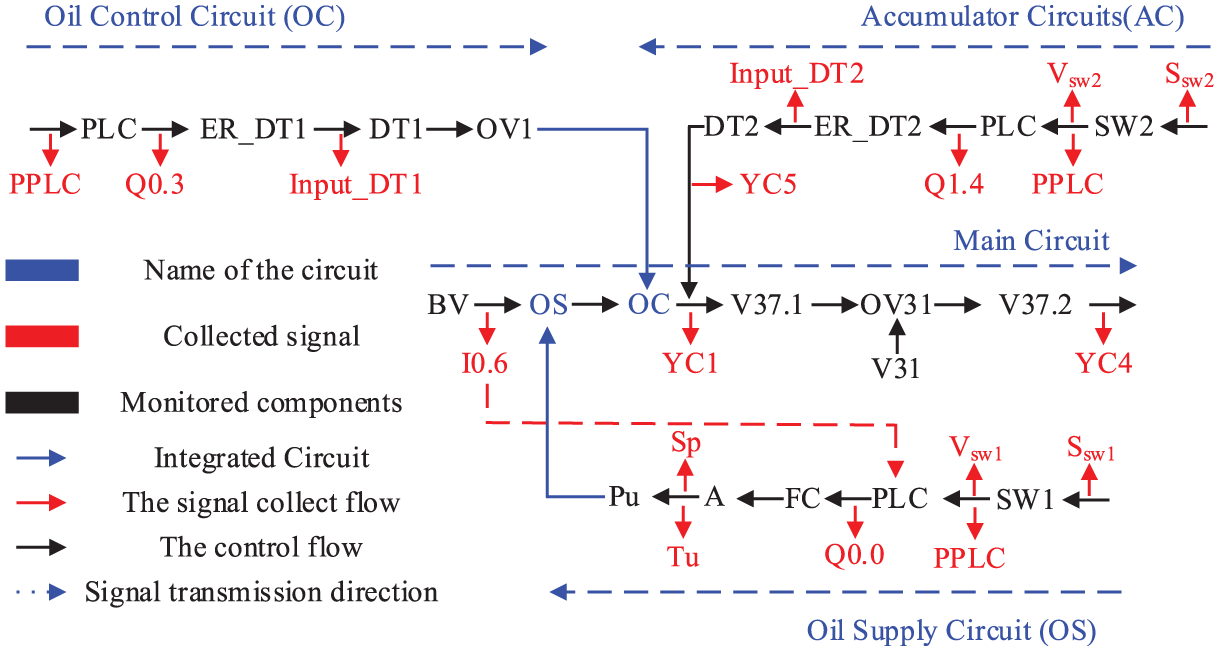
The control flow of the studied circuit.

Table 1.

Components and their abbreviations.

No.	Components	Abbreviation	No.	Components	Abbreviation
1	Programmable Logic Controller	PLC	16	Power of PLC	PPLC
2	Electronic relay of DT1	ER_DT1	17	Output of PLC	Q
3	Directional valve 1	DT1	18	Input of DT1	Input_DT1
4	Overflow valve 1	OV1	19	State of SW2	S_SW2
5	Butterfly valve	BV	20	Output of SW2	V_SW2
6	Oil supply circuit	OS	21	Input of DT2	Input_DT2
7	Oil control circuit	OC	22	Pressure sensor	YC
8	The valve 37.1	V37.1	23	Input of PLC	I
9	The valve 37.2	V37.2	24	State of SW1	S_SW1
10	The valve 31	V31	25	Output of SW1	V_SW1
11	Overflow valve 31	OV31	26	Speed	Sp
12	The switch 2	SW2	27	Torque	Tu
13	Electronic relay of DT2	ER_DT2	28	Frequency converter	FC
14	Directional valve 2	DT2	29	Motor A	A
15	The switch 1	SW1	30	Pump	P

Faults that cause the same consequences can be grouped together by the grouping method based on the control flow. In this case, the fault diagnosis model can ignore their similar results. For example, unopened valves, pressure changes, etc. The model focuses more on the different fault characteristics, which makes it easier to distinguish fault types. The control flow of the hydraulic circuit is illustrated in Figure 5, where all available monitoring data are also presented. When selecting the collected signals, signals related to the diagnosed component were chosen. This is because irrelevant signals would increase modeling costs. In addition, they can interfere with the diagnostic results.

The circuit is divided into four distinct control sections: the main circuit, the oil supply circuit, the oil control circuit, and the accumulator circuit. The main circuit consists primarily of valves and pumps, which are responsible for controlling the flow of hydraulic oil. The primary sensor data monitored within this circuit include pressure readings, which are crucial for ensuring stable operation. The oil supply circuit, on the other hand, is designed to control the motor, with its key components comprising buttons, a PLC, a frequency converter, and the motor itself. The measurable parameters in this circuit include the output voltage of the PLC, as well as motor speed and torque.

In the remaining two circuits—the oil control and accumulator circuits—the directional valve is managed by the PLC. The primary components in these circuits include the PLC, electronic relays, and the controlled valve. The monitoring data in these circuits consist exclusively of voltage measurements at critical points, which provide insights into the operational status and effectiveness of control.

Fault setting

The four control parts are configured with different fault conditions, and the methods for setting these faults are described as follows:

The faults in the main circuit are illustrated in Figure 6. One fault involves the blockage of sediment in the tank, which affects the BV. This fault can lead to an insufficient supply of hydraulic oil. In the experiment, this condition is simulated by adjusting the opening and closing degree of the BV. As depicted in Figure 6, various closing degrees are implemented separately to replicate the fault scenario. Notably, during fault simulation, the position sensor of the BV continues to provide normal signals. Consequently, the PLC receives this normal information and operates the motor without detecting any anomalies in the BV.

Figure 6.

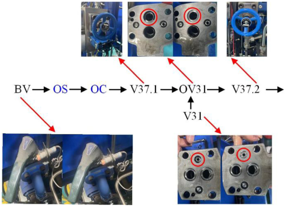
The fault set in the main circuit.

For the manual valves V37.1 and V37.2, faults are introduced by varying their opening and closing degrees. This adjustment mimics conditions where the valves deviate from their intended operational positions. In the case of the overflow valve (OV), the failure mode is characterized as leakage. To replicate this fault, different degrees of leakage are introduced for OV31 and V312 by intentionally damaging their gaskets. These settings allow for a controlled study of the system’s response to varying fault levels.

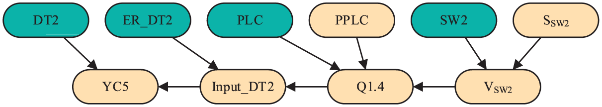
The fault settings in the accumulator circuit are depicted in Figure 7. For the directional valve DT2, three different levels of leakage are introduced by intentionally damaging the gasket. These varying degrees of leakage allow for a detailed analysis of the system’s behavior under different fault severities. To simulate signal loss for SW2, two scenarios are configured: first, by unplugging the output terminal of SW2, and second, by disconnecting its input section from the PLC. These conditions replicate the potential failure modes where SW2 is unable to communicate effectively with the PLC. Fault simulation for the PLC involves disconnecting its output, thereby preventing downstream circuits from receiving the necessary control signals. Similarly, the fault condition for the electronic relay ER_DT2 is replicated by interrupting its output, simulating a failure in its operation.

Figure 7.

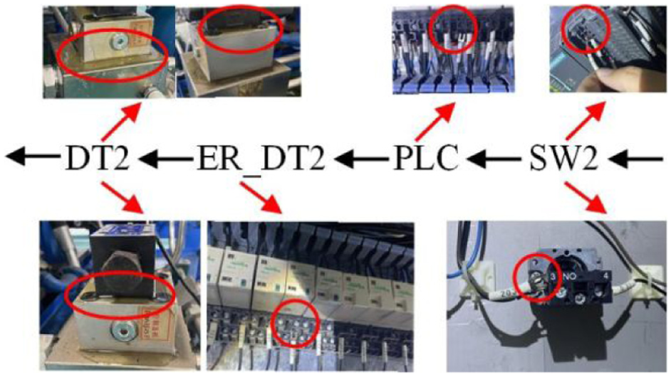
The fault set in the accumulator circuit.

The fault settings in the oil control circuit are illustrated in Figure 8. For DT1 and OV1, faults are simulated by introducing varying degrees of damage to their gaskets, thereby replicating different levels of malfunction.^27,28 These controlled fault conditions enable an in-depth evaluation of the circuit’s performance under varying operational constraints.

Figure 8.

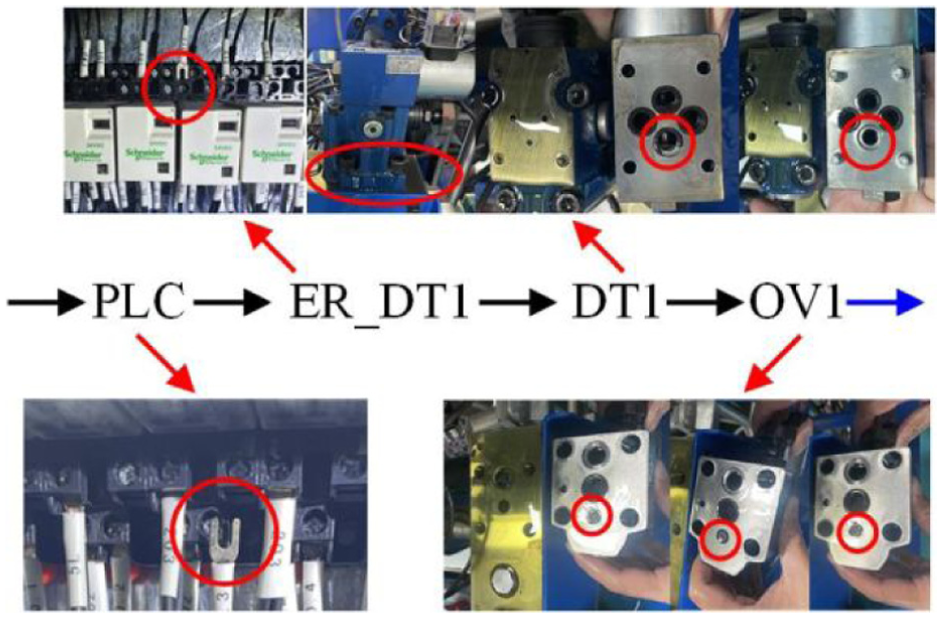
The fault set in the oil control circuit.

To simulate faults in the PLC and ER_DT1, their outputs are deliberately disconnected. This interruption prevents subsequent components from receiving control signals, effectively mimicking failure scenarios in these critical elements. These fault settings are essential for analyzing the robustness and fault-tolerance of the oil control circuit under different failure modes.

The fault settings in the oil supply circuit are presented in Figure 9. Faults in this circuit are primarily simulated by disconnecting components to replicate various failure conditions. Additionally, PLC faults are introduced by disconnecting the power supply to specific racks, thereby preventing their operation and simulating control failures.

Figure 9.

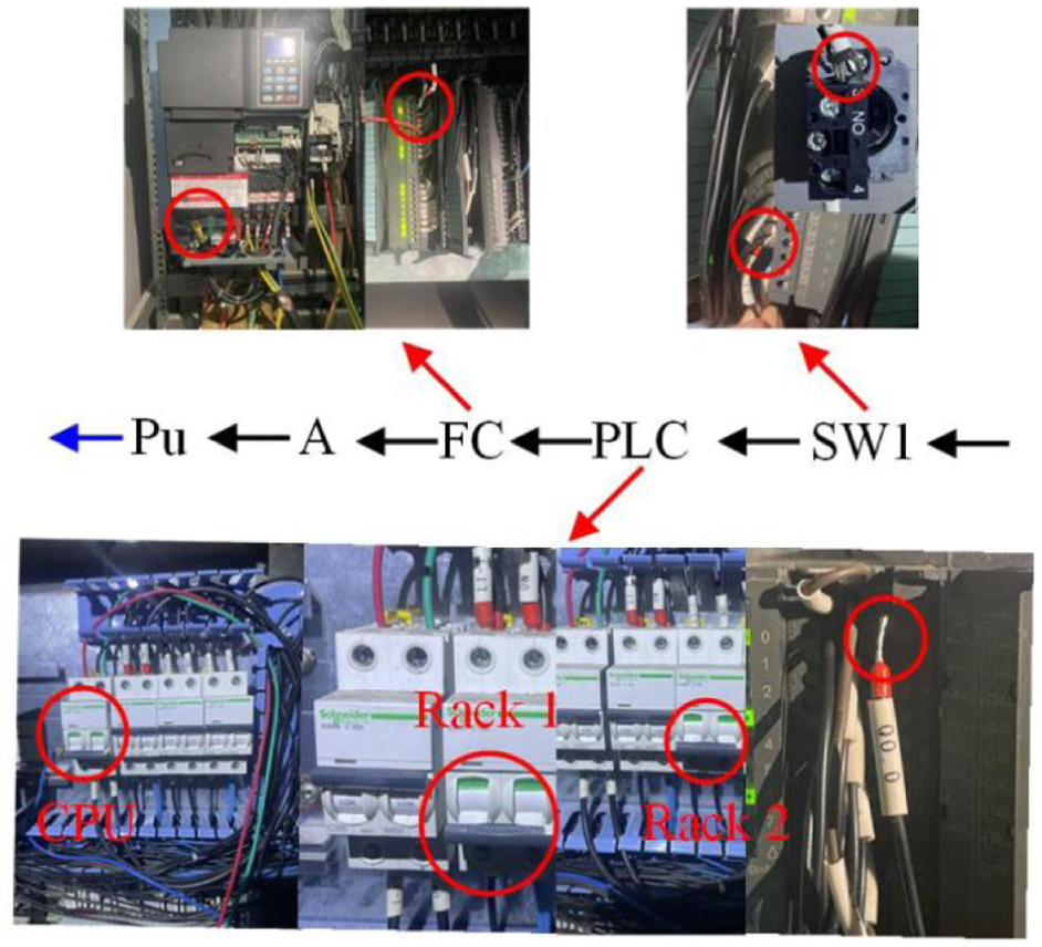
The fault set in the oil supply circuit.

It is important to note that faults in components A and Pu are not simulated due to safety concerns associated with their operation. This precaution ensures that the fault simulation process does not compromise the safety of the system or its operators.

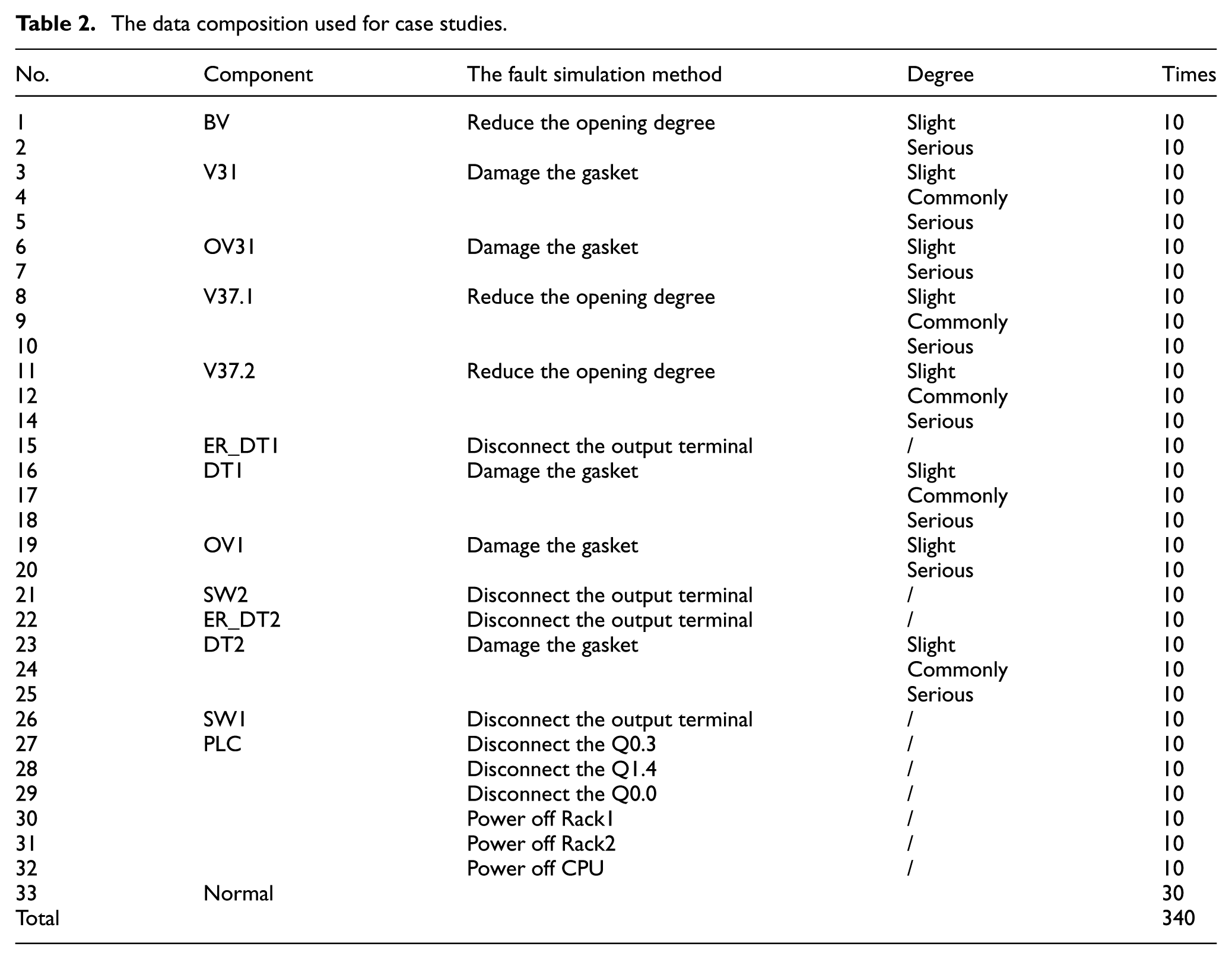
To ensure the reliability of the results and avoid accidental outcomes, each fault scenario is simulated multiple times. The number of simulations conducted for each fault type is detailed in Table 2, which also represents the dataset used for the case study analysis.

Table 2.

The data composition used for case studies.

No.	Component	The fault simulation method	Degree	Times
1	BV	Reduce the opening degree	Slight	10
2	BV	Reduce the opening degree	Serious	10
3	V31	Damage the gasket	Slight	10
4			Commonly	10
5			Serious	10
6	OV31	Damage the gasket	Slight	10
7	OV31	Damage the gasket	Serious	10
8	V37.1	Reduce the opening degree	Slight	10
9			Commonly	10
10			Serious	10
11	V37.2	Reduce the opening degree	Slight	10
12			Commonly	10
14			Serious	10
15	ER_DT1	Disconnect the output terminal	/	10
16	DT1	Damage the gasket	Slight	10
17			Commonly	10
18			Serious	10
19	OV1	Damage the gasket	Slight	10
20	OV1	Damage the gasket	Serious	10
21	SW2	Disconnect the output terminal	/	10
22	ER_DT2	Disconnect the output terminal	/	10
23	DT2	Damage the gasket	Slight	10
24			Commonly	10
25			Serious	10
26	SW1	Disconnect the output terminal	/	10
27	PLC	Disconnect the Q0.3	/	10
28		Disconnect the Q1.4	/	10
29		Disconnect the Q0.0	/	10
30		Power off Rack1	/	10
31		Power off Rack2	/	10
32		Power off CPU	/	10
33	Normal			30
Total				340

The fault diagnosis model

The fault diagnosis model of the operating system (OS) is depicted in Figure 10. The network consists of three types of nodes: monitored nodes, state nodes, and symptom nodes.

Figure 10.

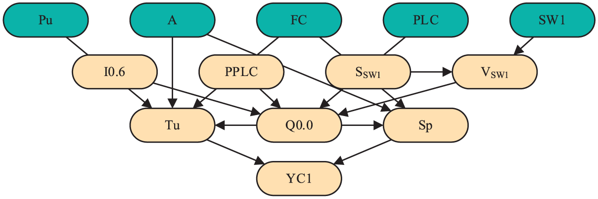
The fault diagnosis model of the OS.

Monitored nodes represent the components that must be observed within the system. In this circuit, the monitored nodes include Pu, A, FC, PLC, and SW1, as these components directly influence the system’s behavior. Therefore, they are designated as parent nodes.

State nodes correspond to the conditions of the monitored nodes. For instance, in this circuit, S_sw1 is a state node representing the status of SW1. If SW1 is open, the state of S_sw1 is 1; otherwise, it is 0. This information can be retrieved from the control module. The state of SW1 also impacts the output of the PLC, making it a parent node for Q0.0.

The remaining nodes are symptom nodes, which provide evidence of faults and are collected via sensors and the PLC. These nodes act as child nodes within the model. During the fault diagnosis process, evidence gathered from the sensors and PLC is used to update the symptom and state nodes. Based on this information, the faults of the monitored nodes are inferred.

In the re-diagnosis process, some monitored nodes are assumed to be functioning normally, while others are re-evaluated for faults. It is important to note that the monitored nodes can have two possible states: normal and abnormal. Regardless of the severity of the malfunction, any deviation from normal operation is considered abnormal. The degree of faults in the monitored nodes can be determined through the algorithm outlined in Table 2.

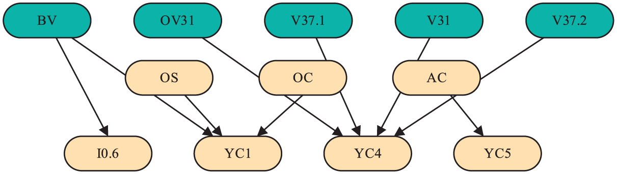
The fault diagnosis model of the OC is shown in Figure 11. The ER_DT1 and PLC can be monitored by the only fault symptom. The state of the OV1 and DT1 should be monitored by common fault symptom.

Figure 11.

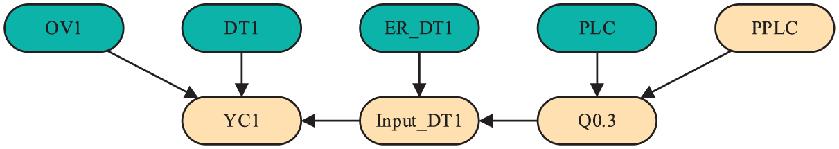
The fault diagnosis model of the OC.

The fault diagnosis model of the AC is shown in Figure 12. In this model, all monitored nodes are diagnosed through a single indicator. The SSW2 are used to avoid misdiagnosis caused by control. The PPLC is used to monitor the power of the PLC.

Figure 12.

The fault diagnosis model of the AC.

The fault diagnosis model of the main circuit is illustrated in Figure 13. Unlike the previous model, three additional nodes, OS, OC, and AC are incorporated. These nodes represent three other control flows, the faults of which can influence the performance of the main circuit. As a result, they are added as parent nodes in the model. When components within these three circuits fail, the corresponding node status is set to “fault.” The probability tables for all models are derived through expert decision-making, ensuring the accuracy and reliability of the fault diagnosis process.

Figure 13.

The fault diagnosis model of the main circuit.

For comparison, a larger model without grouping is established, as shown in Figure 14. The relationships of the nodes remain consistent with those in the grouped model, with the main difference being that some nodes are merged. For example, the PLC, PPLC, and YC1 nodes are combined into single entities in this model. Similarly, the re-diagnosis process based on digital twin models is also incorporated into this larger model. It should be pointed out that the parent-child relationship in this model is established based on their correlation. All diagnosed components only establish parent-child relationships with the signals related to them, which prevents unnecessary causal relationships from affecting the diagnostic results.

Figure 14.

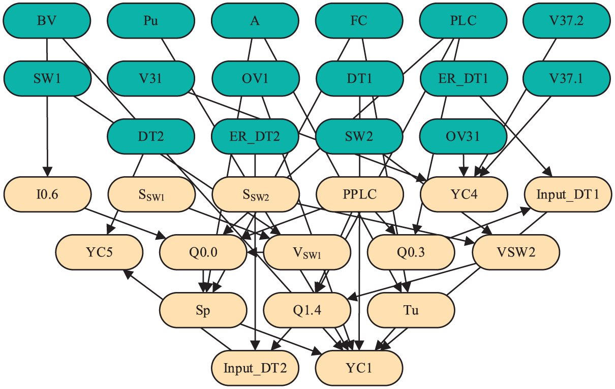
Fault diagnosis model for comparison.

The results and discussion

The accuracy of fault diagnosis for different components is shown in Figure 15. The results illustrate the diagnostic performance of the two models and highlight the improvements introduced by the digital twin model. Specifically, the results demonstrate that the accuracy of fault diagnosis ranges between 85% and 87% when the group fault diagnosis method is not applied. However, when the group fault diagnosis method is utilized, the accuracy improves significantly, leading to better fault detection and diagnosis performance.

Figure 15.

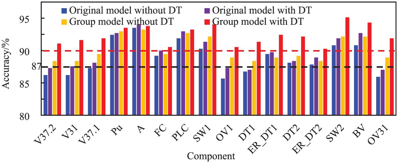
The accuracy of fault diagnosis for different components.

When the group fault diagnosis method is applied, the accuracy of fault diagnosis increases slightly to above 87.5%, representing an improvement of nearly 2.5%. This indicates that the group fault diagnosis method effectively isolates interference information, thereby enhancing overall performance. From the perspective of the digital twin, performance is further improved when the digital twin model is integrated, consistent with findings from existing research.²⁵ Interestingly, the degree of improvement varies between the two models. For the model without the group fault diagnosis method, the integration of the digital twin model results in a 5% improvement in diagnostic accuracy. In contrast, when the group fault diagnosis method is used, this improvement rises to approximately 10%. This suggests that the group fault diagnosis method enhances the utilization of feedback information.

The overall accuracy of the fault diagnosis is shown in Figure 16. The diagnostic accuracy of the proposed model reached 92.36%. Compared to that, the increase is about 5%. From the results, it is evident that the group fault diagnosis method enhances the accuracy of fault diagnosis. As shown in Figure 15, this improvement is primarily due to the ability of the method to better recognize faults with similar symptoms. Additionally, the digital twin model contributes to an increase in diagnostic accuracy. However, it is important to note that the overall improvement in diagnostic results due to the digital twin model is not substantial. This is because the diagnostic accuracy for certain components is already very high, so the impact of the digital twin model is less pronounced, resulting in a smaller overall improvement.

Figure 16.

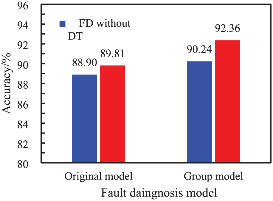
The overall accuracy.

The accuracy for each circuit is presented in Figure 17. It is evident that the main circuit exhibits the lowest accuracy, primarily due to the limited number of sensors in this circuit. When the group fault diagnosis method is applied, the diagnostic accuracy across the four circuits becomes more similar. Among these, the accuracy for the oil supply circuit is the highest. This can be attributed to two factors: First, each component in this circuit has distinct information for monitoring its status, which facilitates easier identification of faults. Second, since faults are set for Pu and A, their high accuracy contributes to an overall improvement in the average diagnostic accuracy.

Figure 17.

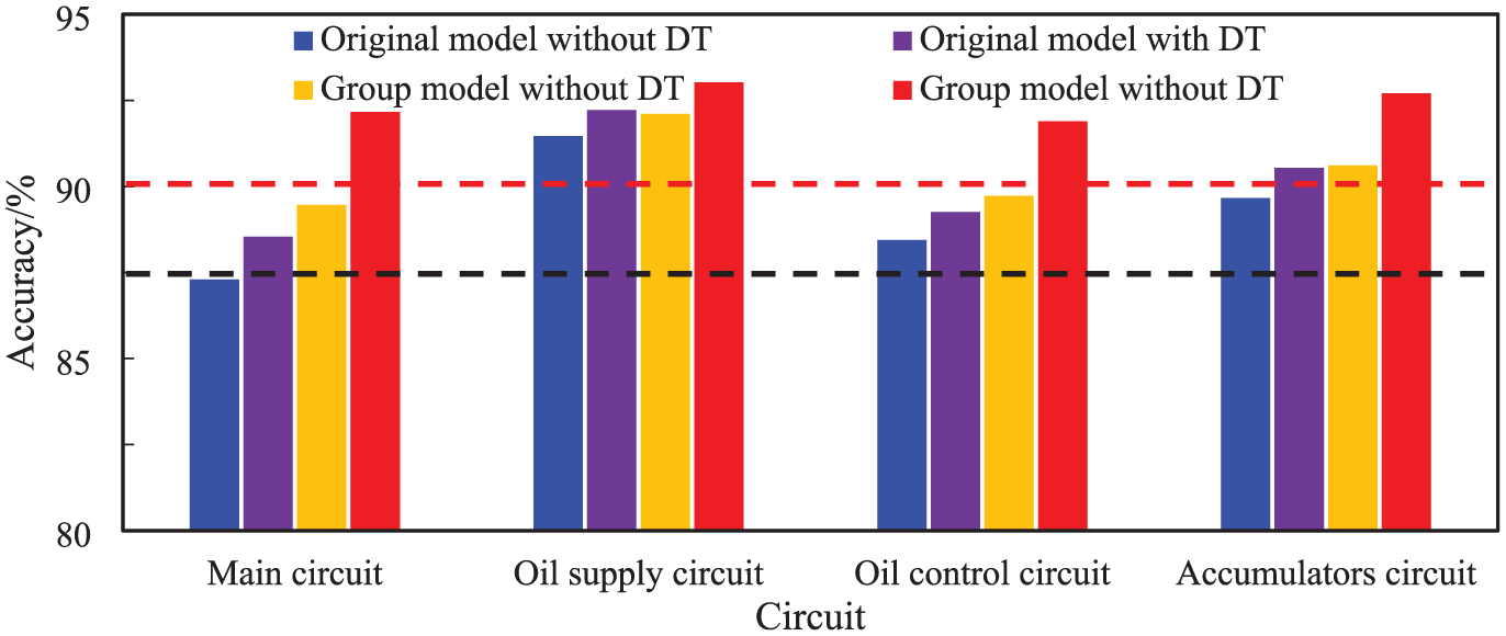
The accuracy for each control flow.

To investigate the relationship between information and the accuracy of fault diagnosis, a “degree of information” is defined in this study. The degree of information is quantified as the number of sensors that can be influenced by the fault of a given component. If a sensor is affected by the failure of multiple components, the contribution of each component to the sensor is considered equal. The calculation method for the degree of information is as follows:

DI = S + \sum_{1}^{S_{n}} \frac{1}{n_{i}}

(9)

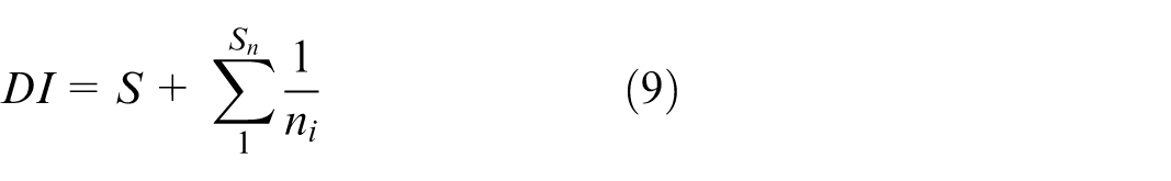
where, DI is the degree of information, S is the number of sensors that is only influenced by the certain component, S_n is the number of sensors that is influenced by the several components, n_i is the number of the components that influence the same sensor.

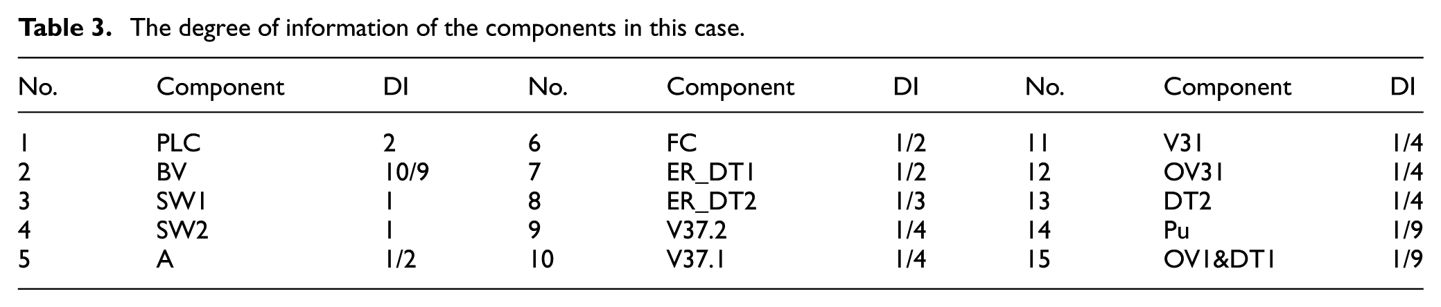
The degree of information of the components in this case is given in Table 3.

Table 3.

The degree of information of the components in this case.

No.	Component	DI	No.	Component	DI	No.	Component	DI
1	PLC	2	6	FC	1/2	11	V31	1/4
2	BV	10/9	7	ER_DT1	1/2	12	OV31	1/4
3	SW1	1	8	ER_DT2	1/3	13	DT2	1/4
4	SW2	1	9	V37.2	1/4	14	Pu	1/9
5	A	1/2	10	V37.1	1/4	15	OV1&DT1	1/9

The relationship between accuracy and the degree of information is shown in Figure 18. The accuracy at each degree of information is calculated by averaging the accuracy of all components with that particular degree of information. Overall, a positive correlation is observed between accuracy and the degree of information. This pattern is consistent across both models, even without re-diagnosis. Compared to the original models, the group fault diagnosis method demonstrates higher accuracy at every degree of information, especially when the degree of information is low.

Figure 18.

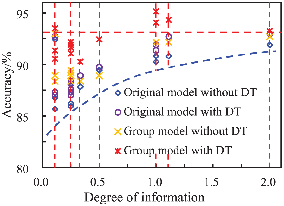
The relationship between the accuracy and the degree of information.

However, when the combination of re-diagnosis with the digital twin model is applied, a different trend emerges. Accuracy is higher near a degree of information of 1, but decreases as the degree of information approaches 2. This is because the verification process relies on judging the output error, and more judgment information typically introduces more error parameters. This can result in larger errors, which impact the overall average error and lead to misjudgments. Despite this, the combination of re-diagnosis with the digital twin model still significantly enhances the accuracy at every degree of information.

Conclusion

A digital twin-driven group fault diagnosis method is proposed for fault diagnosis of faults with similar features. A re-diagnosis mechanism based on the DTM was proposed. The single diagnosis process becomes a multiple re-diagnosis process. A grouping diagnosis method based on control flow was proposed. Similar faults are grouped for diagnosis. A hydraulic power unit was used to study the performance of this method. The faults of each component have been simulated. The results show that the group fault diagnosis method improves the accuracy of the fault diagnosis. The accuracy increases by 3%–5% compared to the original fault diagnosis model. Furthermore, the integration of the digital twin model significantly aids in fault identification, enhancing diagnostic accuracy. Compared to one-time fault diagnosis, the re-diagnosis method utilizing the digital twin model improves accuracy by nearly 10%. Additionally, a positive correlation between accuracy and the degree of information is observed, with the re-diagnosis method achieving higher accuracy at the same degree of information. These findings demonstrate that both the group fault diagnosis method and the digital twin model play crucial roles in improving the reliability and precision of fault diagnosis in complex systems.

This method effectively solves the problem of diagnose similar faults. Currently, the performance has only been validated on a single case in the laboratory. Expanding the applicability and proving its suitability in different scenarios would be a future research direction. In addition, quantification of fault severity is an important research direction for fault diagnosis. The faults in this research are all achieved by setting different levels of leakage and blockage. The quantification of fault severity setting methods is an important future research direction. What’s more, improving diagnostic efficiency and reducing diagnostic time are also important research directions.

Footnotes

ORCID iD

Chao Yang

Ethical considerations

I commit to conducting myself with integrity and honesty, respecting intellectual property and confidentiality, and ensuring fairness and objectivity in all my work.

Consent to participate

This article does not contain any studies with human or animal participants.

Consent for publication

All authors have read and approved the final manuscript and consent to its publication.

Funding

The authors disclosed receipt of the following financial support for the research, authorship, and/or publication of this article: This work was supported by the National Natural Science Foundation of China (No. 52325107), High tech Ship Research Project of Ministry of Industry and Information Technology (No. 2023GXB01-05-004-03, No. GXBZH2022-293), the National Science and Technology Major Project of China (2025ZD1403501-05), and the Fundamental Research Funds for the Central Universities (No. 24CX10006A).

Declaration of conflicting interests

The authors declared no potential conflicts of interest with respect to the research, authorship, and/or publication of this article.

Data availability statement

The datasets generated and/or analyzed during the current study are available from the corresponding author on reasonable request. Digital Twin Driven Group Fault Diagnosis Method for Faults with Similar Symptoms.

References

Zhang

Zhou

Meng

, et al. Steady-state fault propagation characteristics and fault isolation in cascade electro-hydraulic control system. Machines 2024; 12(9): 600.

Zhao

Zio

Shen

. Domain generalization for cross-domain fault diagnosis: an application-oriented perspective and a benchmark study. Reliab Eng Syst Saf 2024; 245: 109964.

Liu

Dang

Lee

. Research on the protection system for smart grid based on phasor information at circuit breakers. Energies 2024; 17(14): 3455.

Shao

Cai

. System-level remaining useful life prediction methodology based on the dynamic health index of multi-indicator fusion: two cases of subsea equipment. J Ocean Eng Sci 2026. https://doi.org/10.1016/j.joes.2026.01.003

Wang

Tian

Yang

, et al. Neural-transformer: a brain-inspired lightweight mechanical fault diagnosis method under noise. Reliab Eng Syst Saf 2024; 251: 110409.

Rastogi

Shah

Singh

, et al. Mode analysis, transformer saturation, and fault diagnosis technique for an open-circuit fault in a three-phase DAB converter. IEEE Trans Power Electron 2023; 38(6): 7644–7660.

Rastogi

Shah

Singh

, et al. Vector-based open-circuit fault diagnosis technique for a three-phase DAB converter. IEEE Trans Ind Electron 2024; 71(7): 8207–8211.

Zhang

Song

Wang

, et al. High-resistance connection fault diagnosis of srm based on multisensor calibrated transformer with shifted windows. IEEE Sens J 2023; 23(24): 30971–30983.

Prabhakaran

Thirumoorthi

Sri Dhivya Krishnan

. Design and development of an intelligent zone based master electronic control unit for power optimization in electric vehicles. Sci Rep 2024; 14(1): 20142.

10.

Gan

Ding

Qiu

, et al. Model-based safety analysis with time resolution (MBSA-TR) method for complex aerothermal–mechanical systems of aero-engines. Reliab Eng Syst Saf 2024; 243: 109864.

11.

Zhang

Rangaiah

Dong

, et al. A novel fault diagnosis framework for industrial production processes based on causal network inference. Ind Eng Chem Res 2024; 63: 9471–9488.

12.

Liu

Peng

, et al. Reliable composite fault diagnosis of hydraulic systems based on linear discriminant analysis and multi-output hybrid kernel extreme learning machine. Reliab Eng Syst Saf 2023; 234: 109178.

13.

Wang

Zhang

, et al. Metric-based meta-learning model for few-shot fault diagnosis under multiple limited data conditions. Mech Syst Signal Process 2021; 155: 107510.

14.

Gao

Wang

Zhang

, et al. Hybrid fault diagnosis method for underwater thrusters based on the common features of multi-source signals. Mech Syst Signal Process 2025; 222: 111740.

15.

Guo

. Active fault diagnosis for stochastic systems under accuracy-limited sensors. IEEE Trans Instrum Meas 2024; 73: 1–9.

16.

Zhang

Liang

Zhao

, et al. Electro-hydraulic SBW fault diagnosis method based on novel 1DCNN-LSTM with attention mechanisms and transfer learning. Mech Syst Signal Process 2024; 220: 111644.

17.

Yang

Cai

Kong

, et al. A digital twin-assisted intelligent fault diagnosis method for hydraulic systems. J Ind Inf Integr 2024; 42: 100725.

18.

Xia

Huang

, et al. Digital twin-assisted fault diagnosis of rotating machinery without measured fault data. IEEE Trans Instrum Meas 2024; 73: 1–10.

19.

Jmal

Naifar

Ben Makhlouf

, et al. Fault tolerant control for linear fractional order systems with sensor faults. In: 2018 15th international multi-conference on systems, signals and devices (SSD), 2018, pp.105–110.

20.

Huang

Xie

Luo

, et al. Incremental learning with multi-fidelity information fusion for digital twin-driven bearing fault diagnosis. Eng Appl Artif Intell 2024; 133(B): 108212.

21.

Jing

Liu

, et al. Research on digital technology of mechanical structure fault diagnosis of power transformer based on comprehensive feature extraction and SABO-PNN. IEEE Trans Appl Supercond 2024; 34(8): 1–4.

22.

Liu

Lang

Gui

, et al. Digital twin-based anomaly detection for real-time tool condition monitoring in machining. J Manuf Syst 2024; 75: 163–173.

23.

Yang

Cai

Zhang

, et al. Cross-validation enhanced digital twin driven fault diagnosis methodology for minor faults of subsea production control system. Mech Syst Signal Process 2023; 204: 110813.

24.

Yang

Cai

Liu

, et al. Intelligent full-stage stable fault diagnosis method for subsea production system. Ocean Eng 2024; 312(3): 119309.

25.

Kong

Cai

Khan

, et al. Concurrent fault diagnosis method for electric-hydraulic system: subsea blowout preventer system as a case study. Ocean Eng 2024; 294: 116818.

26.

Yang

Cai

, et al. Digital twin-driven fault diagnosis method for composite faults by combining virtual and real data. J Ind Inf Integr 2023; 33: 100469.

27.

Dhouibi

Sakly

Sethom

HBA

. A novel fuzzy nonlinear PID controller design for underactuated rotary inverted pendulum system: simulation and real-time implementation. In: Proceedings of the 2022 17th international conference on control, automation, robotics and vision (ICARCV), 2022, pp.402–407. IEEE.

28.

Serral

Valderas

Pastor

. On the modeling of collaborative and multi-modal processes. In: Research challenges in information science. Lecture notes in business information processing. Vol 385. Springer, 2020, pp.95–111.