
Abstract
To improve product qualities and obtain maximum comprehensive economic benefits from batch process production, it is of great practical significance to optimize the operation of batch production processes. Considering the multiphase and slow time-varying characteristics, a multiphase time-varying batch process monitoring method is proposed based on stage moving model migration technology. Firstly, the sliding windows are constructed with moving phases, where the moving of different phases is decided by the influence of the process variables to the final product. And time slices are the basic units for building the regression models. Secondly, to analyze and capture the relationship between the process variables of both the old mode and new mode and the final quality variable, the JY-PLS algorithm is utilized on each time slice within sliding windows for quality prediction. Then, monitoring indexes and corresponding control limits are calculated and used for process monitoring. The application to a real multiphase time-varying batch process, the start-up process of injection molding process, proved the effectiveness of the proposed method.
Introduction
To improve the ability to meet the needs of the changing market situation, batch and half-batch processes play an increasingly important role in many industrial production industries. They are especially applicable in the production and processing of high-quality and high-value-added specialty chemicals (such as polymers, pharmaceuticals, biological chemicals, food, semiconductors and agricultural chemicals). People’s demand for high quality products is also increasing with the increasingly fierce international competition. Therefore, the model establishment, online monitoring and fault diagnosis of the batch process are of great significance.
The batch process is implemented by accurately ordering and automating all phases of the sequence, converting the raw material into a product for a limited duration. From an engineering perspective, the goal of the batch processing process is to achieve product production of consistent and reproducible quality in the batch process design on a competitive price basis. Usually, the batch process presents multiphase characteristics due to the needs of different operations. At the same time, the batch process always exhibits some batch-to-batch variation on its trajectory, that is, the slow time-varying characteristic. Quality control during the batch process enables the product to achieve a uniform quality. The batch process usually shows time-varying, dynamic, and non-linear characteristics. To improve the quality of the batch process products and enhance the safety of the production process, it is necessary to establish the quality prediction system model and monitor the process through the online fault monitoring system.
At present, in the analysis of batch process, most researchers choose to use the analysis techniques in multivariate statistical analysis, such as principal element analysis (PCA),1,2 partial least squares regression (PLS),3,4 independent component analysis (ICA), 5 etc. Among the above methods, PLS is well used for many problems, so it is widely used at present. In the mid-1990s, Nomikos and MacGregor 3 first successfully introduced multivariate statistics into the batch process for research and analysis. Subsequently, Zarzo and Ferrer 6 used the PLS algorithm to analyze the data of the batch chemical process, and successfully diagnosed the reasons for the change in the final quality parameters. García Muñoz et al. 7 proposed a mass Joint latent variable partial least squares model (JY-PLS) and model inversion method to obtain a preliminary solution based on the existing historical database for product transfer. JY-PLS selects all variables of the old and new processes to extract data features, thus establishing regression models of hidden variables and obtaining public space information for model migration. In addition, Li et al. 8 realized the application of near infrared spectrum in the monitoring of batch cooling crystallization process by using genetic algorithm and PLS, and focused on the wavelength selection of applying genetic algorithm in the development of PLS calibration model. Shan et al. 9 proposed a mixed model of partial least squares-slice transformation based on nonlinear calibration of partial least squares and slice transformation for simulating nonlinear chemical systems with a wide range of response variables. Gomes Ade et al. proposed a combination of PLS noise reduction characteristics and no information variables discard in SPA new algorithm. 10 Ringle et al. put forward the PLS genetic algorithm segmentation (PLS-GAS) method to explain the not observed heterogeneity in path model estimation and guide the evaluation of the new method through the simulation results. 11 Allegrini and Olivieri proposed a new method to estimate the detection limit problem in PLS calibration. 12
In the industrial batch process production, the production of products with specified specifications is the main goal and a challenge in the batch process production. A major technical and economic goal in industry is the reproducibility of the final product composition. Due to the complexity and unforeseen interference of the batch process industry, such as equipment failure, changes in raw material performance and the instability of the process operating conditions, product quality may be seriously different from the specifications, possibly producing the final product that meets the specifications. If a quality prediction model can be established in the batch production process to predict the output quality for subsequent batches, so that the corresponding process conditions can be adjusted in advance and the products can meet the expected specifications, which is very important industrial production significance. The success and performance of real-time quality control depends on the availability and accuracy of the model. How to develop a model that describes the underlying relationship based on available process measurements and how to accurately describe this relationship by extracting appropriate information from multivariate process data are challenges in model development and key to process quality control.
Under normal circumstances, the method of quality prediction is divided into two categories: the first is the prediction method based on the mechanism model of industrial process, mainly through the in-depth analysis of the industrial process, the application of physical and chemical principle knowledge of the entire reaction process, and the reaction equation in the production process (such as thermodynamic equations, chemical reaction equations, etc.) to build a precise and accurate mechanism model. The advantage of such methods is accuracy. For industrial processes with relatively simple reaction processes, the final mass can be accurately predicted by establishing mechanism models. However, industrial processes with a higher degree of complexity usually have strong nonlinear, time-varying, and no fixed steady-state operating point, which makes it very difficult to establish the mechanism model of industrial processes. Therefore, in the industrial batch processes, the application conditions of the mechanism model are relatively strict, and cannot be extended to a wide range of industrial processes for use. Therefore, the second method is usually used in modern industrial batch process production, prediction based on batch process data modeling. This kind of method mainly samples and records the process variable data in batch process production as input, and takes the final quality variable as output. Based on multivariate statistics method, a mathematical model between the input and output is established, so that the output quality of subsequent batches can be predicted by using the collected process data of new batches. Compared with the previous one, this method is more concise in modeling process and requires less knowledge of the reaction mechanism of industrial process, so it has been favored by researchers.
Effective monitoring and control of batch processes is essential to produce high-quality materials. The batch process is characterized by the processing of raw materials into products in a limited amount of time, and the main goal is to continuously produce products of the required quality at the lowest possible cost. However, small changes in operating conditions during critical periods can affect the quality and yield of the final product. In addition, batch processes with the same specified trajectory typically exhibit some degree of batch-to-batch variation. However, many industrial batch processes still lack an effective form of online monitoring. As a result, although the operator may have observed some problems with the quality of the final product, it is not able to pinpoint the source of the problem and when the problem occurred. Therefore, online monitoring and fault diagnosis analysis are of great practical value to batch processes, which can help us to detect problems during the operation of batch processes and correct the faults before the next batch or in the current batch. Dong and McAvoy 13 developed a batch process monitoring technique based on nonlinear principal component analysis algorithm (NLPCA). Rännar et al. 14 proposed an adaptive batch process monitoring method using hierarchical PCA (HPCA). This method has significant advantages over other methods when the process being monitored is a multi-stage batch process, and the underlying variable structure of the process can change at several points in the batch process. Guo and Li 15 studied the two problems of selecting the dominant independent component in the absence of standard criteria and determining the control limit of monitoring statistics in the presence of non-Gaussian distributions.
In recent years, with the in-depth study of batch process, multivariate statistics modeling research methods have been gradually accepted by researchers, and many new research ideas and methods have been gradually proposed based on predecessors, which have made a lot of contributions to the model construction and fault monitoring of batch process operation research. However, there are still some problems and deficiencies in the research of batch process. First, for the multi-stage property, most methods only build multiple models for multiple stages without analyzing the relationship between the stages. Secondly, for the slow time-varying problem that is common in the startup process, a simple sliding window is mostly used to independently model the process variables at different times, but the relationship between the changing process variables is not clearly captured. Aiming at the above problems, this paper proposes the multiphase time-varying batch process monitoring strategy based on stage moving model migration technology. For the multi-stage problem, the relationship between the stages is analyzed, and the relative movement between the stages is carried out. At the same time, according to the slow time-varying characteristics between batches, JY-PLS algorithm is used to supplement the new process data, to establish a more accurate prediction model. The new process quality prediction method is combined with the sliding window method. After the quality prediction is completed, the on-line monitoring method is used to determine the statistics through the process variable data and quality variable data, and the corresponding control limit is calculated to determine the stability of the process operation and eliminate the fault.
This paper mainly includes the following parts. In the second part, the method of establishing sliding windows based on stage movement is first introduced. Then, according to the improved JY-PLS algorithm prediction model, a new model based on model migration is built for quality prediction through the sliding window. Based on the quality prediction model, online monitoring strategy is developed for the startup process. In the third part, the proposed method is applied to the startup process of an injection molding process to verify the effectiveness. Finally, the conclusion is reached.
Methodology
Stage moving sliding window modeling
Different from continuous process, process variable data obtained in batch process are generally three-dimensional. The number of process variables is denoted as Jx, and after sampling k times in a batch, a two-dimensional data matrix of process variables can be obtained in each batch. After data collection is completed, a three-dimensional process variable data matrix
For the variable data and quality variable data of the batch process, the window width is set to Iw, including the batches of old process data (process A) Iwa and the batches of new process data (process B) Iwb. Usually, Iwb < Iwa, which is used to simulate the situation when the number of new process runs is insufficient and the amount of data collected is not up to expectations. The sliding distance L means to slide the window along the batch direction L units each time, as shown in Figure 1. In this work, L = 1, so the maximum number of sliding windows can be obtained for analysis. While if there are lots of batches, L may be bigger to obtain fewer sliding windows. For the convenience of display, only the time dimension and batch dimension are drawn in Figure 1, and the variable dimension is not drawn.
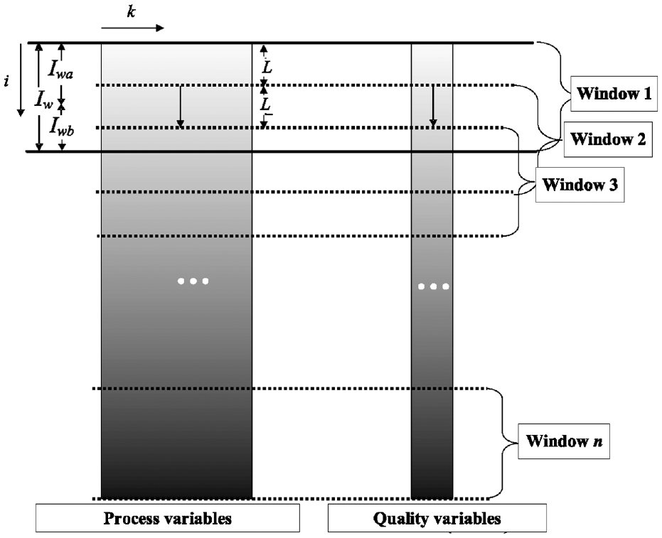
Schematic diagram of sliding window.
For multi-stage processes, due to the different effects of each stage on the final product quality, process variables in some stages will only have an impact on the final product quality after a longer period, so it is necessary to move these stages to make their variables correspond to the product quality after a later period, to obtain a more accurate correlation between process variables and quality variables. As shown in Figure 2, the overall data structure is adjusted, where the batch data of the second stage is moved back l batch to correspond to the quality variable data collected in the last batch. Thus, new process variable data and new quality variable data are obtained for modeling.
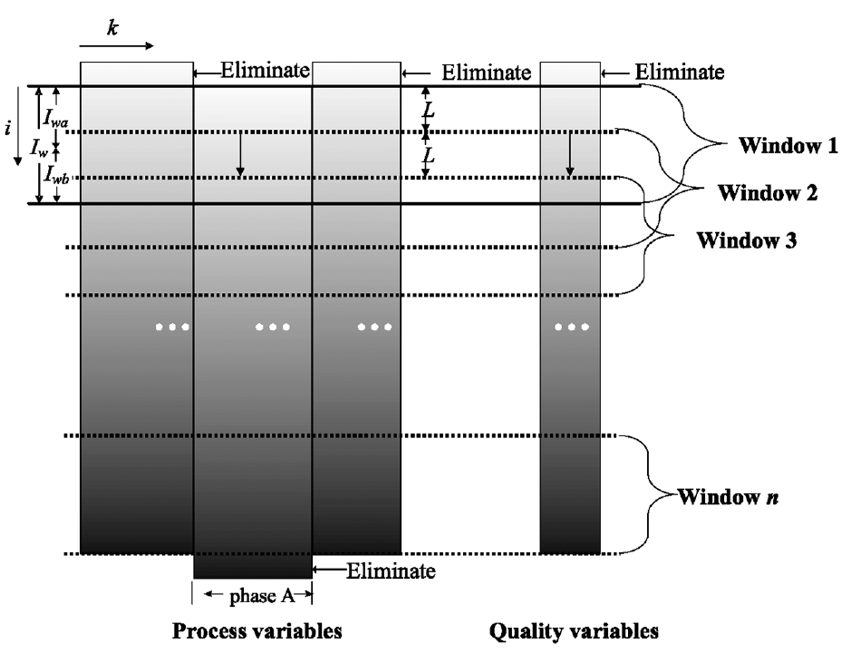
Improved data structure for stage movement.
Model migration based on JY-PLS
In actual production activities, moving the production of a class of products from one production site to another, or expanding a product from a pilot plant to an existing production plant, can be an expensive and difficult problem. In the construction of new batch process model, modeling problem is often caused by the insufficient running time of new process and the small amount of data collected by batch process. However, if the old process data is like the new process data, the model migration based on the similarity of the old data matrix can be realized, and the old data set can compensate the new process modeling data, to solve the problem of missing batch data of the new process. JY-PLS offers a solution based on the existing historical database for product transfer, which selects all variables of the old and new processes to extract data features, thus establishing regression models of hidden variables and obtaining public space information for model migration.
Suppose there are similar processes A and B, where A is the old process with more data and B is the new process with less data. The input matrix of process variables for process A and process B is
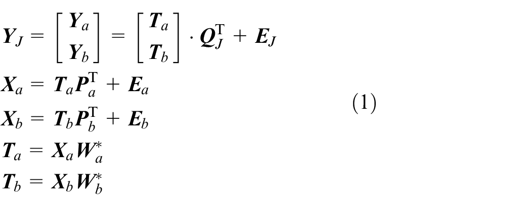
where
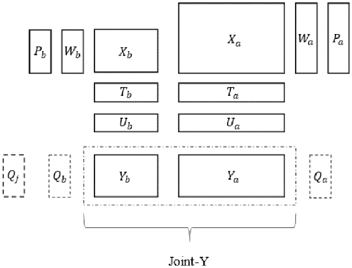
JY-PLS model.
When applying JY-PLS algorithm, the number of data columns in
Based on the stage moving sliding window modeling introduced above, the data in each window are divided into time slices to obtain the time slice model of JY-PLS:
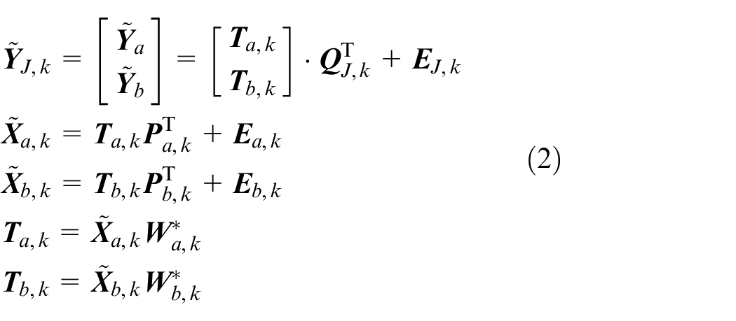
Among them,
After establishing the time slice model, the process variable
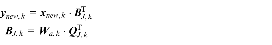
In this way, the establishment of JY-PLS prediction model has been completed.
Monitoring based on JY-PLS model migration method
After the JY-PLS model is obtained, the statistics and control limits required in the monitoring process can be calculated. In this paper, Hotell-T2 statistic in the principal subspace and SPE statistics in the residual space are selected as monitoring indicators. By monitoring the T2 statistic, the status of multiple principal elements can be synchronously monitored, to discover the fault of the running status in the batch process in time. As for SPE statistics, by measuring the projection of the sample vector in the residual subspace, the distance between the measured value and the offset of the principal component space is obtained. The calculation of SPE statistics includes the calculation of SPEx and SPEy.
Firstly, T2, SPEx and SPEy are calculated.
The T2 statistic is calculated as follows:
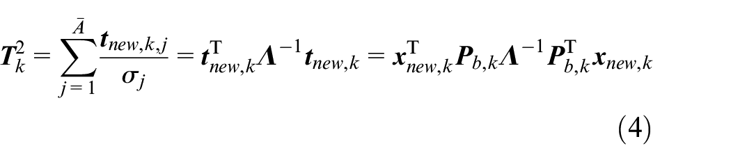
where
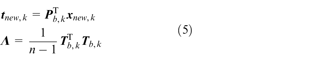
where
The formulae for calculating SPEx and SPEy statistics are as follows:
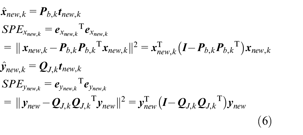
where
After completing the calculation of the statistics, the control limit of the corresponding statistics should also be calculated.
The control limit of T2 is calculated as follows:
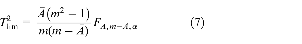
where m is the number of process variables in process B,
The control limit of SPEx is calculated as follows:
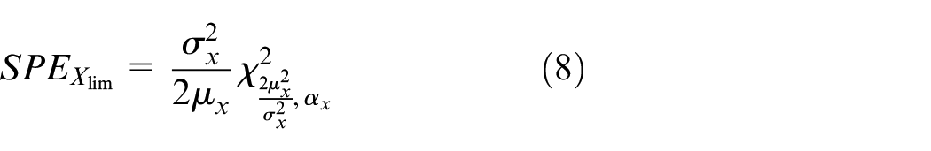
where
The control limit of SPEy is calculated as follows:
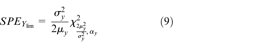
where
Illustration and discussions
Quality prediction using JY-PLS
In this paper, root mean square error (RMSE) is selected as the evaluation criterion for the prediction effect of the model.
The RMSE value is calculated as follows:

where
Based on the JY-PLS predictive modeling method introduced above, first the sliding window is established for the collected data, and the number of batches of each window is taken as 30, in which the first 20 batches are from process A and the last 10 batches are from process B. The sliding distance is 1, that is, each window moves 1 batch.
After the window is set up, the time slice models are established in each window. In each window, 919 time slices are obtained according to the sampling time, and the JY-PLS algorithm is used to build time slice models. It should be noticed that the number of time slices obtained for each window is the same.
For the JY-PLS model under each time slice, the next batch of the current window is taken as the test data, and is also divided into 919 time samples.
After following the above steps, quality prediction data of 31st–100th batches can be obtained, each of which has its own individual prediction under 919 time slices. The average of prediction data of all time slices in each batch is obtained and compared with that calculated by the traditional PLS modeling method using the sliding window. The prediction comparison is shown in Figure 4 as follows:
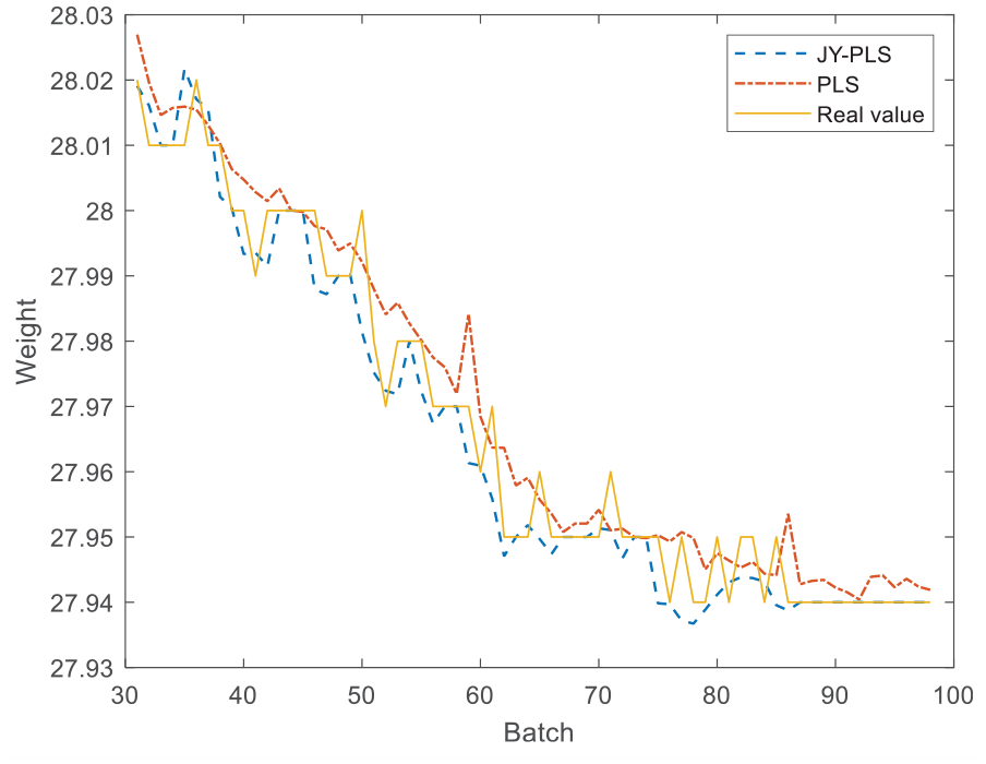
Prediction comparison between JY-PLS algorithm and traditional PLS algorithm.
At the same time, the root-mean-square error (RMSE) values of the two methods are calculated and listed in Table 1:
RMSE comparison between JY-PLS algorithm and traditional PLS algorithm.
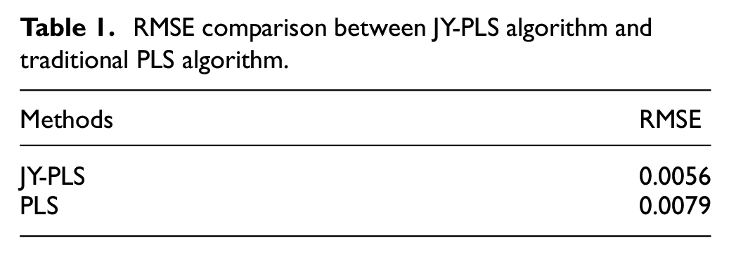
It can be seen from Figure 4 and Table 1 that the prediction effect of the JY-PLS algorithm is better than that of the traditional PLS algorithm, indicating that the transfer of old process data can well assist the establishment of the new model, and has better prediction performance than the traditional method.
Monitoring using JY-PLS
In this part, the JY-PLS model is established in each sliding window, and the relevant statistics and control limits are calculated to complete the simulation and monitoring of the injection molding start-up process.
All batches in each window are selected as training data, and three batches after each window are selected as test data. To show the monitoring result, window 5, window 12, window 24 and window 30 are selected as examples, and the monitoring results are compared with those obtained by the traditional sliding window using the PLS algorithm for online monitoring. Since the start-up process has more dynamic characteristic during the first half, which needs more attention, the windows are selected from the first half for monitoring to show the results. The monitoring results and comparison are shown as follows.
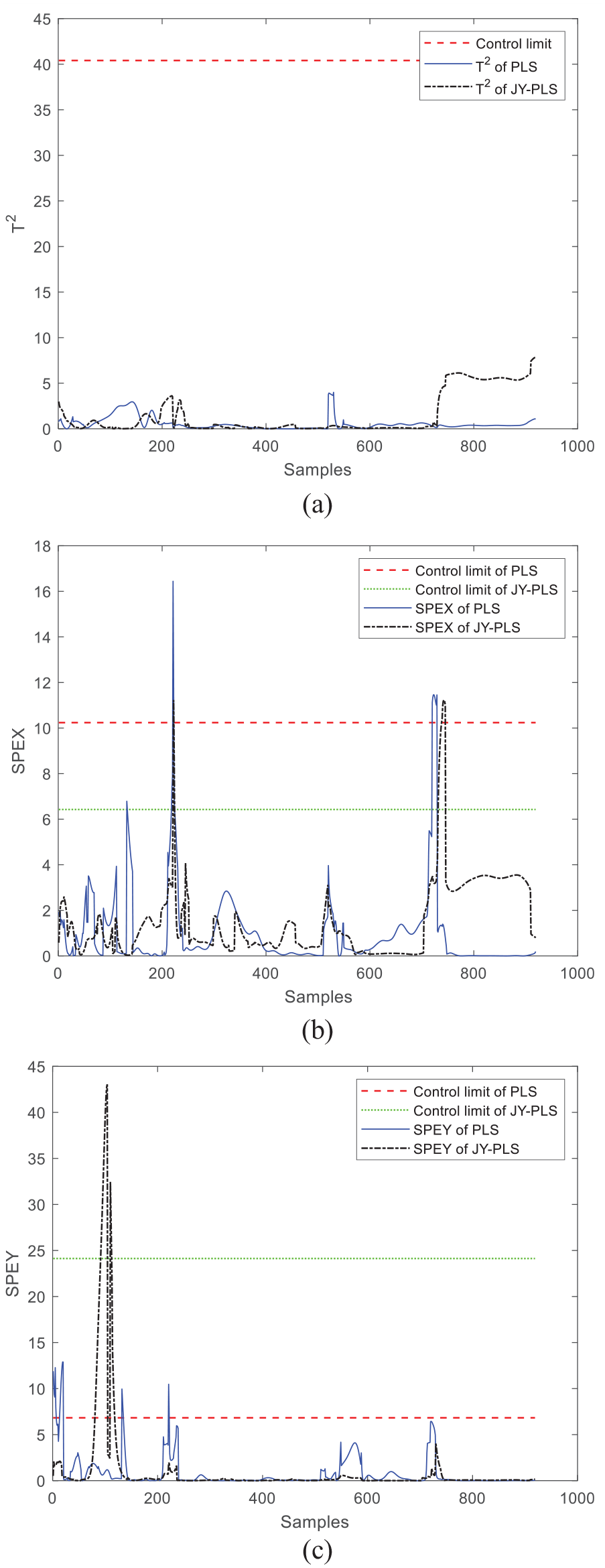
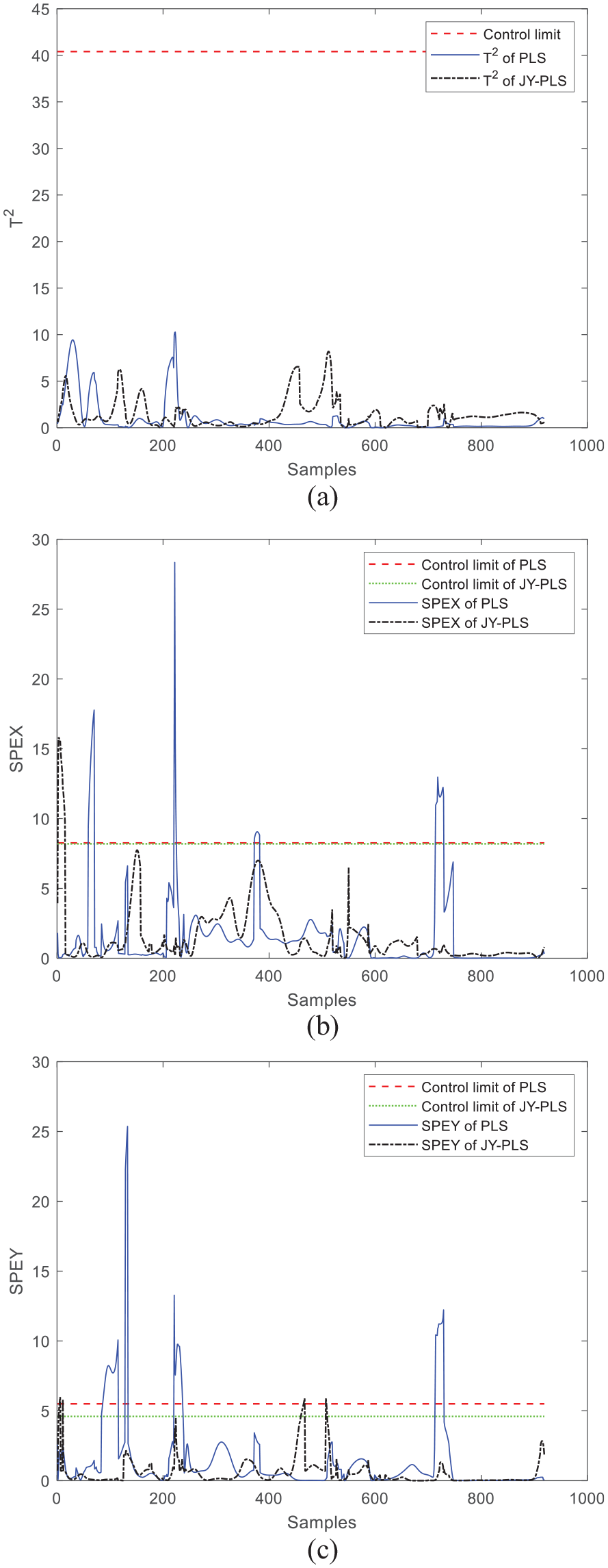
As can be seen from the comparison between Figures 5 and 6, the monitoring effect of window 5 and window 12 modeled by JY-PLS is good, and T2, SPEx, and SPEy, are not out of the control limits, indicating that the operation process is stable and no fault occurs. In the monitoring graph of window 5 using the PLS modeling method, the T2 statistic is stable below the control limit, but SPEx and SPEy occasionally exceed the control limit, indicating that the monitoring effect of the PLS algorithm is less stable than that of the JY-PLS algorithm.
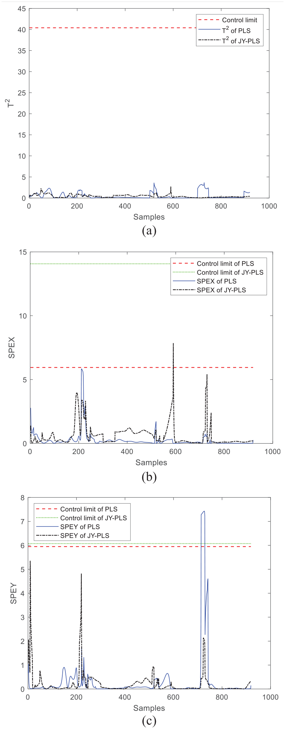
Comparison of online monitoring effects between JY-PLS algorithm and traditional PLS algorithm within window 5: (a) T2, (b) SPEx, and (c) SPEy.
Comparison of online monitoring effects between JY-PLS algorithm and traditional PLS algorithm within window 12: (a) T2, (b) SPEx, and (c) SPEy.
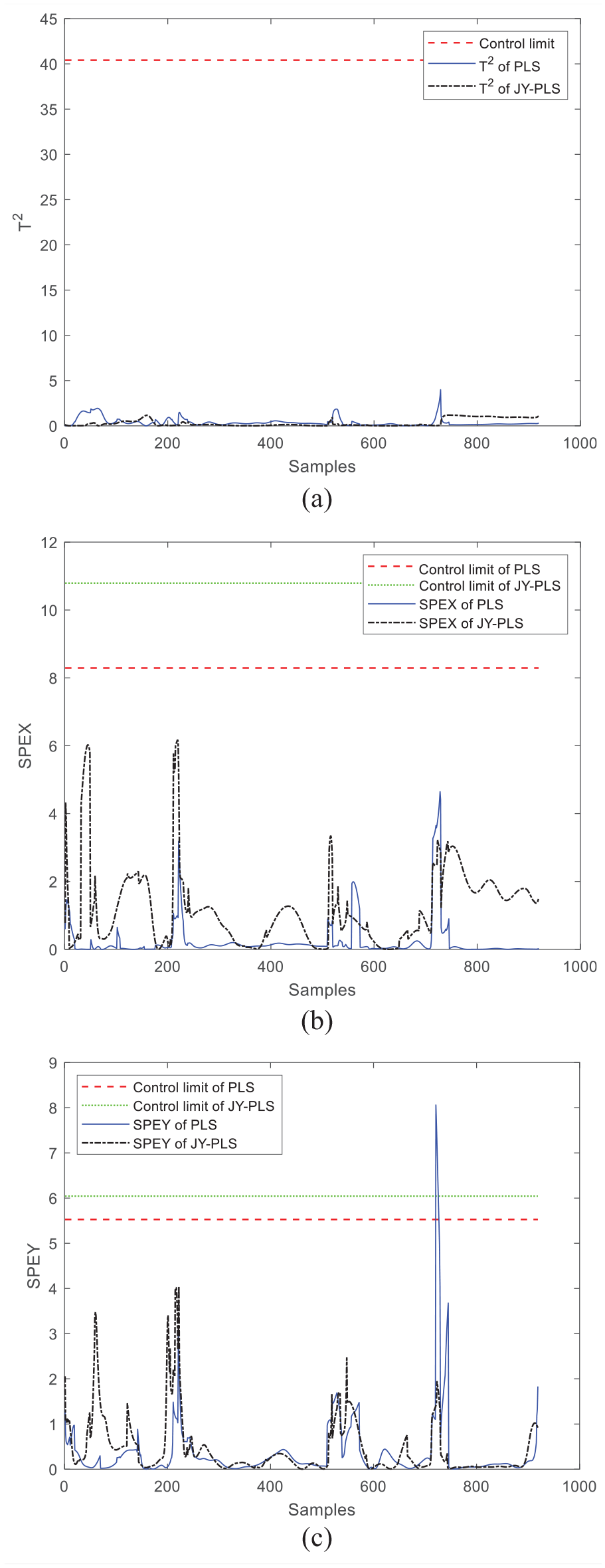
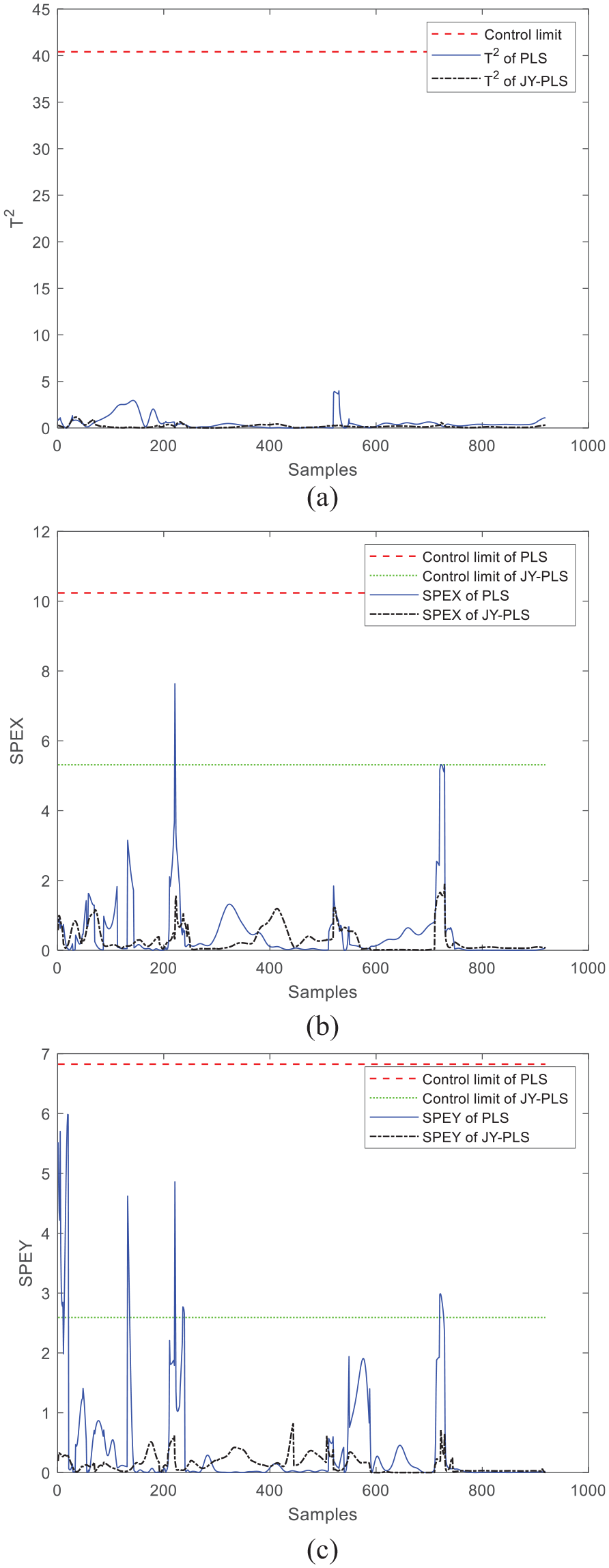
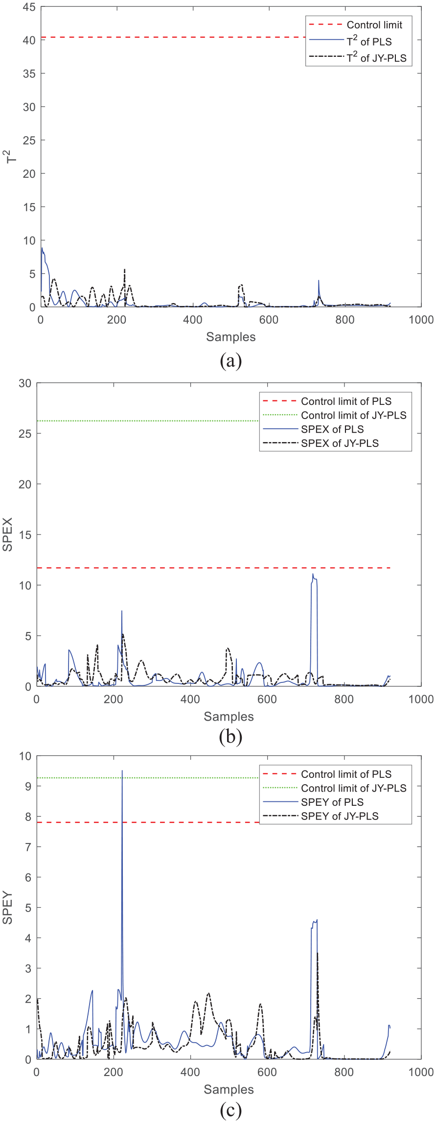
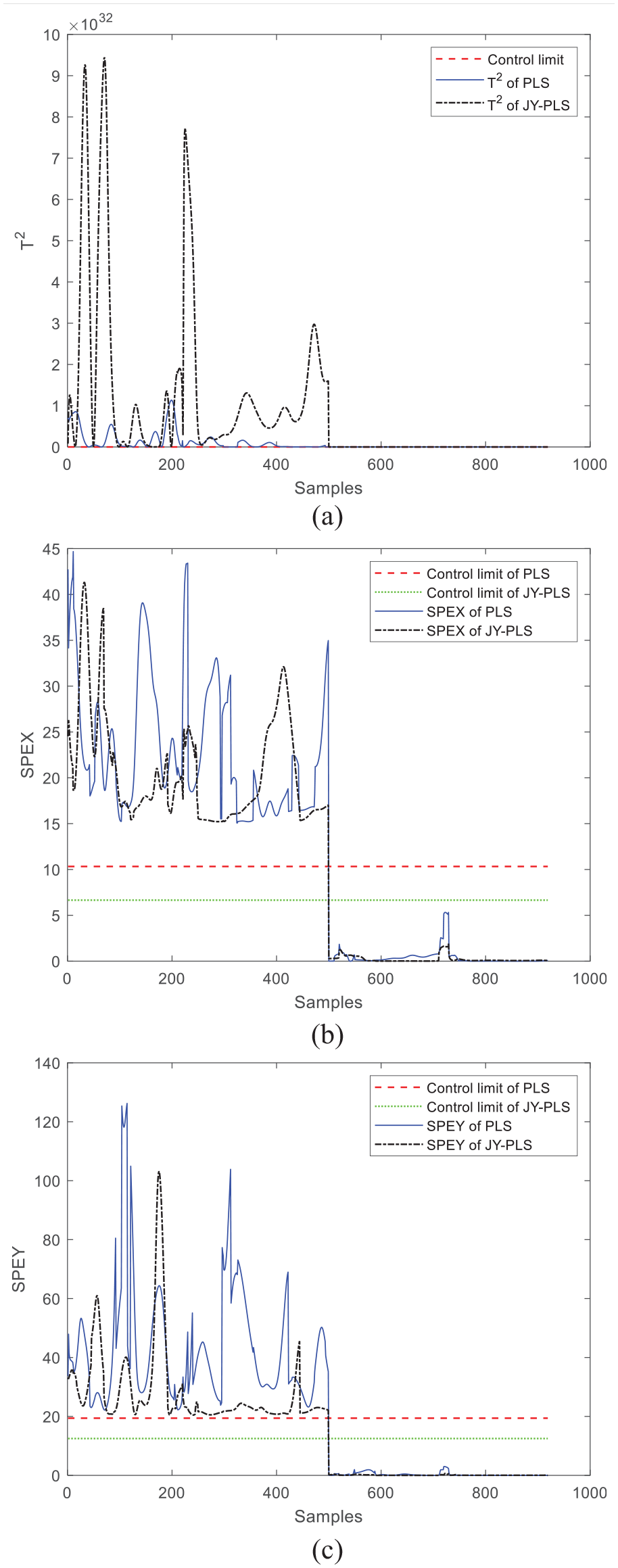
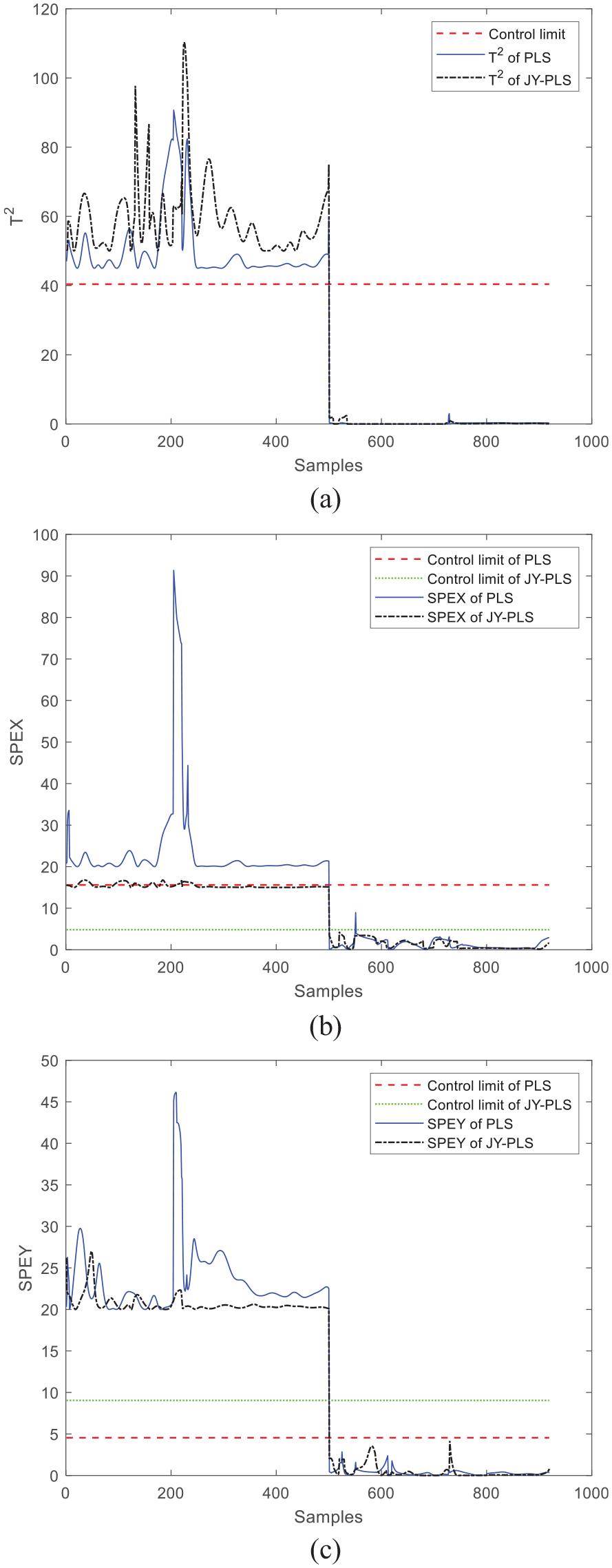
Next, the monitoring results of window 24 and window 30 are discussed. As can be seen from the comparison between Figures 7 and 8, T2 statistics of the JY-PLS algorithm model and the PLS algorithm model do not exceed the control limit when monitoring window 24 and window 30, but both of SPEx and SPEy have exceeded the limit, which proves that certain faults occur during operation and the monitoring effect is not ideal. Therefore, it is necessary to improve the monitoring model, put forward a new modeling method that moves the plasticizing stage back, and verify its effectiveness through online monitoring.
Comparison of online monitoring effects between JY-PLS algorithm and traditional PLS algorithm within window 24: (a) T2, (b) SPEx, and (c) SPEy.
Comparison of online monitoring effects between JY-PLS algorithm and traditional PLS algorithm within window 30: (a) T2, (b) SPEx, and (c) SPEy.
Monitoring based on stage moving JY-PLS model migration method
After completing the preliminary monitoring, considering the special impact of the plasticization stage on the reaction process mentioned earlier, further improvements were made to the online monitoring model: the entire batch of plasticization stage was moved back by one batch, and monitoring simulation was carried out after model correction, and compared with the original monitoring method to verify the effectiveness of the backward movement of plasticization stage in improving the monitoring model.
The injection molding process can be divided into four parts according to time periods: injection stage, pressure holding stage, plasticization stage, and cooling stage. During this process, during the plasticization stage, due to the fact that the plastic melt inside the screw cannot be fully applied during injection, it has not been fully injected into the mold cavity of this batch, and there is still a large amount of raw material present in the screw until the next batch arrives before injection is pushed forward. Therefore, it can be inferred that the plasticization stage will have a greater impact on subsequent batches. So, adjustments can be made to the overall data structure by moving the batch data within the time slot of the plasticization stage back one batch as a whole, corresponding to the quality variable data collected from the next batch. The quality variable data from the first batch and the process variable data from the 100th batch of plasticization stage can be discarded to obtain new process variable data and new quality variable data.
After improving the sliding window model with the method of stage moving, the new model is used for monitoring.
In the monitoring modeling of each window, all the data in each window is selected as the training data, and three batches after each window are selected as the test data. The monitoring simulation is conducted again for window 24 and window 30 with poor monitoring effect in the previous section, and the monitoring effect of the proposed new model is as follows.
As can be seen from the comparison between Figures 9 and 10, compared with the traditional monitoring methods, the monitoring model based on the plastination stage moving JY-PLS algorithm has a more stable performance in T2 statistics.
Online monitoring effects using stage moving JY-PLS algorithm and stage moving PLS algorithm within window 24: (a) T2, (b) SPEx, and (c) SPEy.
Online monitoring effects using stage moving JY-PLS algorithm and stage moving PLS algorithm within window 30: (a) T2, (b) SPEx, and (c) SPEy.
Compared with window 24 and window 30, the SPEx and SPEy statistics of the improved method are both stable within the control limit, except that the SPEy statistics of window 30 after the improved modeling by the PLS algorithm are slightly over limit, indicating that the improved monitoring effect of the JY-PLS model is better than that of the PLS model.
Figures 11 and 12 show the comparison of the monitoring effect between the traditional method and the improved method using the JY-PLS algorithm. It can be seen that the original over-limit SPEx and SPEy have been improved after the improvement, and it is confirmed that the monitoring effect of the proposed plastination stage moving JY-PLS algorithm is better than that of the traditional model.
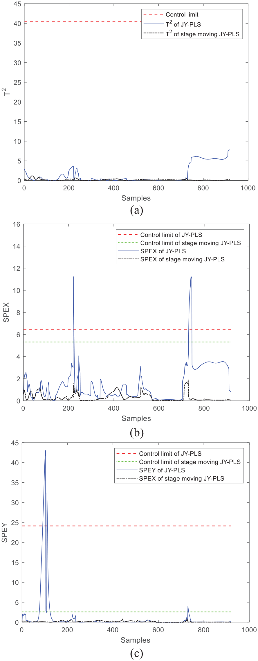
Comparison of online monitoring effects between stage moving JY-PLS algorithm and JY-PLS algorithm within window 24: (a) T2, (b) SPEx, and (c) SPEy.
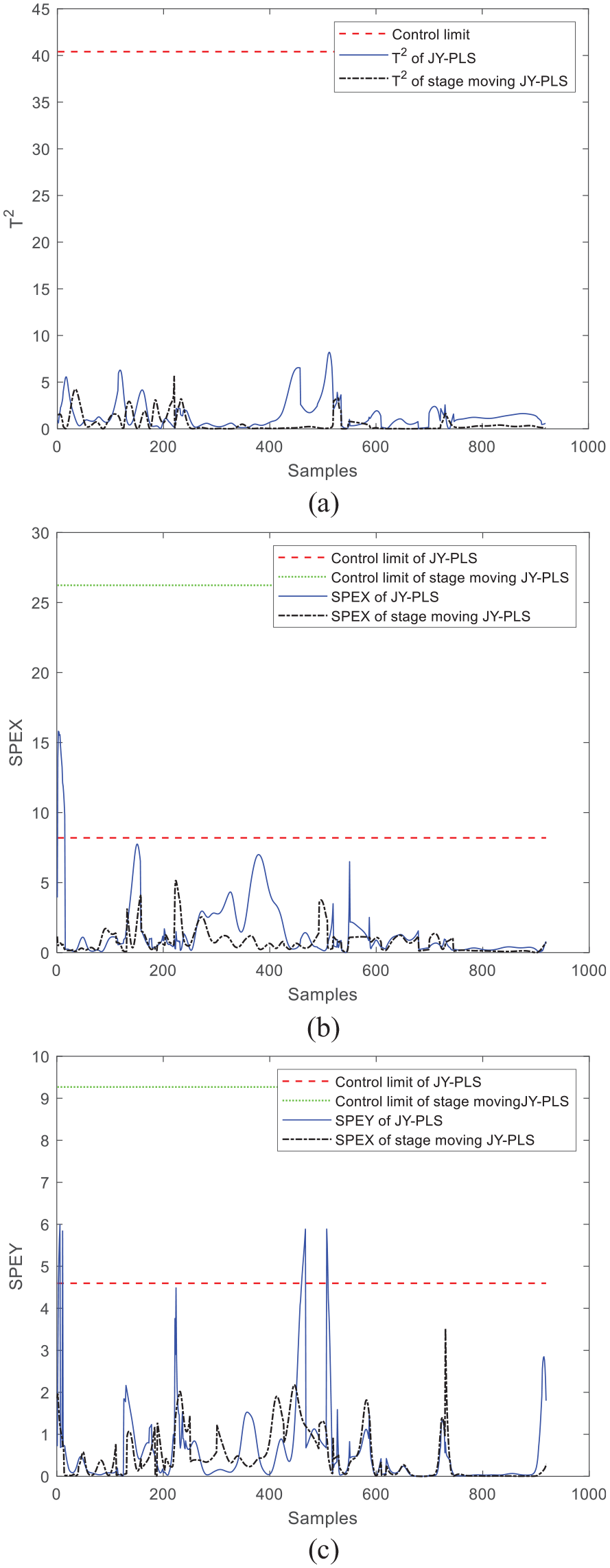
Comparison of online monitoring effects between stage moving JY-PLS algorithm and JY-PLS algorithm within window 30: (a) T2, (b) SPEx, and (c) SPEy.
Fault monitoring
In order to further verify the effectiveness of the monitoring effect of the proposed stage moving JY-PLS model, fault simulation is carried out on the data in the monitoring process. Specific verification methods are as follows:
The fault simulation in this section includes the simulation of the JY-PLS algorithm and the PLS algorithm when two kinds of faults occur: the fault when a variable is constant 0 (i.e. the variable data cannot be detected), and the fault when a variable is constant.
(1) When a variable cannot be detected normally, the fault simulation monitoring results are mainly set as follows:
Window 24 is selected, which has good monitoring effect in the previous section, as the experimental window, and it is ensured that the training batch remains unchanged to establish a normal monitoring model; For the test batch data, the measured value of the cylinder pressure when k = 1∼500 is changed to 0, and all process variable data remained unchanged when k = 501–919, so as to simulate the monitoring effect when the data of the time slice variable of 1–500 could not be detected normally, as shown in Figure 13.
(2) The simulation monitoring results when a variable fails and maintains a constant value are mainly set as follows:
Fault monitoring effect when variables cannot be monitored normally: (a) T2, (b) SPEx, and (c) SPEy.
Window 24 is selected, which has good monitoring effect in the previous section, as the experimental window, and it is ensured that the training batch remains unchanged to establish a normal monitoring model; For the test batch data, the measured value of the cylinder pressure when k = 1–500 is changed to 99, and all process variable data remain unchanged when k = 501–919, so as to simulate the monitoring effect when the data of the 1–500 time slice variable failed and the constant value remains unchanged, as shown in Figure 14.
Fault monitoring effect when variables remain constant: (a) T2, (b) SPEx, and (c) SPEy.
It can be seen from the simulation results of fault simulation that for the JY-PLS and PLS algorithms, when variables cannot be measured normally and variables remain constant due to faults, T2, SPEx, and SPEy statistics all have obvious overlimit conditions, indicating that process anomalies can be accurately monitored. When the test data returned to normal, the statistics under the corresponding time slice also returned to below the control limit, indicating that the monitoring process returned to normal. The correctness and effectiveness of the improved monitoring model are also verified by the fault simulation.
Conclusions
This article first improves the sliding window method by proposing a stage moving sliding window. At the same time, a prediction model based on the JY-PLS algorithm is proposed, and the statistics and corresponding control limits of online monitoring based on the JY-PLS model with stage moving are calculated. In the application of batch process start-up process, the prediction simulation of the JY-PLS model is completed, and the effectiveness of model migration under JY-PLS algorithm has been verified by comparing the RMSE value of the prediction results with the traditional PLS algorithm. The effectiveness of online monitoring method based on the JY-PLS model has also been verified. Furthermore, since the impact of the plasticization stage on subsequent batches is greater than that of the current batch in the injection molding process, the proposed stage moving sliding window is applied to slice the plasticization stage time backwards. Based on this, the JY-PLS model is established and process monitoring is completed. Compared with the traditional methods, it has improved the situation of exceeding limits in process monitoring and significantly improved the monitoring effect. In addition, simulation monitoring is carried out on the situation when variables failed, and the simulation results of fault simulation also to some extent confirm the effectiveness of process monitoring using the stage moving JY-PLS model.
Footnotes
Acknowledgements
This work is supported in part by National Natural Science Foundation of China (No. 61503069) and the Fundamental Research Funds for the Central Universities (N2404010).
Declaration of conflicting interests
The author(s) declared no potential conflicts of interest with respect to the research, authorship, and/or publication of this article.
Funding
The author(s) disclosed receipt of the following financial support for the research, authorship, and/or publication of this article: This work is supported in part by National Natural Science Foundation of China (No. 61503069) and the Fundamental Research Funds for the Central Universities (N2404010).