Sage Journals: Discover world-class research

Abstract

The manuscript introduces a novel approach to design and construct a pore water pressure sensor utilizing strain gage technology integrated with deep learning principles. This sensor type is specifically tailored for measuring pressure at the vertex of pile bases in structures with substantial load-bearing capacity. While existing pressure sensors employing strain gage technology are available, this research addresses a unique measurement model suited for deep-water environments characterized by high corrosiveness and heavy loads. Consequently, the manuscript proposes design innovations aimed at optimizing the sensor’s form and dimensions to accommodate these demanding conditions. Computational simulations are conducted to perform relevant calculations, with results validated through rigorous analysis and experimentation against real-world datasets. Moreover, the study incorporates a pioneering deep learning-based data acquisition model to enhance output values, a feature currently underutilized in sensor technology. The findings demonstrate the viability of the proposed water pressure sensor model in various challenging working environments. This research underscores the potential for proactive manufacturing of sensors in diverse configurations, emphasizing adaptability and efficiency.

Keywords

Sensor pressure water in pores deep learning pile foundation constructions

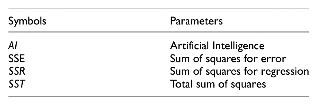
Symbols and parameters used in the analysis

Symbols	Parameters
AI	Artificial Intelligence
SSE	Sum of squares for error
SSR	Sum of squares for regression
SST	Total sum of squares

Introduction

Sensors have become increasingly important in our lives, thanks to the rapid development of science and technology.^1,2 They serve as intermediaries between objects that perform tasks and objects that make decisions. In this context, the construction industry has made significant progress in both quantity and quality by utilizing sensors.³ The use of sensors in construction^4,5 has increased economic efficiency and improved safety monitoring for buildings. Pressure sensors are widely applied in construction engineering, particularly in pile foundation systems. They can accurately determine pressure values for fluids,^6–9 solids,^8,10–12 and force impacts,^13–16 enabling precise control of the working process and ensuring the overall safety of the construction system. The pressure sensor’s operating principle is based on the change in deformation signal before and after being impacted by external conditions. Various principles are used for this purpose, such as the piezoresistive principle,^17–20 inductive principle,^21–24 capacitive principle,^25–28 piezoelectric principle,^29–33 thermo-electric principle,^34–37 and acoustic principle.^38–40 New technologies have brought many positive changes to measuring the properties of various mechanical systems. However, for mechanical systems with complex impact conditions, high intensity, and large corrosive environments, such as pile foundation systems, these technologies are often inadequate. Therefore, strain gage technology^41–44 has been proposed as a suitable choice for creating soil pressure sensors for mechanical systems, like pile foundations. Strain gage technology measures deformation in fluid mechanical elements (such as water and gas)^45–47 and discrete mechanics (such as soil and sand)^48–51 based on their mechanical properties. When a force is exerted on the measuring diaphragm, it changes the original characteristics and creates deformation on the measuring diaphragm. The elements used can take the form of cylinders,⁵² tube springs,^53,54 siphons,^55,56 or elastic diaphragms,^57,58 and must have good resilience to meet the requirements of complex working conditions.^59,60 The pressure sensor is manufactured using a strain gage sensor fixed on an elastic diaphragm (thin diaphragm). The connection forms a Wheatstone bridge circuit to create a measuring system. In the absence of pressure acting on the diaphragm, the bridge circuit is in equilibrium, and the output voltage is zero. When the device is inserted into a working environment, such as buried underground, underwater, or a mixed environment, the elastic diaphragm will deform due to pressure from the environment. This leads to a change in the resistance value in the bridge circuit. Specifically, if the resistance near the center of the diaphragm decreases, the resistance at the peripheral circumference will increase, and vice versa. As a result, the bridge circuit becomes unbalanced, and the output voltage is non-zero. The change in resistance value depends on the magnitude of the diaphragm’s deformation caused by the external load. Therefore, the output voltage signal reflects the imbalance of the bridge circuit in various pressure impacting scenarios. The corresponding pressure magnitude acting on the diaphragm can be calculated by measuring the output voltage. Thus, the strain gage pressure sensor essentially measures the deformation of the elastic diaphragm.

Artificial Intelligence (AI) models have widely penetrated modern sensor systems, transforming their functionalities and capabilities. AI-integrated sensor systems^61,62 offer significantly improved sensing solutions in terms of accuracy, efficiency, and flexibility. In environmental monitoring, AI-driven sensor systems^63,64 utilize complex algorithms to accurately detect and measure pollutants, gases, and other environmental factors, enabling more effective pollution control measures and early warning systems for natural disasters. Moreover, AI-guided sensor networks are reshaping smart infrastructure and urban planning, promoting intelligent traffic management,^65,66 optimizing energy consumption, and predictive maintenance of critical infrastructure, enhancing overall sustainability and resilience of cities. In industrial environments, AI-enabled sensors facilitate predictive maintenance^64,67 quality control, and process optimization, leading to increased productivity and reduced downtime by leveraging machine learning algorithms to identify potential equipment failures in advance, minimizing disruptions and maximizing efficiency. In conclusion, integrating AI models into sensor systems signifies a significant transformation in data collection, analysis, and utilization, driving innovation across various fields and paving the way for a more connected and intelligent world.

The following manuscript details a comprehensive investigation into the design, production, and utilization of a soil pressure measurement sensor system tailored for pile foundation systems within the construction industry, specifically engineered to perform effectively in intricate operational environments. The research unfolds in two distinct phases: (1) a laboratory-oriented assessment of soil pressure measurements to ascertain the outcomes and (2) the real-world application of the sensor system to an actual pile foundation setup, where pre-existing conditions might impact the functionality of the sensor system. In order to accommodate the demands posed by these intricate working conditions, the study has thoughtfully selected materials that offer ease of processing, exhibit consistent mechanical properties, and ensure optimal elasticity during the tension-compression procedures required for the construction of elastic diaphragms. Furthermore, a signal acquisition model grounded in deep learning methodologies has been adopted to enhance the efficiency of data acquisition from the sensor system. This constitutes a significant advancement over the current data acquisition system employed for the sensor, enabling its operation across diverse scenarios and significantly improving the precision of the data obtained.

Theoretical basis

Deformation properties of elastic diaphragm

Strain gages are fixed on an elastic diaphragm,^57,58 which is usually composed of a thin sheet of metal. The strain gages are connected to form a Wheatstone bridge circuit.^68–70 The elastic diaphragm used in this research is a flat, thin, round metal sheet with good compression-tension capacity, which is used to demonstrate the relationship between the pressure of the impacting force and the deformation. Let P be the pressure exerted by the soil on the diaphragm. At the initial moment, the pressure P is zero, so the diaphragm deformation is also zero, as shown in Figure 1.

Figure 1.

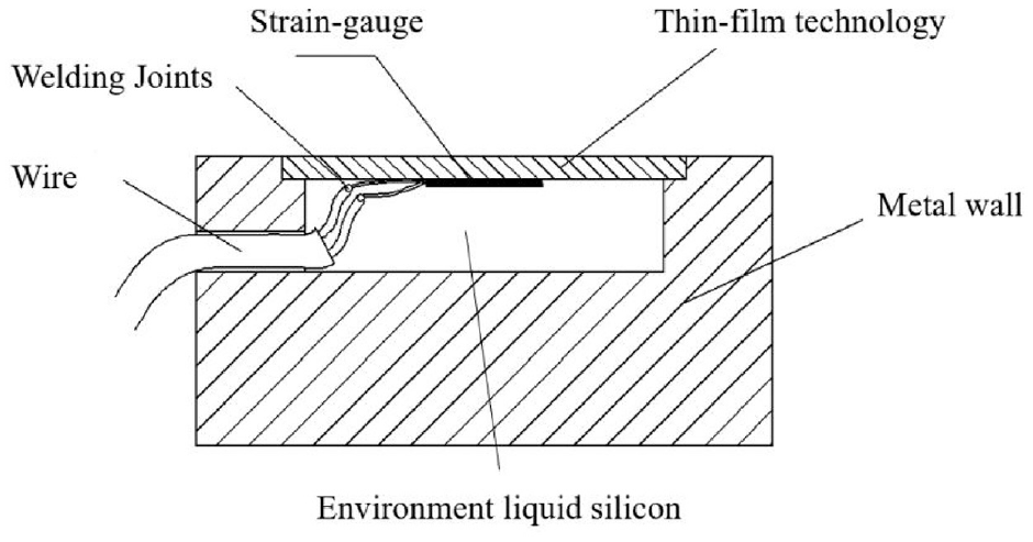
Overall model of the sensor of water pressure measurement.

In the case of fluid compression increasing the pressure value on the sensor, the elastic diaphragm will be deformed. The displacement value at the center of the elastic diaphragm is determined by equation (1):

y = \frac{3 . P . R_{0}^{4} . (1 - ν^{2})}{16 . t^{3} . E}

(1)

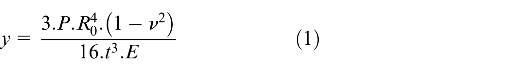
in which y represents the translocation at the center of the elastic diaphragm, P is the static pressure impacting on the diaphragm, R_o is the radius of the diaphragm, ν is the Poisson’s ratio of the material used for fabrication, t is the thickness of the diaphragm, and E is the elastic modulus of the material. The translocation of the diaphragm increases with the increase in pressure applied, resulting in an increase in deformation of the diaphragm. The deformation of the elastic diaphragm is divided into two components, the tangential direction (ϵT) and the radial direction (ϵR), as shown in Figure 2.

Figure 2.

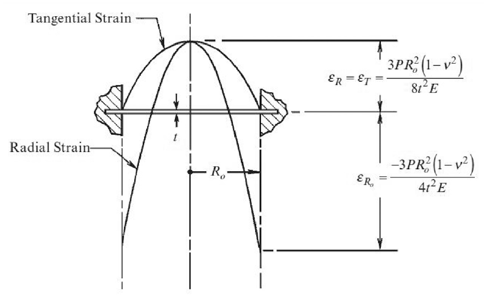
Graph demonstrates the deformation of the elastic diaphragm.

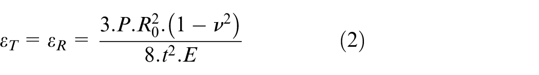
We can see from the graph that demonstrates the deformation of the elastic diaphragm in the tangential direction and centripetal direction at the center of the elastic diaphragm, which are calculated using equation (2) due to symmetry:

ε_{T} = ε_{R} = \frac{3 . P . R_{0}^{2} . (1 - ν^{2})}{8 . t^{2} . E}

(2)

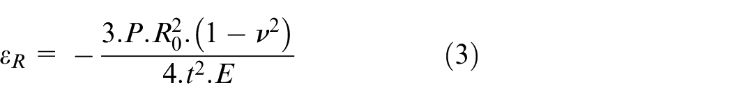
In the increasing direction of the elastic diaphragm radius to the maximum value, the value ϵT gradually decreases to zero, and ϵR approaches the minimum value as shown in equation (3).

ε_{R} = - \frac{3 . P . R_{0}^{2} . (1 - ν^{2})}{4 . t^{2} . E}

(3)

Wheatstone bridge circuit model

We have established a Wheatstone bridge circuit that is balanced based on small changes in the component resistance of the strain gage. This is a common method for manufacturing pressure sensors used to measure the diaphragm’s deformation value. A well-functioning sensor can read very small deformation values with high accuracy. The basic Wheatstone bridge circuit consists of four resistors, R₁, R₂, R₃, and R₄. The excitation voltage, usually 10 V, is denoted as VS, while V₀ represents the measured voltage. The electrical circuit can be formed through the connections, as shown in Figure 3.

Figure 3.

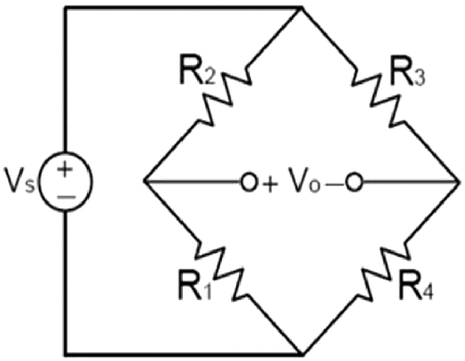
Wheatstone bridge circuit.

Depending on the specific purpose and object to be measured, we can use 1, 2, or 4 strain gage configurations when designing a Wheatstone balanced bridge circuit to measure deformation on diaphragms or thin plates, assuming R₁ = R₂ = R₃ = R₄ = R.

- Configuration of 1 strain gage (quarter bridge)

In the Wheatstone bridge circuit shown in Figure 4, one of the four resistors R₁, R₂, R₃, or R₄ is replaced with a strain gage, while the other three resistors remain constant. This configuration is known as a quarter bridge circuit, and it is widely used for measuring deformation due to its simplicity.

Figure 4.

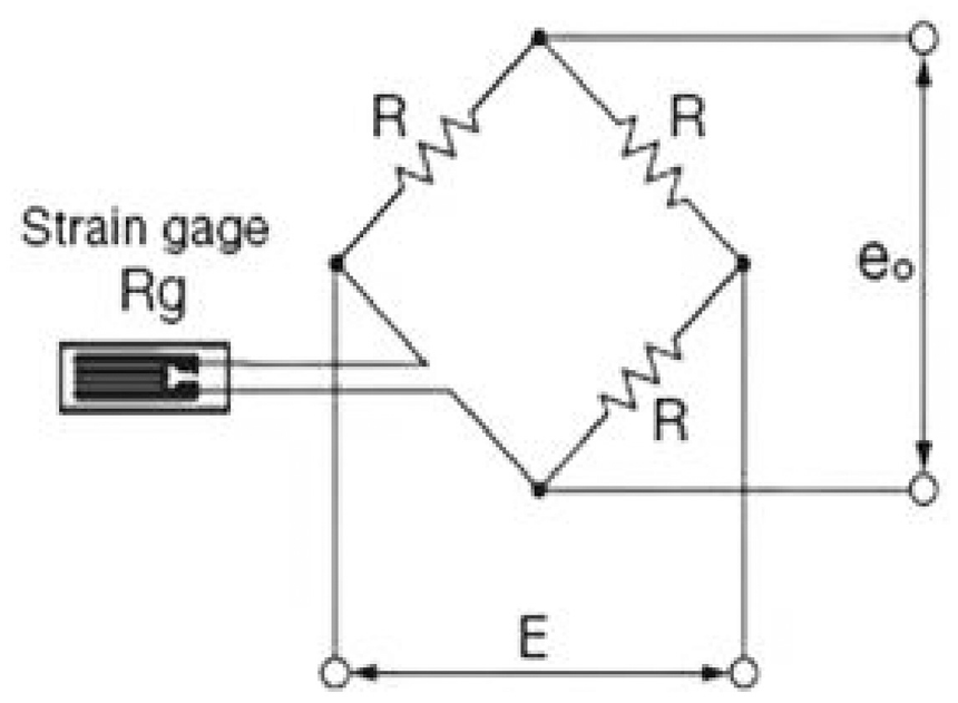
Quarter bridge circuit.

- Configuration of 2 strain gage (haft bridge)

In the circuit, two fixed resistors are replaced with two strain gages, while the other two resistors remain constant. The two strain gages can be positioned next to each other or opposite each other. When positioned next to each other, as shown in Figure 5(a), one strain gage operates while the other compensates for the balance point. When positioned opposite each other, as shown in Figure 5(b), both strain gages operate, and the circuit is self-compensating according to theory.

Figure 5.

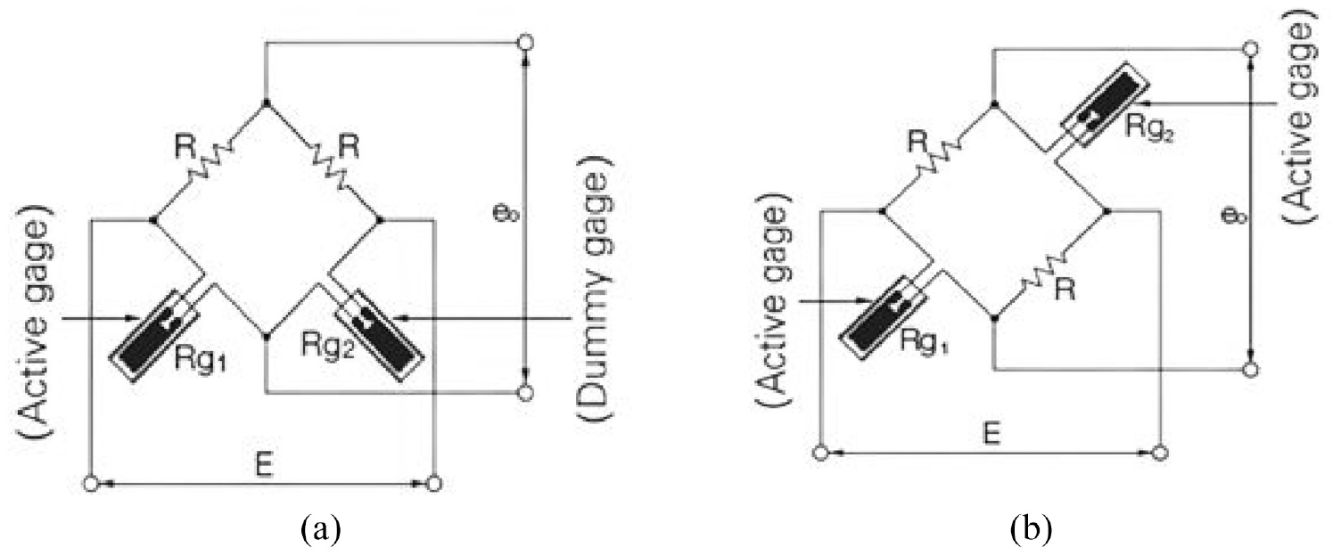
Haft bridge circuit: (a) two strain gages are next to each other and (b) two strain gages are opposite each other.

- Configuration of 4 strain gage (full bridge)

This configuration uses all four strain gages in a Wheatstone bridge circuit, with two gages mounted on the surface of the diaphragm under tension and the other two gages mounted on the surface of the diaphragm under compression. When the diaphragm deforms, the resistance of the strain gages changes, causing an unbalanced voltage in the Wheatstone bridge. The magnitude of the unbalanced voltage is proportional to the deformation, and can be measured and used to calculate the strain. In the full bridge circuit, four fixed resistors are replaced with four strain gages that are connected to the circuit. This configuration allows for a larger voltage signal and better compensation of the balance point, which helps eliminate the effects of external factors that may cause deformation. Figure 6 illustrates this configuration.

Figure 6.

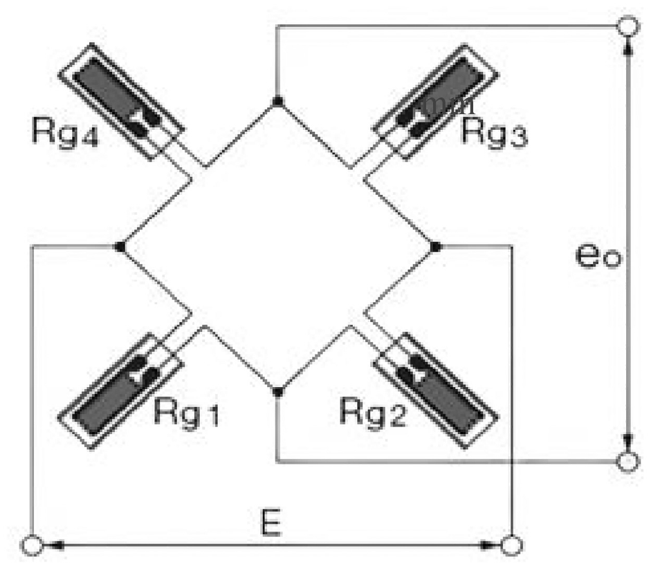
Full bridge circuit.

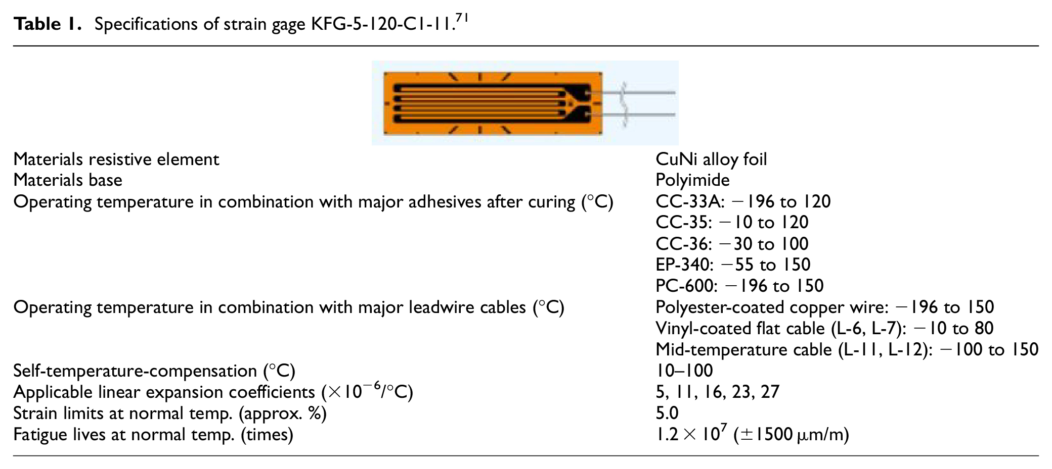
Table 1 provides a detailed specification of the strain gage used in this research.

Table 1.

Specifications of strain gage KFG-5-120-C1-11.⁷¹


Materials resistive element	CuNi alloy foil
Materials base	Polyimide
Operating temperature in combination with major adhesives after curing (°C)	CC-33A: −196 to 120
	CC-35: −10 to 120
	CC-36: −30 to 100
	EP-340: −55 to 150
	PC-600: −196 to 150
Operating temperature in combination with major leadwire cables (°C)	Polyester-coated copper wire: −196 to 150
	Vinyl-coated flat cable (L-6, L-7): −10 to 80
	Mid-temperature cable (L-11, L-12): −100 to 150
Self-temperature-compensation (°C)	10–100
Applicable linear expansion coefficients (×10⁻⁶/°C)	5, 11, 16, 23, 27
Strain limits at normal temp. (approx. %)	5.0
Fatigue lives at normal temp. (times)	1.2 × 10⁷ (±1500 μm/m)

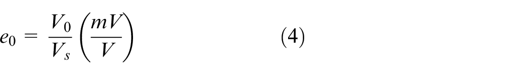
The excitation voltage is denoted as V_s (V), while V₀ (mV) represents the output voltage that needs to be measured. The voltage magnitude displayed by the unit is denoted as e₀, as shown in Abbasi et al.⁵

e_{0} = \frac{V_{0}}{V_{s}} (\frac{mV}{V})

(4)

Ratio $e_{0} = \frac{V_{0}}{V_{s}}$ is defined as follow:

e_{0} = \frac{V_{0}}{V_{s}} = \frac{R_{1}}{R_{1} + R_{2}} - \frac{R_{4}}{R_{3} + R_{4}} = \frac{R_{1} R_{3} - R_{2} R_{4}}{(R_{1} + R_{2}) (R_{3} + R_{4})}

(5)

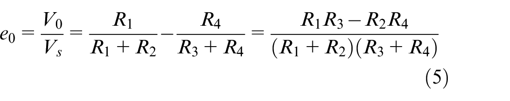
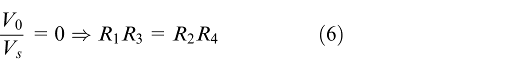
The condition for a balanced bridge circuit can be derived from the equation above. If there is no external pressure acting on the system, the measured output voltage should be equal to 0 (mV/V)

\frac{V_{0}}{V_{s}} = 0 \Rightarrow R_{1} R_{3} = R_{2} R_{4}

(6)

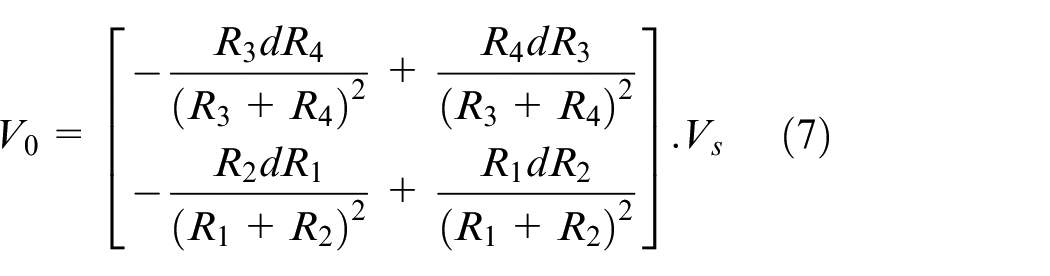
As the voltage increases, the deformation of the strain gage results in a change in resistance in the circuit. Consequently, the output voltage is non-zero and can be determined as follows:

V_{0} = [\begin{matrix} - \frac{R_{3} d R_{4}}{{(R_{3} + R_{4})}^{2}} + \frac{R_{4} d R_{3}}{{(R_{3} + R_{4})}^{2}} \\ - \frac{R_{2} d R_{1}}{{(R_{1} + R_{2})}^{2}} + \frac{R_{1} d R_{2}}{{(R_{1} + R_{2})}^{2}} \end{matrix}] . V_{s}

(7)

The output voltage can be calculated directly from the deformation of the strain gage resistor bridges in the pressure sensor, as shown in Abbasi et al.⁵ The voltage output e₀ is directly proportional to the total deformation of each component resistor bridge. Let F be the gage factor of the strain gage; then, we have:

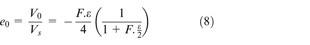
e_{0} = \frac{V_{0}}{V_{s}} = - \frac{F . ε}{4} (\frac{1}{1 + F . \frac{ε}{2}})

(8)

Substituting the above formula with F = 2.09 (gage factor coefficient of strain gage)

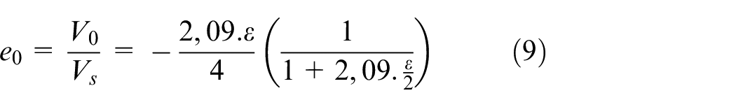
e_{0} = \frac{V_{0}}{V_{s}} = - \frac{2, 09 . ε}{4} (\frac{1}{1 + 2, 09 . \frac{ε}{2}})

(9)

For the full bridge circuit model, its disadvantage lies in the generation of heat during operation. To address this drawback, the research will rely on equation (9), which demonstrates that ϵ is the primary parameter influencing the model due to the thermal variations (temperature increase) of the strain gage negatively affecting measurement results. Therefore, the membrane model chosen for this study needs to be represented as a thin membrane with excellent heat dissipation capabilities, nearly instantaneous, to avoid influencing the measurement results. Furthermore, given the specific nature of the sensor model designed in this draft, it operates in a water, humid, or underground environment with significantly lower external temperatures compared to the actual environment. Consequently, this also provides an advantage in minimizing the temperature impact from the strain gage on the measurement results.

Mechanical theory in elastic diaphragms

An elastic diaphragm is a thin, round, flat plate with a thickness much smaller than its other dimensions. The plane that evenly divides the film thickness is referred to as the average plane or intermediate plane. The intersection line between the average face and lateral faces is called the tangent. The deformation level of the elastic diaphragm is demonstrated as the deformation of the average surface, which is also referred to as the elastic plane. In the case of thin plates, stress-strain in the direction perpendicular to the average face can be neglected. However, for the purposes of this research, several assumptions have been made regarding elastic diaphragms:

An element is straight and perpendicular to the average plane before deformation. After deformation, the element remains straight and perpendicular to the average plane. This illustrates that the elements in the face always operate in the elastic domain without any change during external impacting loads.

From the above assumption, we can infer that the layers parallel to the average surface will not slide over each other. This means that when the planes are parallel to the average face, they will not compress each other. This results in the elastic membrane always operating in a stable state without distortion and with the best output signals obtained.

The average surface only moves in the direction perpendicular to it. Thus, any translocation in the x and y directions is ignored.

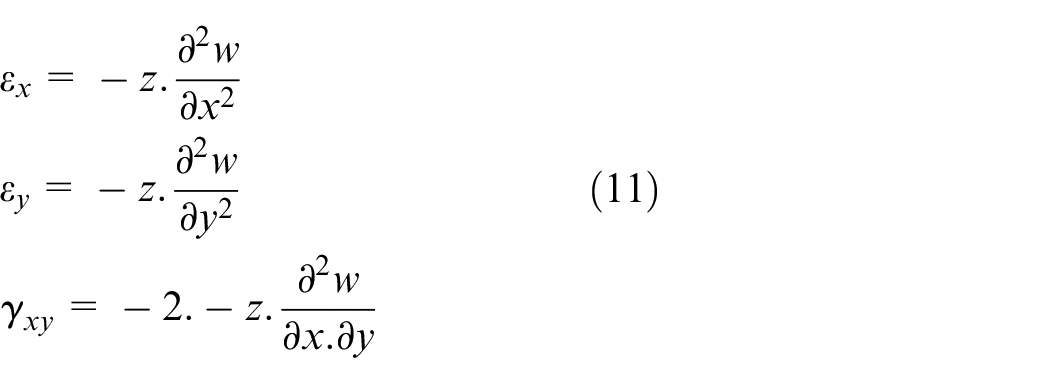
Based on the given assumptions, we can apply them to a thin circular plate with a constant thickness and uniformly distributed load in the direction perpendicular to the plate’s average plane. Let w be the displacement at a point on the average surface in the z-direction, the formulas for stress and strain on the plate surface are derived as follows [6]:

The stress on the diaphragm surface is illustrated in equation (10):

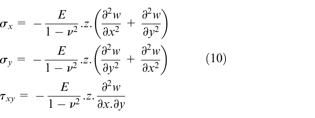
\begin{matrix} σ_{x} = - \frac{E}{1 - ν^{2}} . z . (\frac{\partial^{2} w}{\partial x^{2}} + \frac{\partial^{2} w}{\partial y^{2}}) \\ σ_{y} = - \frac{E}{1 - ν^{2}} . z . (\frac{\partial^{2} w}{\partial y^{2}} + \frac{\partial^{2} w}{\partial x^{2}}) \\ τ_{xy} = - \frac{E}{1 - ν^{2}} . z . \frac{\partial^{2} w}{\partial x . \partial y} \end{matrix}

(10)

The diaphragm deformation is calculated according to the translocation w(x,y)

\begin{matrix} ε_{x} = - z . \frac{\partial^{2} w}{\partial x^{2}} \\ ε_{y} = - z . \frac{\partial^{2} w}{\partial y^{2}} \\ γ_{xy} = - 2 . - z . \frac{\partial^{2} w}{\partial x . \partial y} \end{matrix}

(11)

According to the third assumption, as the deflection of average plane (w = w (x, y)) is independent of the z coordinate, the stresses are all linear functions of z. Their distribution is shown in Figure 7.

Figure 7.

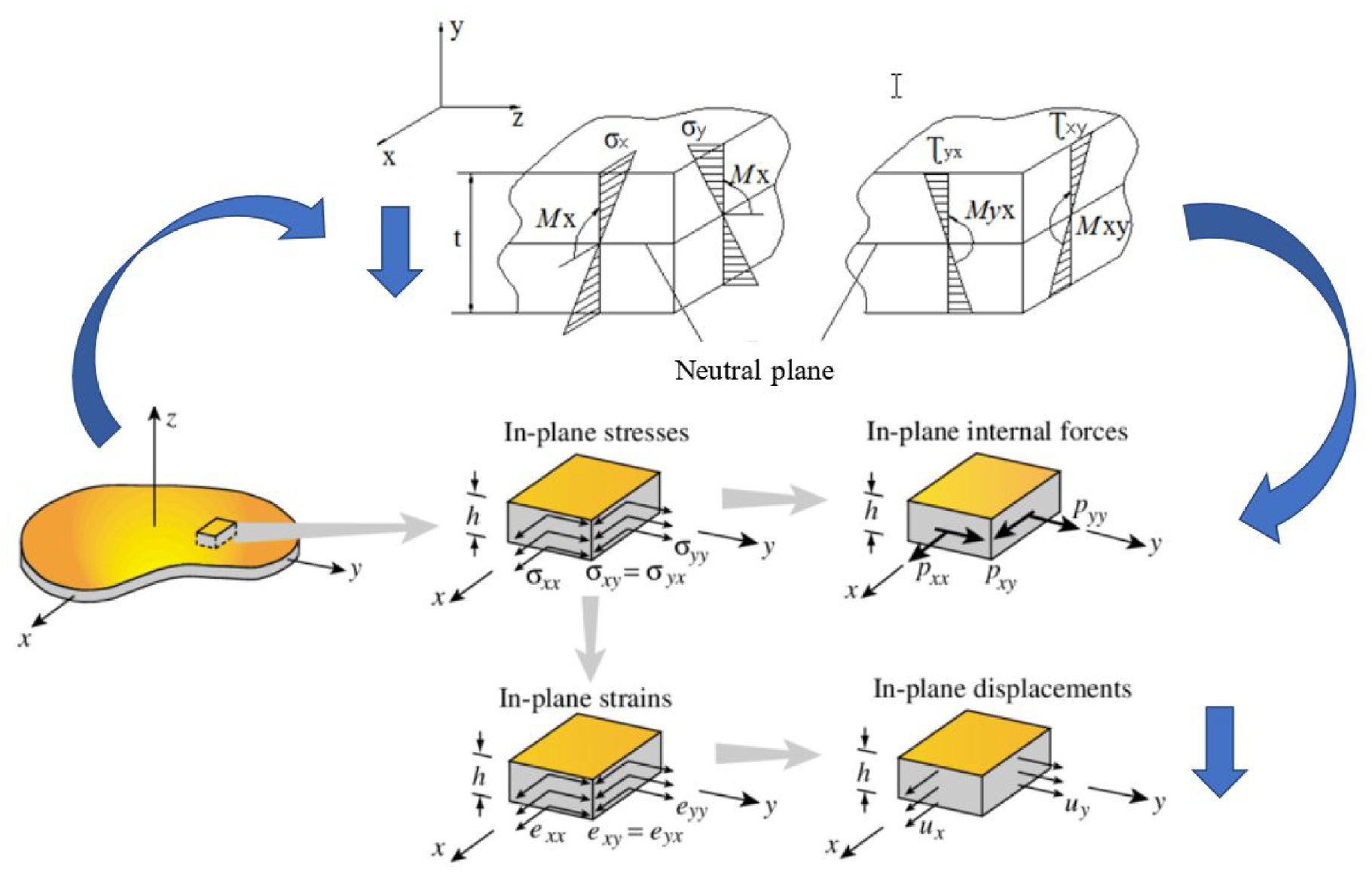
Stress on a thin plate element.

These stresses have created the bending moment M_x, M_y and the torque moment M_xy, M_yx on the plate’s cross section. They are defined as follows:

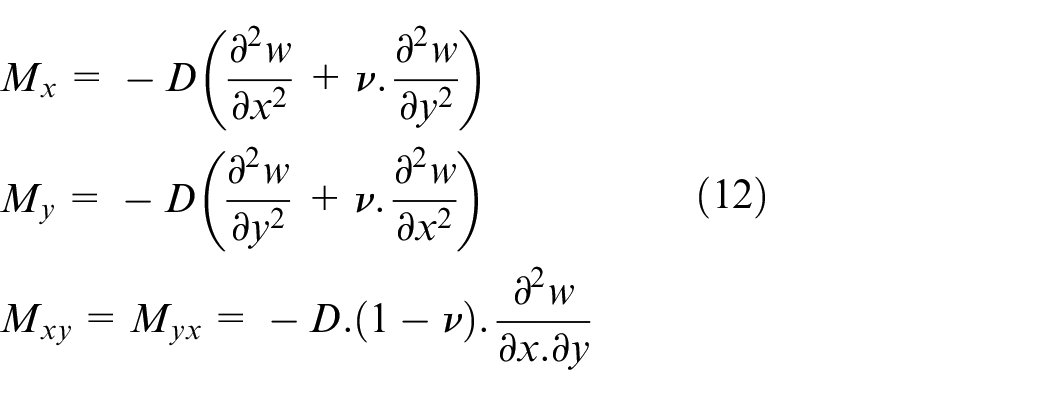
\begin{matrix} M_{x} = - D (\frac{\partial^{2} w}{\partial x^{2}} + ν . \frac{\partial^{2} w}{\partial y^{2}}) \\ M_{y} = - D (\frac{\partial^{2} w}{\partial y^{2}} + ν . \frac{\partial^{2} w}{\partial x^{2}}) \\ M_{xy} = M_{yx} = - D . (1 - ν) . \frac{\partial^{2} w}{\partial x . \partial y} \end{matrix}

(12)

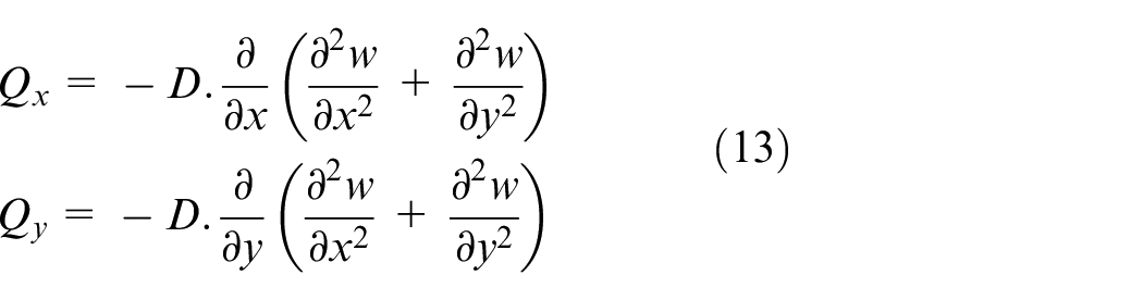
In which $D = \frac{E . h^{3}}{12 . (1 - ν^{2})}$ is called the cylindrical stiffness of the circular plate

Similarly, we can calculate the shear force in two perpendicular cross sections of the plate using the equation of Newton’s second law. Ignoring higher-order infinitesimals, we get:

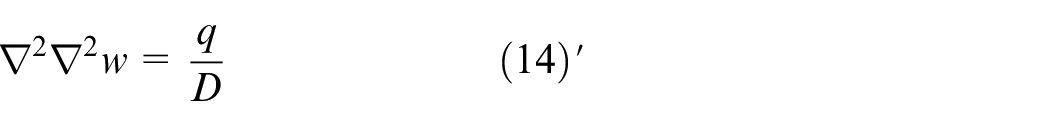
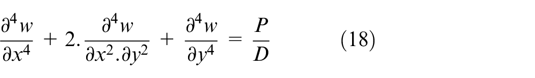
\begin{matrix} Q_{x} = - D . \frac{\partial}{\partial x} (\frac{\partial^{2} w}{\partial x^{2}} + \frac{\partial^{2} w}{\partial y^{2}}) \\ Q_{y} = - D . \frac{\partial}{\partial y} (\frac{\partial^{2} w}{\partial x^{2}} + \frac{\partial^{2} w}{\partial y^{2}}) \end{matrix}

(13)

The basic differential equation of the bent thin plate, commonly known as the Saint-Venant’s equation

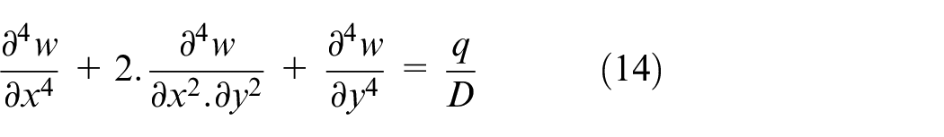
\frac{\partial^{4} w}{\partial x^{4}} + 2 . \frac{\partial^{4} w}{\partial x^{2} . \partial y^{2}} + \frac{\partial^{4} w}{\partial y^{4}} = \frac{q}{D}

(14)

or:

\nabla^{2} \nabla^{2} w = \frac{q}{D}

(14)′

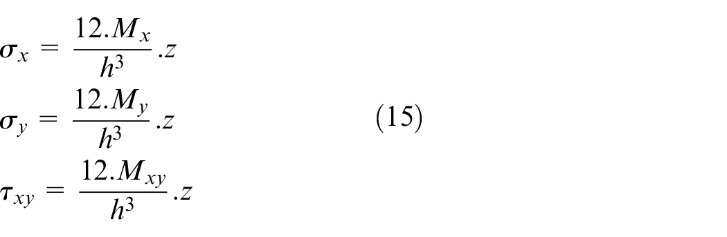
Substituting the moment and D expression into the stress formula, we get the concise stress expression as follows:

\begin{matrix} σ_{x} = \frac{12 . M_{x}}{h^{3}} . z \\ σ_{y} = \frac{12 . M_{y}}{h^{3}} . z \\ τ_{xy} = \frac{12 . M_{xy}}{h^{3}} . z \end{matrix}

(15)

Model’s mechanical characteristics

A thin circular plate mounted at the peripheral circumference is subjected to pressure uniformly distributed on its surface (P). Radius is R. We have the general equation of a circle with its center at the coordinate origin:

x^{2} + y^{2} = R^{2}

(16)

We use the inverse method to solve the problem of finding the deflection. Assuming that the plate’s deflection function has the form:

w (x, y) = w_{0} (\frac{x^{2}}{R^{2}} + \frac{y^{2}}{R^{2}} - 1)

(17)

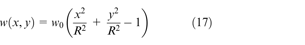
By substituting it into the basic differential equation of the thin plate (known as the Sophie Germain equation), we can obtain the maximum value of translocation

\frac{\partial^{4} w}{\partial x^{4}} + 2 . \frac{\partial^{4} w}{\partial x^{2} . \partial y^{2}} + \frac{\partial^{4} w}{\partial y^{4}} = \frac{P}{D}

(18)

Boundary conditions of the computational model on thin plates

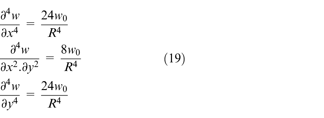
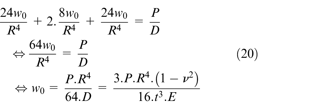
\begin{matrix} \frac{\partial^{4} w}{\partial x^{4}} = \frac{24 w_{0}}{R^{4}} \\ \frac{\partial^{4} w}{\partial x^{2} . \partial y^{2}} = \frac{8 w_{0}}{R^{4}} \\ \frac{\partial^{4} w}{\partial y^{4}} = \frac{24 w_{0}}{R^{4}} \end{matrix}

(19)

Then, the translocation of the thin plate is calculated as the expression (20)

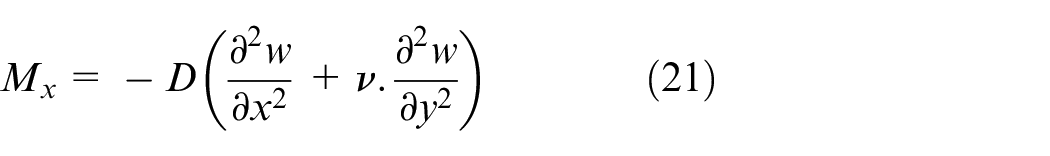
\begin{matrix} \frac{24 w_{0}}{R^{4}} + 2 . \frac{8 w_{0}}{R^{4}} + \frac{24 w_{0}}{R^{4}} = \frac{P}{D} \\ \Leftrightarrow \frac{64 w_{0}}{R^{4}} = \frac{P}{D} \\ \Leftrightarrow w_{0} = \frac{P . R^{4}}{64 . D} = \frac{3 . P . R^{4} . (1 - ν^{2})}{16 . t^{3} . E} \end{matrix}

(20)

Similar to translocation, the stress of the thin plate is determined through the bending moment M_x, M_y caused by the stress components. These moment components affect the differential elements of the thin plate through equation (21).

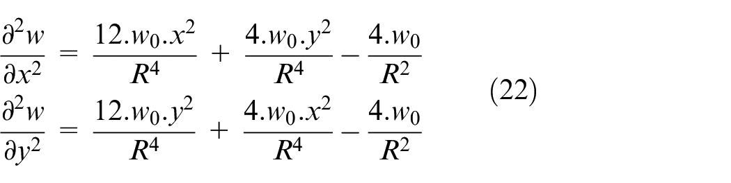
M_{x} = - D (\frac{\partial^{2} w}{\partial x^{2}} + ν . \frac{\partial^{2} w}{\partial y^{2}})

(21)

Conditions from differential equations are illustrated as equation (22)

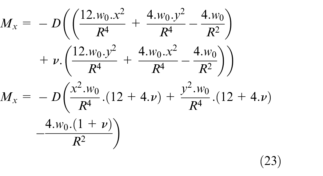
\begin{matrix} \frac{\partial^{2} w}{\partial x^{2}} = \frac{12 . w_{0} . x^{2}}{R^{4}} + \frac{4 . w_{0} . y^{2}}{R^{4}} - \frac{4 . w_{0}}{R^{2}} \\ \frac{\partial^{2} w}{\partial y^{2}} = \frac{12 . w_{0} . y^{2}}{R^{4}} + \frac{4 . w_{0} . x^{2}}{R^{4}} - \frac{4 . w_{0}}{R^{2}} \end{matrix}

(22)

Then, the moment impacts according to x direction of the thin plate demonstrated as equation (23)

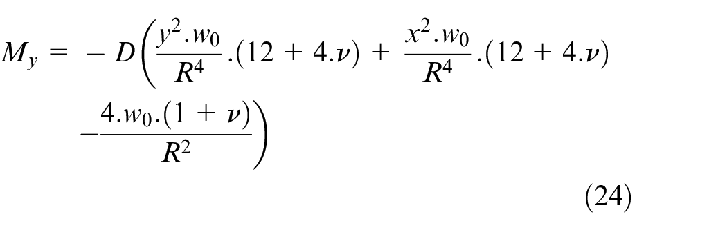
\begin{matrix} M_{x} = - D ((\frac{12 . w_{0} . x^{2}}{R^{4}} + \frac{4 . w_{0} . y^{2}}{R^{4}} - \frac{4 . w_{0}}{R^{2}}) \\ + ν . (\frac{12 . w_{0} . y^{2}}{R^{4}} + \frac{4 . w_{0} . x^{2}}{R^{4}} - \frac{4 . w_{0}}{R^{2}})) \\ M_{x} = - D (\frac{x^{2} . w_{0}}{R^{4}} . (12 + 4 . ν) + \frac{y^{2} . w_{0}}{R^{4}} . (12 + 4 . ν) \\ - \frac{4 . w_{0} . (1 + ν)}{R^{2}}) \end{matrix}

(23)

Then, the moment impacts according to direction y of the thin plate similar to moment acts according to direction x, illustrated as equation (24)

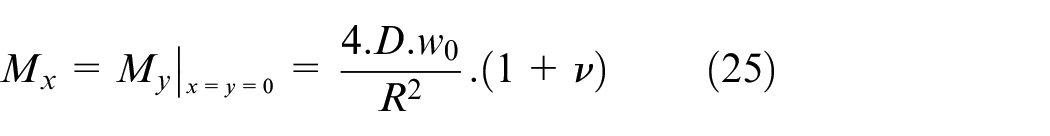
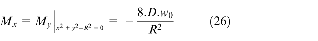
\begin{matrix} M_{y} = - D (\frac{y^{2} . w_{0}}{R^{4}} . (12 + 4 . ν) + \frac{x^{2} . w_{0}}{R^{4}} . (12 + 4 . ν) \\ - \frac{4 . w_{0} . (1 + ν)}{R^{2}}) \end{matrix}

(24)

Applying the thin plate’s boundary condition, the moments at the plate center and at the boundary are demonstrated as equations (25) and (26)

M_{x} = M_{y} |_{x = y = 0} = \frac{4 . D . w_{0}}{R^{2}} . (1 + ν)

(25)

M_{x} = M_{y} |_{x^{2} + y^{2} - R^{2} = 0} = - \frac{8 . D . w_{0}}{R^{2}}

(26)

We can determine the corresponding stress at the thin plate’s center and boundary

Building the measurement system by deep learning model

The water pressure sensing system in the pores consists of three parts: the sensing system, the signal acquisition system, and the data display system, as shown in Figure 8.

Figure 8.

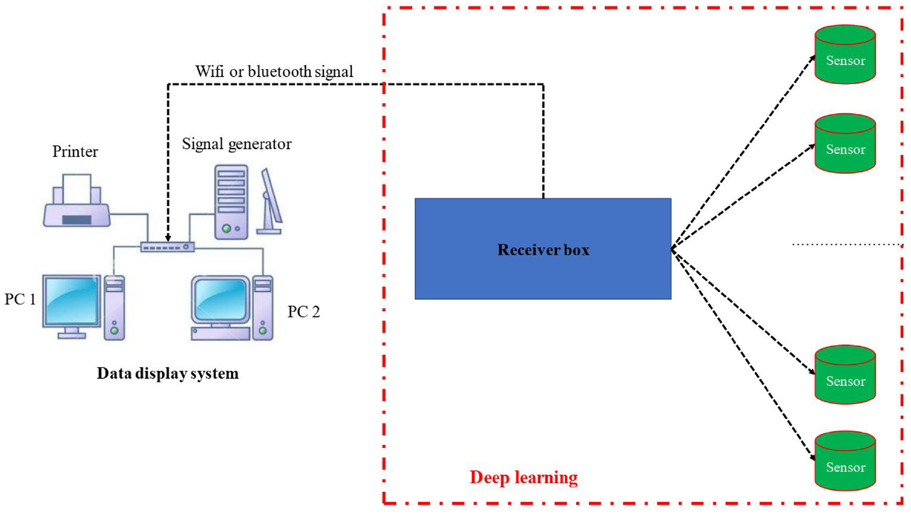
Measurement system model.

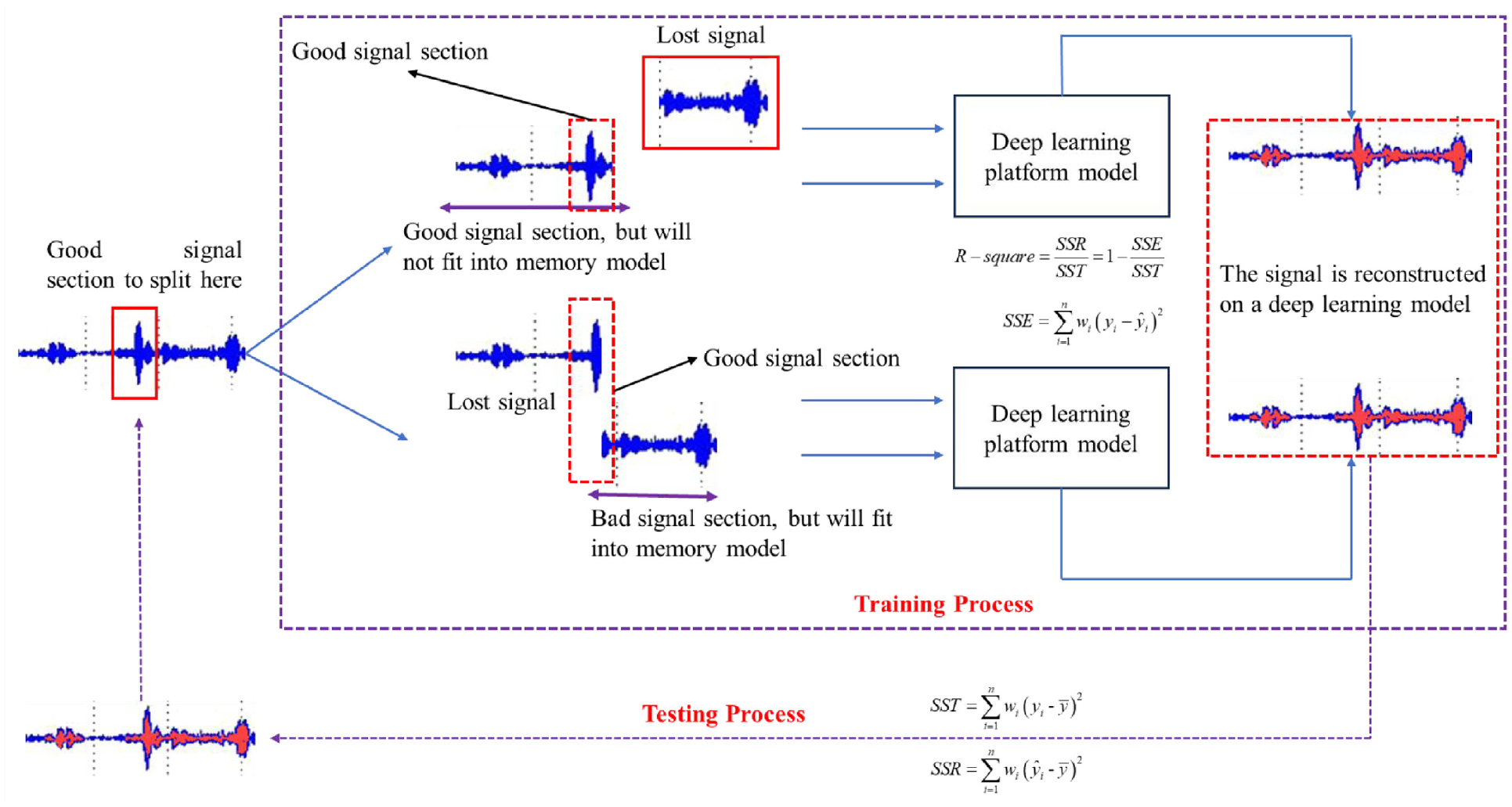
The manuscript presents a measurement model based on deep learning, designed to operate in complex and noisy environments during the measurement and data display process, as depicted in Figure 9(a) and (b). The model training process involves three steps:

Figure 9.

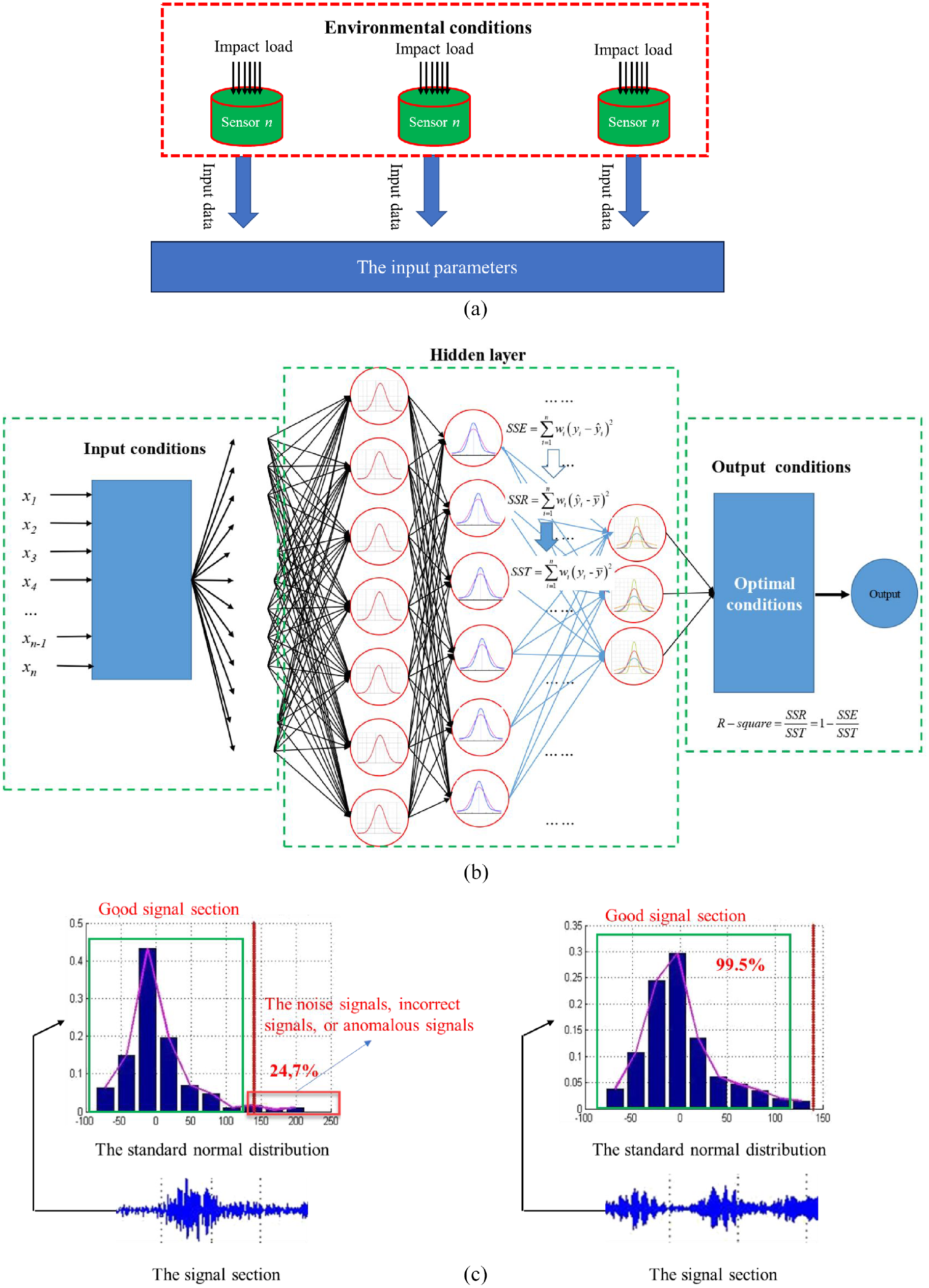
(a) The input parameters of the measurement system model, (b) data training model, and (c) advantages of the research model.

Step 1: Defining the input parameters. The input values are represented by a set of x_i values, where i ranges from 1 to n, obtained during a time interval t from the actual sensor operation.

Step 2: The training process, depicted in Figure 9(b), involves the use of n hidden layers, with each layer employing a training function represented by equation (27). In case of normalizing the quantitative $\frac{x - \bar{x}}{σ} = z$ , then z is called a standardized variable. Provided that the distribution of value z in the range N (0,1)

\begin{matrix} P (X \geq x) = \frac{1}{\sqrt{2 π σ}} \int_{x}^{\infty} \exp {- \frac{1}{2} {(\frac{x - \bar{x}}{σ})}^{2}} dx \\ P (X < x) = 1 - \frac{1}{\sqrt{2 π σ}} \int_{- \infty}^{x} \exp {- \frac{1}{2} {(\frac{x - \bar{x}}{σ})}^{2}} dx \end{matrix}

(27)

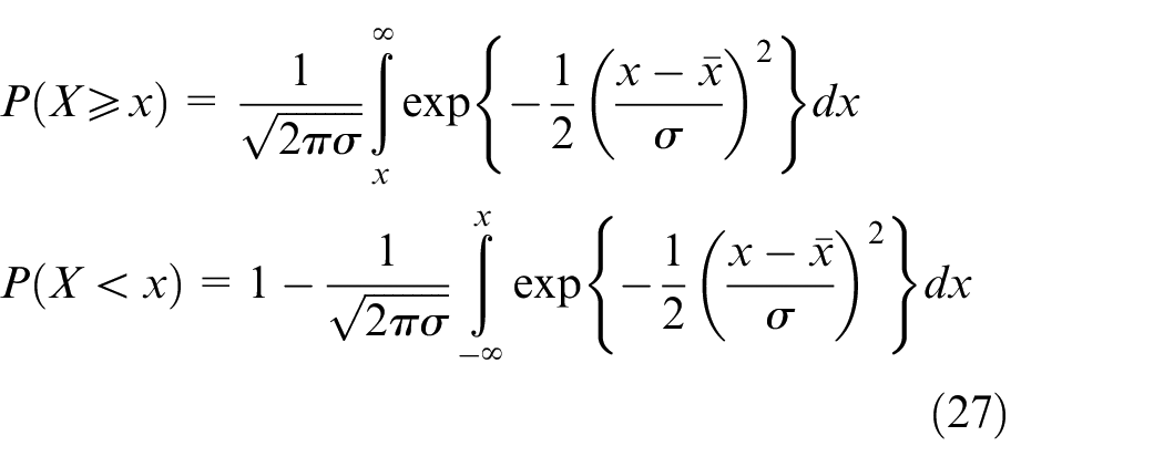
In equation (27), the model is trained based on the cumulative distribution function of the standard normal distribution. This model aims to eliminate noise signals, incorrect signals, or anomalous signals in the process of signal acquisition from the sensor. Some segments of noisy signals are removed during the experimentation, as depicted in Figure 9(c). Specifically, the noise signals are completely eliminated during the training process to enhance the efficiency of signal acquisition from the measuring sensor. This constitutes a novel aspect in the implementation of this research compared to other sensor groups currently available in the market.

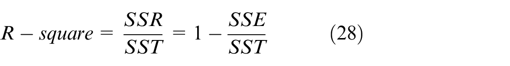
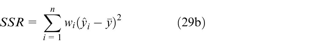
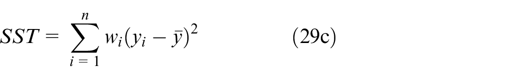
Step 3: The output parameter of the system is obtained by measuring the value at each duration after achieving the convergence value using equation (28), and calculating the sum of SSE deviation squares as shown in equation (29a), the sum of SSR regression squares as shown in equation (29b), and the sum of SST squares as shown in equation (29c), as illustrated in Figure 10.

R - square = \frac{SSR}{SST} = 1 - \frac{SSE}{SST}

(28)

SSE = \sum_{i = 1}^{n} w_{i} {(y_{i} - {\hat{y}}_{i})}^{2}

(29a)

SSR = \sum_{i = 1}^{n} w_{i} {({\hat{y}}_{i} - \bar{y})}^{2}

(29b)

SST = \sum_{i = 1}^{n} w_{i} {(y_{i} - \bar{y})}^{2}

(29c)

Figure 10.

Data acquisition model.

Fabrication designing

Assuming that the mechanical behavior of the elastic diaphragm is ideal, the design process for an elastic diaphragm to achieve an output voltage of e₀ = 3 mV/V when subjected to a pressure of p = 40.103 Pa on the surface involves the following steps:

The material for fabricating the elastic diaphragm is elastic and homogeneous.

Calculate the required deflection of the diaphragm using the following equation:

δ = \frac{P . R^{4}}{64 . t . E . (1 - v^{2})}

(30)

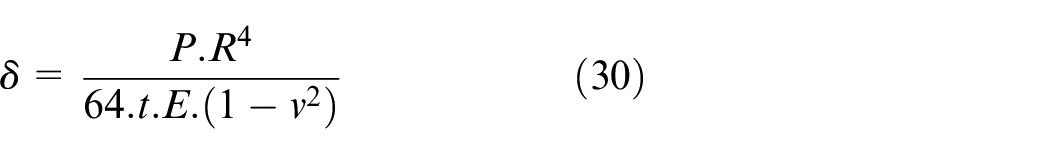
where δ is the deflection, P is the pressure, R is the radius of the diaphragm, t is the thickness of the diaphragm, E is the Young’s modulus of the diaphragm material, and v is the Poisson’s ratio of the diaphragm material.

Tính toán đ $\underset{\cdot}{\hat{o}}$ $nh \underset{\cdot}{a} y$ c $\overset{`}{\hat{a}}$ n thi $\overset{'}{\hat{e}}$ t c $\overset{'}{u}$ a màng ngăn b $\overset{'}{\overset{⌣}{a}}$ ng phu’o’ng trình sau:

S = \frac{e_{0} . V_exc}{δ . A}

(31)

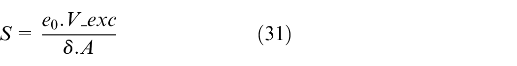
where S is the sensitivity, e₀ is the desired output voltage, V_exc is the excitation voltage, δ is the deflection, and A is the area of the diaphragm.

Determine the appropriate excitation voltage based on the sensitivity and the maximum output voltage of the signal reader.

Calculate the required thickness of the diaphragm using the following equation:

t = \frac{P . R^{4}}{64 . S . E . (1 - v^{2})}

(32)

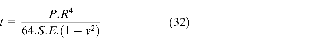
By following these steps, an elastic diaphragm can be designed to achieve the desired output voltage when subjected to a specific pressure. Use a signal reader with a signal interval in the range of interest. The problem is to design an elastic diaphragm that will produce an output voltage of e₀ = 3 mV/V when subjected to a pressure of p = 40.103 Pa acting on its surface.

Pressure diaphragm design

Let R be the radius of the elastic diaphragm, t be the thickness of the diaphragm, L be the thickness of the side wall, and h be the height of the side wall. We can represent the sensor as a 2D model, as shown in Figure 11.

Figure 11.

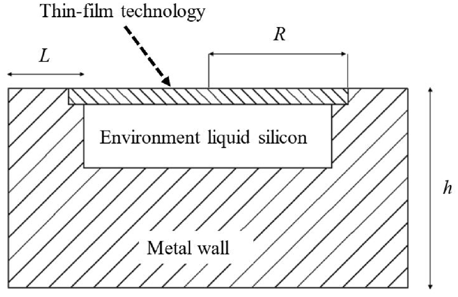
Geometric dimension of the elastic diaphragm.

We can see, the diaphragm’s deformation at the center and peripheral circumference has a large value in terms of magnitude, corresponding to the tensile deformation and the compressive deformation, the tensile and compressive deformation values are illustrated in the Figure 7 and demonstrated in equation (33).

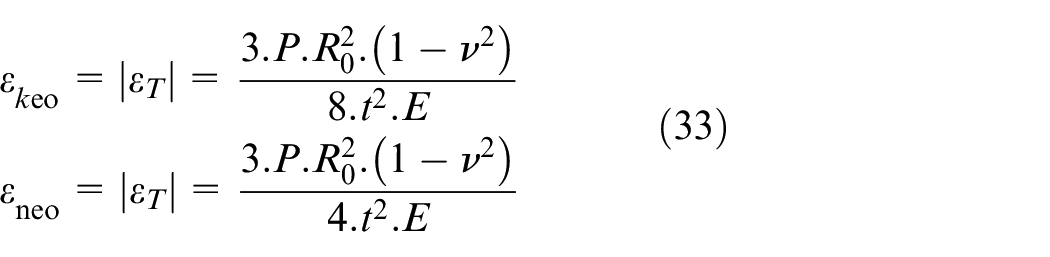
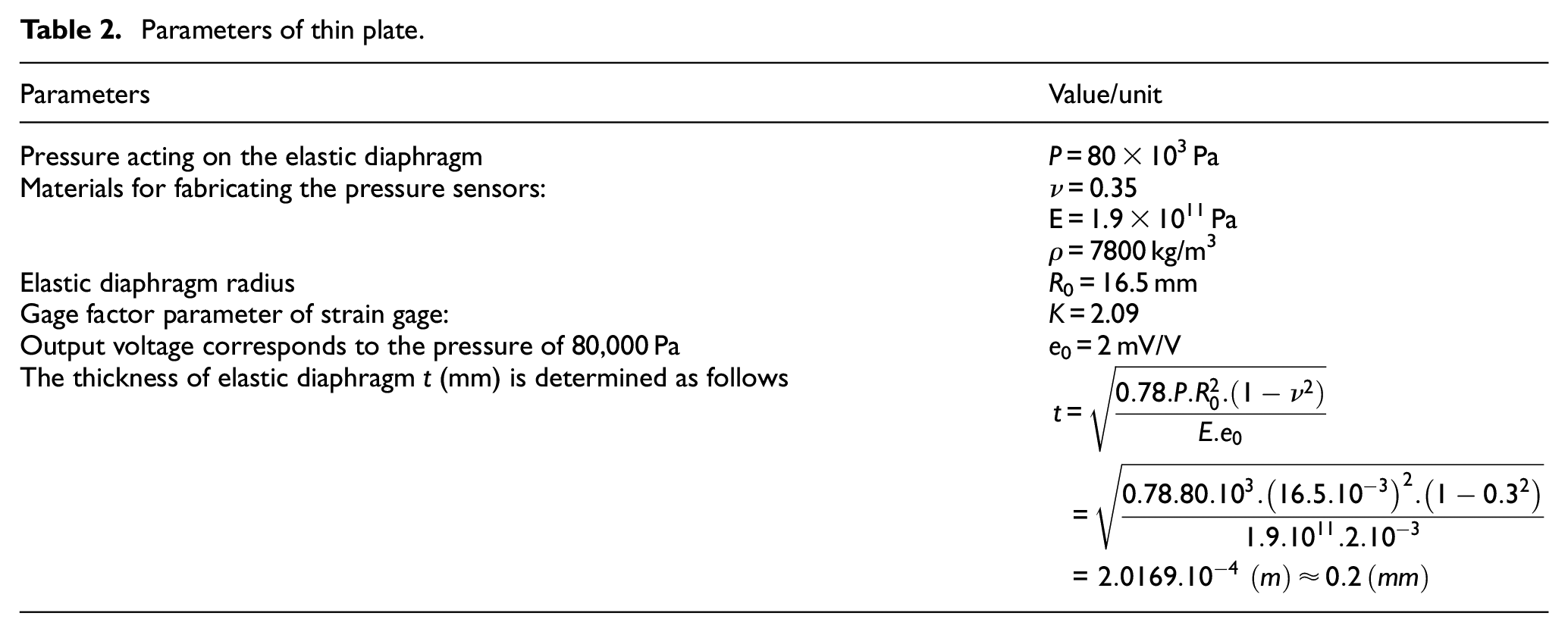
\begin{matrix} ε_{k e o} = | ε_{T} | = \frac{3 . P . R_{0}^{2} . (1 - ν^{2})}{8 . t^{2} . E} \\ ε_{n e o} = | ε_{T} | = \frac{3 . P . R_{0}^{2} . (1 - ν^{2})}{4 . t^{2} . E} \end{matrix}

(33)

Therefore, the resistance bridges need to be located in the area with the largest deformation in order for the strain gage sensor to operate most effectively. Thus, the preliminary radius of the elastic diaphragm that has been chosen must be at least greater than the strain gage outer diameter because a straight strain gage is used: R > R_{strain_gauge} = 5mm. The material parameters are shown in Table 2.

Table 2.

Parameters of thin plate.

Parameters	Value/unit
Pressure acting on the elastic diaphragm	P = 80 × 10³ Pa
Materials for fabricating the pressure sensors:	ν = 0.35
	E = 1.9 × 10¹¹ Pa
	ρ = 7800 kg/m³
Elastic diaphragm radius	R ₀ = 16.5 mm
Gage factor parameter of strain gage:	K = 2.09
Output voltage corresponds to the pressure of 80,000 Pa	e ₀ = 2 mV/V
The thickness of elastic diaphragm t (mm) is determined as follows	$\begin{matrix} t = \sqrt{\frac{0.78 . P . R_{0}^{2} . (1 - ν^{2})}{E . e_{0}}} \\ = \sqrt{\frac{{0.78.80.10}^{3} . {({16.5.10}^{- 3})}^{2} . (1 - {0.3}^{2})}{{1.9.10}^{11} {. 2.10}^{- 3}}} \\ = 2.0169 . 10^{- 4} (m) \approx 0.2 (mm) \end{matrix}$

Designing the pressure wall

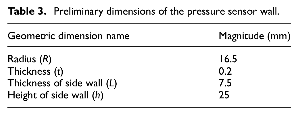
The thin plate is firmly attached to the peripheral circumference of the wall, as shown in Figure 8, to design the sensor wall according to the theory analyzed above. The deformation of the diaphragm is completely independent of the deformation of the side wall. Additionally, due to the thickness and material structure of the wall, deformation around the wall cannot occur. The requirement is: L > 30t, where t is the thickness of the elastic diaphragm. For example, if t = 0.2 mm, then L should be greater than 6 mm. Taking preliminary selection of wall thickness to connect to elastic plate with L = 7.5 mm. We choose h = 25 mm in order for the sensor to be complete and esthetic. Table 3 summarizes the preliminary dimensions of the calculated elastic diaphragm.

Table 3.

Preliminary dimensions of the pressure sensor wall.

Geometric dimension name	Magnitude (mm)
Radius (R)	16.5
Thickness (t)	0.2
Thickness of side wall (L)	7.5
Height of side wall (h)	25

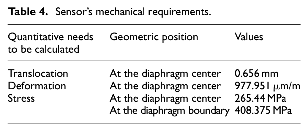
Then, the requirements must be achieved to ensure the sensor operation are shown in Table 4.

Table 4.

Sensor’s mechanical requirements.

Quantitative needs to be calculated	Geometric position	Values
Translocation	At the diaphragm center	0.656 mm
Deformation	At the diaphragm center	977.951 µm/m
Stress	At the diaphragm center	265.44 MPa
Stress	At the diaphragm boundary	408.375 MPa

Simulation of sensor durability and performance

We should use Abaqus software to simulate the sensor model and measure the water pressure in pores, as well as calculate mechanical values such as the sensor’s displacement, stress, and deformation while operating at the pile cap. Additionally, the water pressure acting on the thin plate will cause vibrations on the diaphragm, so the manuscript has surveyed the vibration process of the sensor system during operation. In the simulation, the shell element is used with a selected thickness of 0.0002 m, and the logical mapping mesh is divided into a size of 0.002 m, as shown in Figure 12(a). The boundary conditions, including the fixed constraint for the metal wall and the hydrostatic pressure acting on the thin plate, are shown in Figure 12(b).

Figure 12.

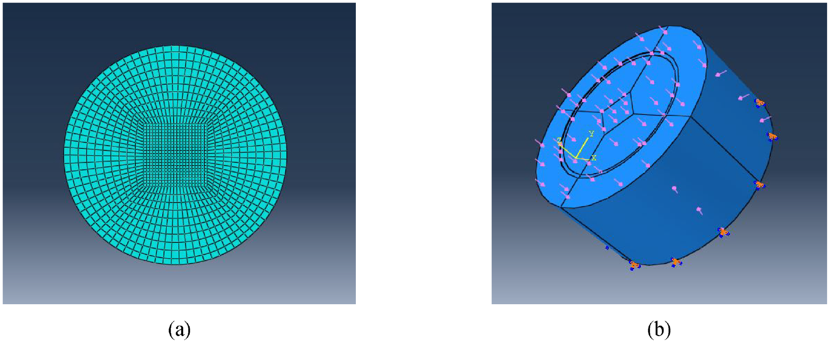
Sensor’s meshing model and force putting condition: (a) Meshing model of the sensor surface and (b) Force model of the sensor surface.

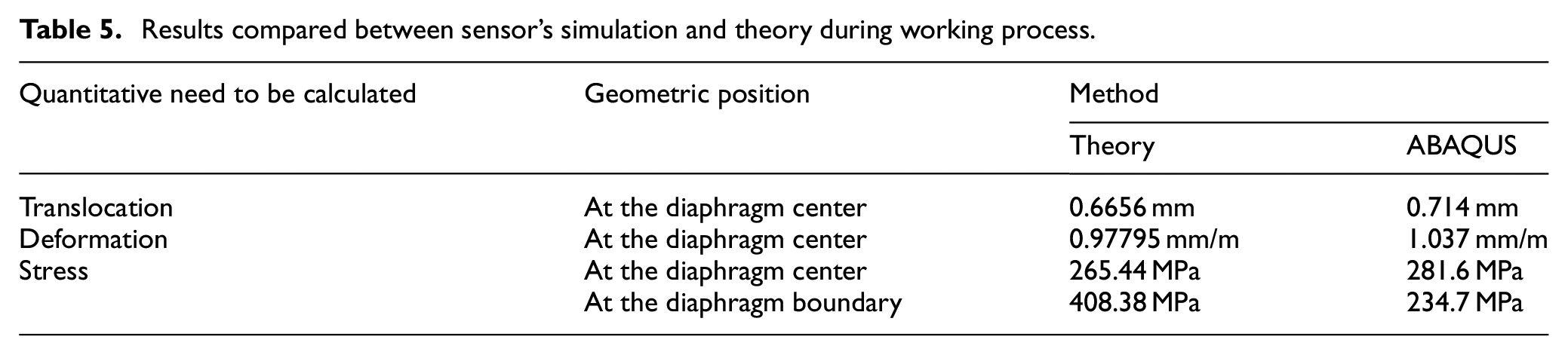
With the material parameters and load conditions as shown in Tables 1 –3, the translocation, deformation, and stress results of the sensor under actual working conditions are shown in Figure 13. The largest translocation occurs at the center of the diaphragm, with a magnitude of w_max = 0.714 mm. The deformation at the diaphragm center has a value of ϵ = 1.037 mm/m, and the stress at the diaphragm center has a value of σ = 281.6 MPa.

Figure 13.

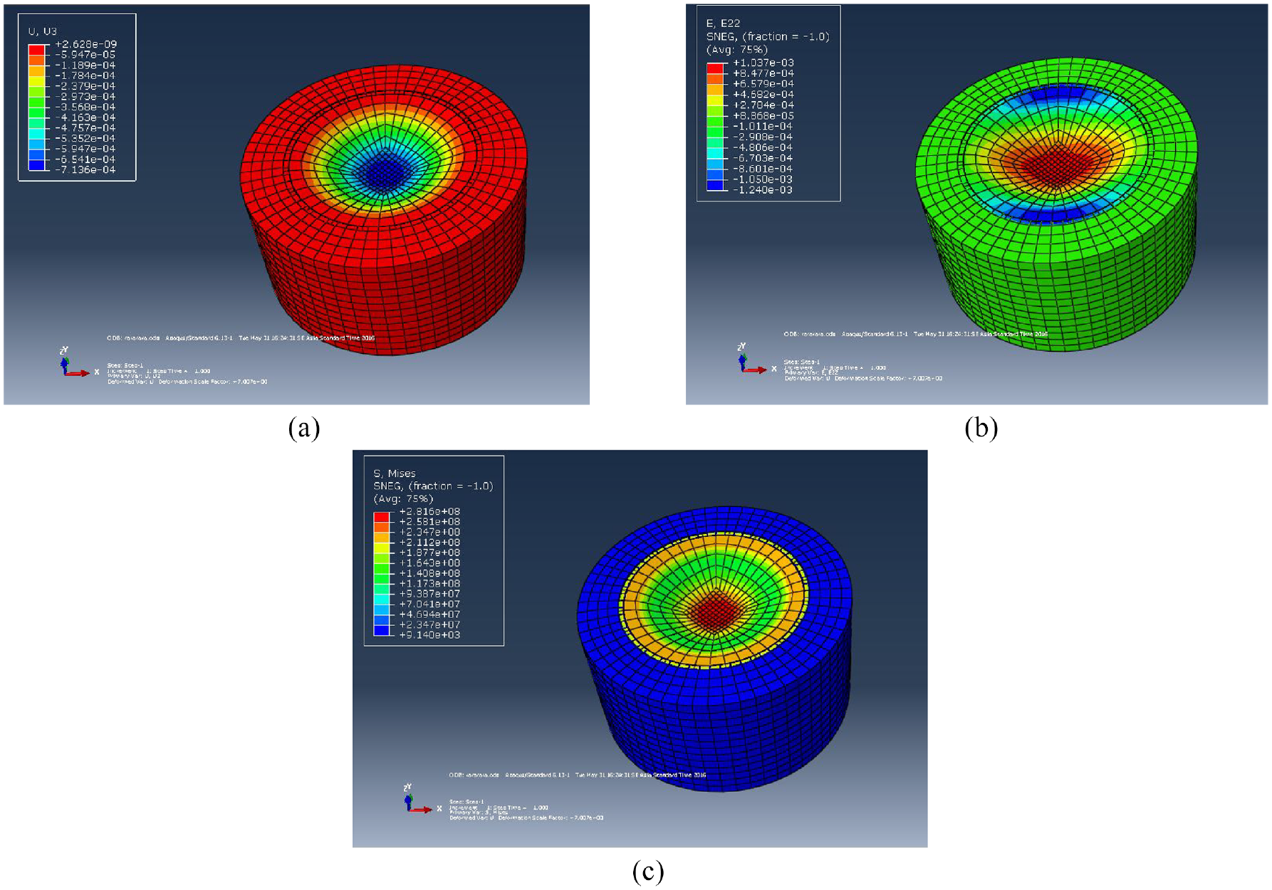
(a) Sensor’s translocation result, (b) sensor’s deformcation result, and (c) sensor’s maximum stress result.

Table 5 shows the comparison results between the mechanical parameters at the simulated internal diaphragm and the theoretical model.

Table 5.

Results compared between sensor’s simulation and theory during working process.

Quantitative need to be calculated	Geometric position	Method
Quantitative need to be calculated	Geometric position	Theory	ABAQUS
Translocation	At the diaphragm center	0.6656 mm	0.714 mm
Deformation	At the diaphragm center	0.97795 mm/m	1.037 mm/m
Stress	At the diaphragm center	265.44 MPa	281.6 MPa
Stress	At the diaphragm boundary	408.38 MPa	234.7 MPa

The vibration process of the thin plate is illustrated in Table 6, in which the vibration patterns are surveyed from mode 1 to mode 10. This means the limitation of this study lies in the design, manufacturing of sensors only enduring pressure distributed along the sensor membrane while neglecting forces acting on other directions. Therefore, the simulation process always assumes that the edges (boundaries) of the sensor are in an absolutely rigid state. The diaphragm can vibrate from mode 1 to higher modes due to the action of hydrostatic pressure. The manuscript has surveyed all different types of vibrations to ensure the sensor operates safely and stably in the working environment at the pile cap. It can be seen that the elastic diaphragm operates stably even in high vibration modes. Because higher vibration modes make the sensor model more robust. Typically, previous studies only tested durability from vibration modes 5 to 6. However, given the working environment characteristics of this type of sensor, the research has extended durability testing through the 10th vibration mode. This enhances the durability and stability of the sensor under real-world conditions.

Table 6.

Sensor’s vibration modes of the elastic diaphragm.

Mode 1: f = 1,784.0 rad/s	Mode 2: f = 3,784.7 rad/s
Mode 3: f = 3,787.5 rad/s	Mode 4: f = 6,214.4 rad/s
Mode 5: f = 6,333.0 rad/s	Mode 6: f = 7,305.1 rad/s
Mode 7: f = 9,24.8 rad/s	Mode 8: f = 9,253.3 rad/s
Mode 9: f = 11,421 rad/s	Mode 10: f = 11,427 rad/s

Experiment and standardization

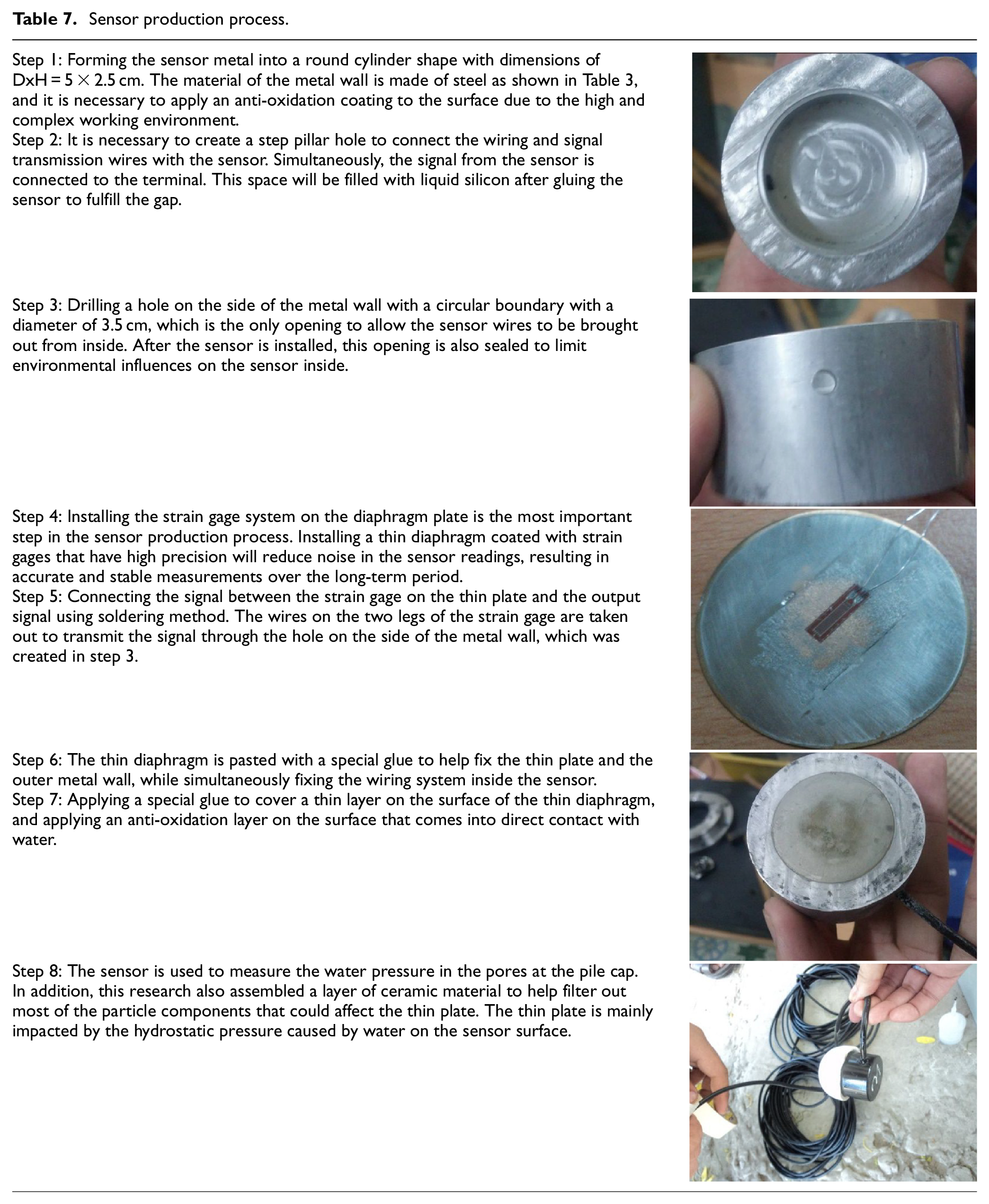
Similar to the simulation process and research limitations described in Table 6, the sensor manufacturing process will be outlined in Table 7, where the outer casing of the sensor is fabricated using hard metals and processed through advanced technology machining models. This ensures absolute rigidity for the sensor when operating in environments with various external forces. In contrast to the outer casing of the sensor, the sensor membrane model is manufactured using thin membrane models to absorb all external forces acting on the membrane. The sensor production process is presented in Table 7, which consists of seven steps. The sensor details are manufactured using CNC machining methods to ensure high accuracy during operation.

Table 7.

Sensor production process.

Step 1: Forming the sensor metal into a round cylinder shape with dimensions of DxH = 5 × 2.5 cm. The material of the metal wall is made of steel as shown in Table 3, and it is necessary to apply an anti-oxidation coating to the surface due to the high and complex working environment.
Step 2: It is necessary to create a step pillar hole to connect the wiring and signal transmission wires with the sensor. Simultaneously, the signal from the sensor is connected to the terminal. This space will be filled with liquid silicon after gluing the sensor to fulfill the gap.
Step 3: Drilling a hole on the side of the metal wall with a circular boundary with a diameter of 3.5 cm, which is the only opening to allow the sensor wires to be brought out from inside. After the sensor is installed, this opening is also sealed to limit environmental influences on the sensor inside.
Step 4: Installing the strain gage system on the diaphragm plate is the most important step in the sensor production process. Installing a thin diaphragm coated with strain gages that have high precision will reduce noise in the sensor readings, resulting in accurate and stable measurements over the long-term period.
Step 5: Connecting the signal between the strain gage on the thin plate and the output signal using soldering method. The wires on the two legs of the strain gage are taken out to transmit the signal through the hole on the side of the metal wall, which was created in step 3.
Step 6: The thin diaphragm is pasted with a special glue to help fix the thin plate and the outer metal wall, while simultaneously fixing the wiring system inside the sensor.
Step 7: Applying a special glue to cover a thin layer on the surface of the thin diaphragm, and applying an anti-oxidation layer on the surface that comes into direct contact with water.
Step 8: The sensor is used to measure the water pressure in the pores at the pile cap. In addition, this research also assembled a layer of ceramic material to help filter out most of the particle components that could affect the thin plate. The thin plate is mainly impacted by the hydrostatic pressure caused by water on the sensor surface.

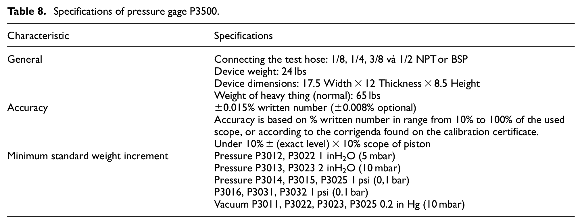
Given the constraints on experimental equipment conditions and the characteristics of the measurement sensor model, although the measurement device model exhibits anisotropy, the sensor design process in this draft is consistently based on a spherical state. Due to the symmetry of the spherical model, under the influence of external forces, deformation remains uniform in all directions and converges toward the center of the sensor. Consequently, the results of this measurement sensor model remain stable, and the level of stability is reflected as shown in Table 9. An experiment was conducted using the sensor model to compare the measured results with the simulation process on Abaqus software and the P300 pressure gage with technical characteristics as shown in Table 8. The results of the different methods are compared and demonstrated in Table 9.

Table 8.

Specifications of pressure gage P3500.

Characteristic	Specifications
General	Connecting the test hose: 1/8, 1/4, 3/8 và 1/2 NPT or BSP
	Device weight: 24 lbs
	Device dimensions: 17.5 Width × 12 Thickness × 8.5 Height
	Weight of heavy thing (normal): 65 lbs
Accuracy	±0.015% written number (±0.008% optional)
	Accuracy is based on % written number in range from 10% to 100% of the used scope, or according to the corrigenda found on the calibration certificate.
	Under 10% ± (exact level) × 10% scope of piston
Minimum standard weight increment	Pressure P3012, P3022 1 inH₂O (5 mbar)
	Pressure P3013, P3023 2 inH₂O (10 mbar)
	Pressure P3014, P3015, P3025 1 psi (0,1 bar)
	P3016, P3031, P3032 1 psi (0.1 bar)
	Vacuum P3011, P3022, P3023, P3025 0.2 in Hg (10 mbar)

Table 9.

Comparison of sensor system’s experimental measurement results.

Meter	Present				Theory	Abaqus	P3500
Pressure (pa)	Test 1	Test 2	Test 3	Error value (%)	Theory	Abaqus	P3500
0	0	0	0	0.000	0	0	0
3.924	60	62	59	0.607	66.972	59.982	61.250
7.848	104	103	102	0.532	93.944	101.964	102.121
11.772	140	140	142	0.186	140.916	142.946	142.045
15.696	201	202	201	0.301	187.888	203.928	204.148
19.620	334	331	333	0.164	334.861	334.910	333.741
23.544	382	381	380	0.198	381,833	385,893	382.142
27.468	440	442	443	0.157	438.805	446.875	442.543
31.392	477	479	477	0.226	475.777	477.857	477.985
35.316	499	495	496	0.238	492.749	498.839	496.972
39.240	528	524	526	1.859	524.722	520.821	525.622

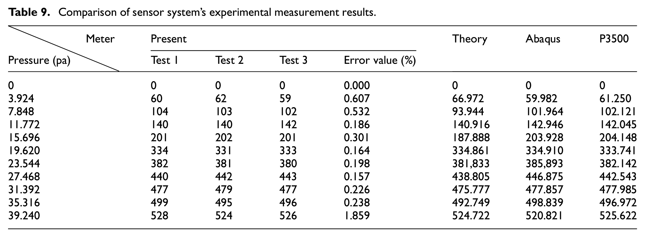
The standardized experimental data shown in Table 9 demonstrate that the sensor system provides highly accurate measurements, despite being subjected to complex and random loads. However, significant differences between the measured values and theoretical models remain due to imperfections in the production process and material parameters. The experiment was conducted in a flooded environment with a pile driving model consisting of 16 different piles. Two cases were considered: In case 1, the water pressure in the pores was measured at the outer pile foundation (M), which is subjected to a smaller load than the inner foundation (F). The water pressure evaluation results for this model are shown in Figure 14.

Figure 14.

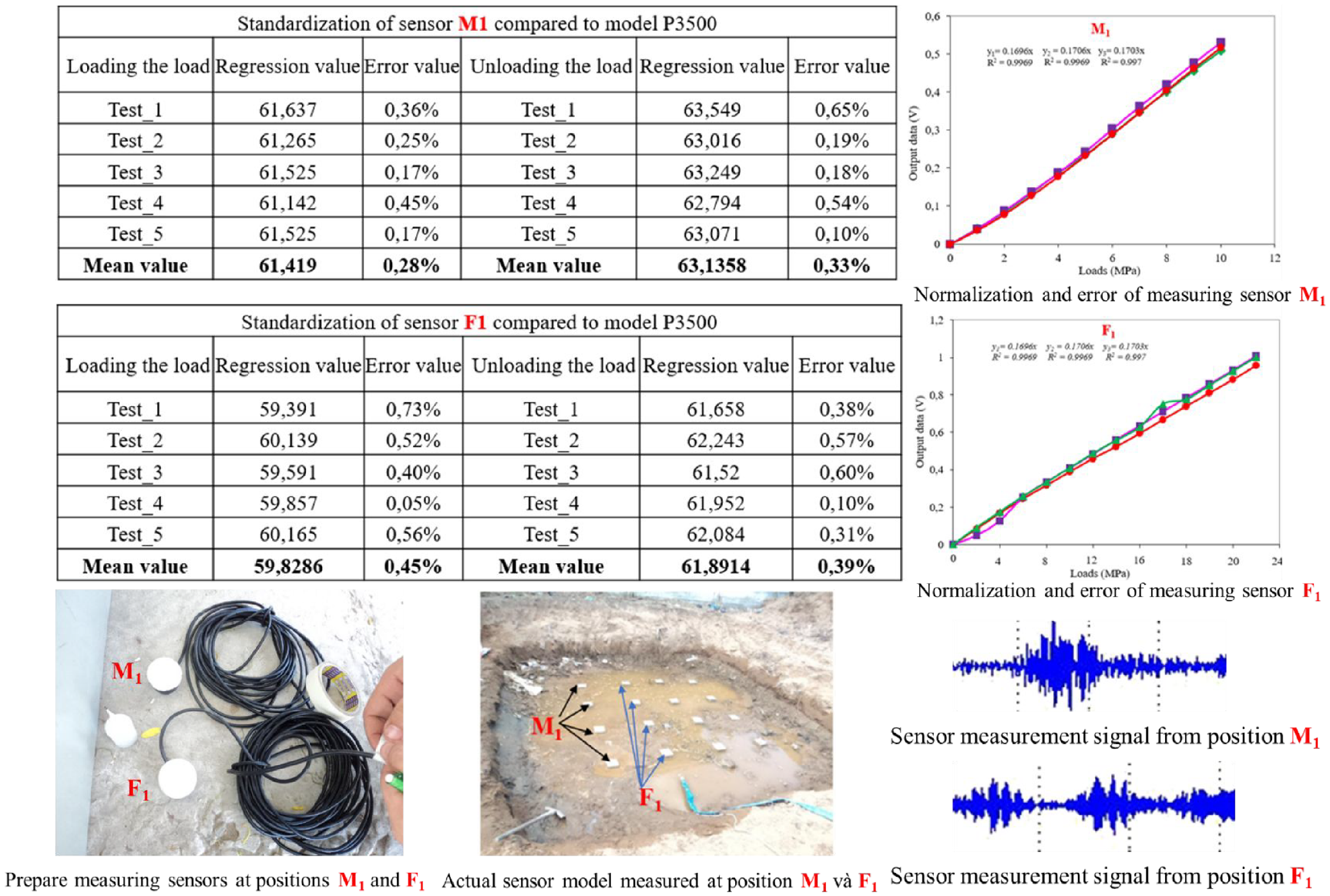
Model of water pressure measurement in pores at the pile foundation cap.

The sensor system for measuring water pressure in the pores at the geotextile layers is shown in Figure 15 at two locations K₁ and K₂. The results show that the sensor system operates with high stability under various working conditions and different types of loads. The training coefficient R₂ consistently reaches a value equivalent to 1. This indicates that the sensor system can meet the necessary requirements for the measurement process at the pile foundation cap during construction.

Figure 15.

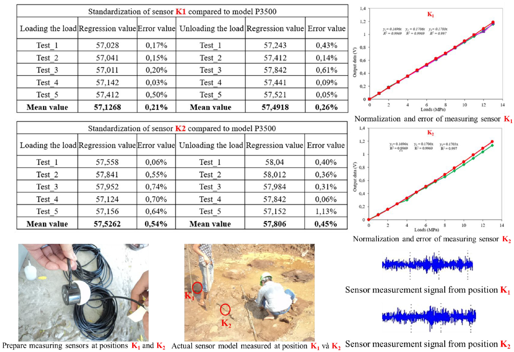
Model of water pressure measurement in pores at the high-tech fabric layer.

Conclusion

The manuscript introduces a novel sensor system designed and manufactured to accurately measure water pressure within pores, utilizing strain gage technology alongside deep learning algorithms for data processing and display. The development of such a pressure sensor entails extensive investment in time, resources, and materials. This study is particularly focused on monitoring water pressure within pores at a pile foundation cap. The sensor is engineered to withstand the harsh conditions of deep-water environments, ensuring durability, resistance to oxidation, and operational stability. The research extends beyond mere fabrication to encompass comprehensive experimentation and analysis, yielding several key findings:

- Utilizing numerical simulation software, calculations are conducted and cross-verified with analytical and experimental data to establish a robust dataset. The obtained results are then normalized and fed into a deep learning model, resulting in significantly enhanced accuracy compared to conventional systems.

- The study introduces a novel data acquisition model based on deep learning algorithms, aimed at optimizing output values. This model is particularly beneficial in environments characterized by high noise and random loads, ensuring stable and precise signal acquisition. Input values undergo normalization and rigorous training to optimize the output data system.

- The sensor system undergoes rigorous testing in real-world working conditions, demonstrating exceptional stability and efficiency in signal acquisition. Furthermore, the manuscript proposes the development of various sensor models to accommodate diverse measurement scenarios, suggesting further research to explore additional measurement statuses and models, thereby maximizing the system’s operational capacity.

Footnotes

Declaration of conflicting interests

The author(s) declared no potential conflicts of interest with respect to the research, authorship, and/or publication of this article.

Funding

The author(s) received no financial support for the research, authorship, and/or publication of this article.

ORCID iD

Thanh Q Nguyen

Data availability statement

All data generated or analysed during this study are included in this published article (and its supplementary information files).

References

Xia

Yang

Wang

, et al. Internet of things. Int J Commun Syst 2012; 25(9): 1101–1102.

Hozdić

Smart factory for industry 4.0: a review. Int J Mod Manuf Technol 2015; 7(1): 28–35.

Dincer

Bruch

Costa-Rama

, et al. Disposable sensors in diagnostics, food, and environmental monitoring. Adv Mater 2019; 31(30): 1806739.

Munirathinam

. Industry 4.0: industrial internet of things (IIOT). Adv Comput 2020; 117(1): 129–164.

Abbasi

Islam

Shaikh

ZA.

A review of wireless sensors and networks’ applications in agriculture. Comput Stand Interfaces 2014; 36(2): 263–270.

Thorn

Johansen

Hammer

EA.

Recent developments in three-phase flow measurement. Meas Sci Technol 1997; 8(7): 691–701.

Sood

Kaur

Lenka

Design and development of automatic water flowmeter. Int J Comput Sci Eng Appl 2013; 3(3): 49–59.

Yan

Mass flow measurement of bulk solids in pneumatic pipelines. Meas Sci Technol 1996; 7(12): 1687–1706.

Yang

Xie

, et al. Gas/oil/water flow measurement by electrical capacitance tomography. Meas Sci Technol 2013; 24(7): 074001.

10.

Pasierb

Rekas

Solid-state potentiometric gas sensors—current status and future trends. J Solid State Electrochem 2009; 13: 3–25.

11.

Yan

Byrne

Woodhead

, et al. Velocity measurement of pneumatically conveyed solids using electrodynamic sensors. Meas Sci Technol 1995; 6(5): 515–537.

12.

, et al. Progress and trend of sensor technology for on-line oil monitoring. Sci China Technol Sci 2013; 56: 2914–2926.

13.

Helton

Ratner

Wisniewski

NA.

Biomechanics of the sensor-tissue interface—effects of motion, pressure, and design on sensor performance and the foreign body response—part I: theoretical framework. J Diabetes Sci Technol 2011; 5(3): 632–646.

14.

Zhao

Liu

, et al. Development and application of resistance strain force sensors. Sensors 2020; 20(20): 5826.

15.

Chathuranga

Wang

Noh

, et al. Magnetic and mechanical modeling of a soft three-axis force sensor. IEEE Sens J 2016; 16(13): 5298–5307.

16.

Maddipatla

Zhang

Bose

, et al. A polyimide based force sensor fabricated using additive screen-printing process for flexible electronics. IEEE Access 2020; 8: 207813–207821.

17.

Fiorillo

Critello

Pullano

SA.

Theory, technology and applications of piezoresistive sensors: a review. Sens Actuators A Phys 2018; 281: 156–175.

18.

Kumar

Pant

BD.

Design principles and considerations for the ‘ideal’ silicon piezoresistive pressure sensor: a focused review. Microsyst Technol 2014; 20: 1213–1247.

19.

Meti

Balavald

Sheeparmatti

BG.

MEMS piezoresistive pressure sensor: a survey. Int J Eng Res Appl 2016; 6(4): 23–31.

20.

Zhang

Liu

Guo

, et al. Design of the MEMS piezoresistive electronic heart sound sensor. Sensors 2016; 16(11): 1728.

21.

Golby

Advances in inductive position sensor technology. Sens Rev 2010; 30(2): 142–147.

22.

George

Zangl

Bretterklieber

, et al. A combined inductive–capacitive proximity sensor for seat occupancy detection. IEEE Trans Instrum Meas 2010; 59(5): 1463–1470.

23.

Fericean

Droxler

New noncontacting inductive analog proximity and inductive linear displacement sensors for industrial automation. IEEE Sens J 2007; 7(11): 1538–1545.

24.

Djuric

SM.

Performance analysis of a planar displacement sensor with inductive spiral coils. IEEE Trans Magn 2014; 50(4): 1–4.

25.

Puers

Capacitive sensors: when and how to use them. Sens Actuators A Phys 1993; 37-38: 93–105.

26.

Brasseur

Design rules for robust capacitive sensors. IEEE Trans Instrum Meas 2003; 52(4): 1261–1265.

27.

Luo

RC.

Design and implementation of capacitive proximity sensor using microelectromechanical systems technology. IEEE Trans Ind Electron 1998; 45(6): 886–894.

28.

Ernst

Streule

Schmitt

, et al. A capacitive sensor for non-contact nanoliter droplet detection. Sens Actuators A Phys 2009; 153(1): 57–63.

29.

Jiao

Egbe

Xie

, et al. Piezoelectric sensing techniques in structural health monitoring: a state-of-the-art review. Sensors 2020; 20(13): 3730.

30.

Rupitsch

. “Piezoelectric sensors and actuators,” simulation of piezoelectric sensor and actuator devices. In: Piezoelectric sensors and actuators. Topics in mining, metallurgy and materials engineering. Vol. 1. 2019, pp.83–126. Berlin/Heidelberg, Germany: Springer Berlin Heidelberg.

31.

Zhou

Khaliq

Tang

, et al. Simulation and design of piezoelectric microcantilever chemical sensors. Sens Actuators A Phys 2005; 125(1): 69–75.

32.

Tianze

Xia

Chuan

, et al. Analysis of the characteristics of piezoelectric sensor and research of its application. In: 18th IEEE international symposium on the applications of ferroelectrics, 2009.

33.

Sessler

GM.

Acoustic sensors. Sens Actuators A Phys 1991; 26(1–3): 323–330.

34.

Wang

Xiong

, et al. MEMS-based thermoelectric infrared sensors: a review. Front Mech Eng 2017; 12: 557–566.

35.

Jaeggi

Baltes

Moser

Thermoelectric AC power sensor by CMOS technology. IEEE Electron Device Lett 1992; 13(7): 366–368.

36.

Milanovic

Gaitan

Bowen

, et al. Thermoelectric power sensor for microwave applications by commercial CMOS fabrication. IEEE Electron Device Lett 1997; 18(9): 450–452.

37.

Wang

Liao

Liu

A thermoelectric power sensor and its package based on MEMS technology. J Microelectromech Syst 2012; 21(1): 121–131.

38.

Kaushik

Nance

Ahuja

. A review of the role of acoustic sensors in the modern battlefield. In: 11th AIAA/CEAS aeroacoustics conference, 2005.

39.

Katardjiev

Yantchev

Recent developments in thin film electro-acoustic technology for biosensor applications. Vacuum 2012; 86(5): 520–531.

40.

Van Parijs

Clark

Sousa-Lima

, et al. Management and research applications of real-time and archival passive acoustic sensors over varying temporal and spatial scales. Mar Ecol Prog Ser 2009; 395: 21–36.

41.

Hempel

Nezich

Kong

, et al. A novel class of strain gauges based on layered percolative films of 2D materials. Nano Lett 2012; 12(11): 5714–5718.

42.

Lei

Will

HA.

Thin-film thermocouples and strain-gauge technologies for engine applications. Sens Actuators A Phys 1998; 65(2-3): 187–193.

43.

Giorgino

Tormene

Lorussi

, et al. Sensor evaluation for wearable strain gauges in neurological rehabilitation. IEEE Trans Neural Syst Rehabil Eng 2009; 17(4): 409–415.

44.

Maiwald

Werner

Zoellmer

, et al. INKtelligent printed strain gauges. Sens Actuators A Phys 2010; 162(2): 198–201.

45.

Stauffer

Zhang

Tybrandt

, et al. Soft electronic strain sensor with chipless wireless readout: toward real-time monitoring of bladder volume. Adv Mater Technol 2018; 3(6): 1800031.

46.

Choi

Kim

, et al. Highly stretchable, hysteresis-free ionic liquid-based strain sensor for precise human motion monitoring. ACS Appl Mater Interfaces 2017; 9(2): 1770–1780.

47.

Agarwala

Goh

Yap

, et al. Development of bendable strain sensor with embedded microchannels using 3D printing. Sens Actuators A Phys 2017; 263: 593–599.

48.

Yao

Meng

Jin

, et al. Full-field deformation measurement of fiber composite pressure vessel using digital speckle correlation method. Polym Test 2005; 24(2): 245–251.

49.

Ohno

Naruse

Kihara

, et al. Industrial applications of the BOTDR optical fiber strain sensor. Opt Fiber Technol 2001; 7(1): 45–64.

50.

Cerracchio

Gherlone

Tessler

Real-time displacement monitoring of a composite stiffened panel subjected to mechanical and thermal loads. Meccanica 2015; 50: 2487–2496.

51.

Schajer

GS.

Hole-drilling residual stress measurements at 75: origins, advances, opportunities. Exp Mech 2010; 50: 245–253.

52.

Sellnau

Matekunas

Battiston

, et al. Cylinder-pressure-based engine control using pressure-ratio-management and low-cost non-intrusive cylinder pressure sensors. SAE Transactions 2020; 1: 899–918.

53.

Choi

Park

Won

, et al. Soft inductive coil spring strain sensor integrated with SMA spring bundle actuator. Sensors 2021; 21(7): 2304.

54.

Praetorius

Spring

KR.

The renal cell primary cilium functions as a flow sensor. Curr Opin Nephrol Hypertens 2003; 12(5): 517–520.

55.

Wan

Eisenman

Campbell

, et al. Siphon: overload traffic management using multi-radio virtual sinks in sensor networks. In: Proceedings of the 3rd international conference on Embedded networked sensor systems, 2005.

56.

Kurtom

Magram

Siphon regulatory devices: their role in the treatment of hydrocephalus. Neurosurg Focus 2007; 22(4): E5–E8.

57.

Leal-Junior

Marques

Diaphragm-embedded optical fiber sensors: a review and tutorial. IEEE Sens J 2021; 21(11): 12719–12733.

58.

Yang

Zhang

, et al. An fbg pressure sensor based on spring-diaphragm elastic structure for ultimate pressure detection. IEEE Sens J 2022; 22(3): 2213–2220.

59.

Zhou

ZG.

Representation-learning-based CNN for intelligent attack localization and recovery of cyber-physical power systems. IEEE Trans Neural Netw Learn Syst 2024; 35: 6145–6155.

60.

Huang

Differential evolution-based three stage dynamic cyber-attack of cyber-physical power systems. IEEE/ASME Trans Mechatron 2023; 28(2): 1137–1148.

61.

Vasoya

NH.

Revolutionizing nano materials processing through IoT-AI integration: opportunities and challenges. Res Rev J Mater Sci 2023; 6(3): 294–328.

62.

Manickam

Mariappan

Murugesan

, et al. Artificial intelligence (AI) and internet of medical things (IoMT) assisted biomedical systems for intelligent healthcare. Biosensors 2022; 12(8): 562.

63.

Bainomugisha

Adrine Warigo

Busigu Daka

, et al. AI-driven environmental sensor networks and digital platforms for urban air pollution monitoring and modelling. Soc Impacts 2024; 3: 100044.

64.

Perera

Ratnaweera

DAAC

Dasanayaka

, et al. The role of artificial intelligence-driven soft sensors in advanced sustainable process industries: a critical review. Eng Appl Artif Intell 2023; 121: 105988.

65.

Dikshit

Atiq

Shahid

, et al. The use of artificial intelligence to optimize the routing of vehicles and reduce traffic congestion in urban areas. EAI Endorsed Trans Energy Web 2023; 10: 1–10.

66.

Gazzawe

Albahar

Reducing traffic congestion in makkah during Hajj through the use of AI technology. Heliyon 2024; 10(1): E23304.

67.

Wan

Dai

, et al. Artificial-intelligence-driven customized manufacturing factory: key technologies, applications, and challenges. Proc IEEE 2021; 109(4): 377–398.

68.

Ştefănescu

. Strain gauges and wheatstone bridges—basic instrumentation and new applications for electrical measurement of non-electrical quantities. In: Eighth international multi-conference on systems, signals & devices, 2011.

69.

Dan Mihai

. Wheatstone bridge-the basic circuit for strain gauge force transducers. Berlin, Heidelberg: Springer, 2011.

70.

Higson

GR.

Recent advances in strain gauges. J Sci Instrum 1964; 41(7): 405–414.

71.

KYOWA. KFGS series - general-purpose foil strain gages, https://www.kyowa-ei.com/eng/product/category/strain_gages/kfgs/index.html (2023, accessed 10 July 2023)

Enhancing water pressure sensing in challenging environments: A strain gage technology integrated with deep learning approach

Abstract

Keywords

Symbols and parameters used in the analysis

Introduction

Theoretical basis

Deformation properties of elastic diaphragm

Wheatstone bridge circuit model

Mechanical theory in elastic diaphragms

Model’s mechanical characteristics

Building the measurement system by deep learning model

Fabrication designing

Pressure diaphragm design

Designing the pressure wall

Simulation of sensor durability and performance

Experiment and standardization

Conclusion

Footnotes

Declaration of conflicting interests

Funding

ORCID iD

Data availability statement

References