Sage Journals: Discover world-class research

Abstract

Several approaches have been developed to estimate the ultimate capacity of piles, such as static and dynamic load tests, static analysis from soil borings, and directly utilizing in-situ test results. Recently, there has been increased interest in using in-situ cone penetration test (CPT) to estimate pile capacity. Several analytical pile-CPT methods have been developed, which involve several correlation assumptions that can affect their accuracy. In this paper, three tree-based machine learning (ML) models, namely decision tree (DT), random forest (RF), and gradient boosted tree (GBT), are developed for estimating the ultimate capacity of piles from CPT data. A database that contains 80 pile load tests and associated CPT data collected in Louisiana was used to develop these ML models. The measured ultimate pile capacity (Q_m) was determined using Davisson’s interpretation method from the load–settlement curve of each pile load test. Among the developed ML models, GBT demonstrated the most accurate ML model compared with the others. The estimation of ultimate pile capacity from the GBT model is compared with those obtained from the four best-performing direct pile-CPT methods (based on a previous study): the University of Florida (UF), probabilistic, European Regional Technical Committee 3 (ERTC3), and Laboratoire Central des Ponts et Chaussées (LCPC) methods. The GBT and pile-CPT methods were evaluated and ranked based on analysis of multiple statistical criteria. The results clearly showed that the GBT model outperforms the four direct pile-CPT methods for estimating the ultimate capacity of piles.

Keywords

ultimate pile capacity cone penetration test deep foundation machine learning decision tree random forest gradient boosted tree

When building a structure on a weak subsurface that might result in an unacceptable degree of settlement, or when scour, liquefaction, expansive soil, or other environmental threats exist and could eventually compromise the structure, pile foundations are necessary. Pile foundations can safely transmit enormous superstructure loads to deeper and stronger substrata, especially in soft subsurface conditions. In foundation design practice, the accurate determination of the ultimate capacity of piles presents geotechnical engineers with constant challenges and issues. It may be assessed using a variety of approaches, including static load tests, dynamic load tests, static analysis (total stress and effective stress methods) using soil boring/laboratory data, and from in-situ test results such as cone penetration test (CPT) or standard penetration test (SPT). Pile load testing provides the most accurate capacity estimation but is relatively costly. In contrast, static analyses necessitate field and laboratory testing on soil samples collected from borings. The difficulties of acquiring undisturbed soil samples for laboratory testing mean that many pile capacity prediction methods rely on correlations with in-situ tests, such as CPT and SPT.

The CPT is a versatile and frequently used in-situ test that not only characterizes the subsurface soil profile, but also provides reliable estimates of various geotechnical engineering properties. Because of the similarity between pile and cone, the CPT can be considered as a miniature pile where the CPT data such as cone tip resistance (q_c) corresponds to the pile end bearing and the cone sleeve friction (f_s) corresponds to pile shaft resistance. Therefore, throughout the years, many empirical and semi-empirical relationships have been established between the CPT data and pile capacity to develop many direct pile-CPT methods (e.g., Bustamante and Gianeselli [ 1 ], Bloomquist et al. [ 2 ], Hu et al. [ 3 ], Abu-Farsakh and Titi [ 4 ], and De Cock and Legrand [ 5 ]). Designing piles using these methods offers advantages over other methods since they can give a quick initial estimation of capacity before pile installation at a far lower cost. Nevertheless, they rely on several assumptions and judgments in selecting proper correlation coefficients between CPT data and pile data, which can lead to inconsistent accuracy of the ultimate pile capacity. Furthermore, each CPT method was established in a specific geographic region with distinct geological characteristics, meaning that each method was based on a limited number of pile load tests and soil types that might not be applicable outside its local area.

Soil–pile interaction is a very complex phenomenon that needs advanced tools to capture it. Machine learning (ML) algorithms are state-of-the-art techniques for capturing complex non-linear relationships between variables. They can learn automatically from data and develop highly accurate generalized models without any prior simplifying assumptions about the relationships of interacting variables. Therefore, ML can be a promising alternative to better capture the soil–pile interaction and mitigate the shortcomings of direct pile-CPT methods. In recent decades, researchers have applied a wide range of ML techniques to predict ultimate pile capacity from CPT data. Shahin ( 6 ) applied artificial neural network (ANN), Kordjazi et al. ( 7 ) employed support vector machine, Alkroosh and Nikraz ( 8 ) utilized gene expression programming to predict the ultimate pile capacity from CPT data. Ghorbani et al. ( 9 ) explored the potential of adaptive neuro-fuzzy interface systems (ANFIS) in predicting the ultimate capacity of piles from CPT data. Harandizadeh et al. ( 10 ) developed a hybrid version of ANFIS, which is a combination of ANFIS and group method of data handling (GMDH) structure optimized by a particle swarm optimization (PSO) algorithm called the ANFIS-GMDH-PSO model. Instead of predicting ultimate capacity, Ardalan et al. ( 11 ) built a prediction model for pile shaft resistance from CPT data using polynomial neural networks and genetic algorithm. Baziar et al. ( 12 ) did the same using ANN. All these diverse ML methods have shown excellent performance in predicting the ultimate pile capacity and even outperformed the conventional pile-CPT methods in most of those studies. However, it is noteworthy that all these ML prediction models for ultimate capacity were developed based on global databases collected from the literature. Besides, to the best of the authors’ knowledge no tree-based ML models have yet been explored in the literature to predict ultimate pile capacity from CPT data.

The objective of this study is to explore three tree-based ML methods: decision tree (DT), random forest (RF), and gradient boosted tree (GBT), to predict the ultimate pile capacity from CPT data. A more efficient model tuning technique named random search is utilized in developing those models instead of the conventional trial and error practice. These ML models are developed using a database of local pile load tests and CPT within Louisiana state with a goal to develop the best-performing generalized models that can be used in practical applications in Louisiana. The best-performing ML models are compared based on multiple statistical criteria with four well-performing direct pile-CPT methods (based on previous studies) on Louisiana soils to demonstrate their comparative prediction accuracy ( 13 , 14 ).

Overview of Tree-Based Machine Learning

Decision tree is a classical, non-parametric supervised ML algorithm that can be used for solving non-linear regression problems. In general, decision tree itself is a very weak learner that suffers from overfitting, meaning it induces low bias and high variance, leading to poor prediction accuracy. However, combining many decision trees as a base learner can often result in dramatic improvements in the prediction accuracy while capturing highly non-linear complex relationships. Thus, along with the basic decision tree, two well-known ensemble techniques were explored in this study where a multitude of decision trees are constructed in parallel (RF) or sequentially (GBT).

Decision Tree

Regression tree is another name for the decision tree used to solve regression problems, which was proposed by Breiman et al. ( 15 ). Decision tree is fundamental and easily interpretable, consisting of three primary components: a root node representing the entire data set, internal nodes that split over each input feature, and several leaves or terminal nodes representing the outputs. Figure 1 depicts the structure of a typical decision tree. In general, it divides the input feature space into discrete, non-overlapping zones and predicts for each of them. Consider Figure 1 as a simplified illustration with two input features, X₁ and X₂. On the basis of these two features, the dataset can be separated into four distinct areas or terminal regions. Each of the four regions has the following mean values: (1.5, 1), (1.5, 4), (4.5, 4), and (4.5, 1). The predicted value of a new test sample is the average of the training observations in the region where the sample falls. In the real world, more than two features will need to be addressed. The process of selecting the predictor space and division of that space, meaning tree growth, occurs following a recursive binary splitting ( 16 , pp. 303–307). When a predetermined stopping criterion is met, the growth ceases. For instance, the tree’s depth can be constrained externally, which is one of the stopping criteria. Additionally, the minimum number of samples necessary to split an internal node can be predefined. The lowest number of samples required at a leaf node is an additional significant stopping criterion. These three values are essential hyperparameters for a decision tree model that will be fine-tuned later during the model-building process.

Figure 1.

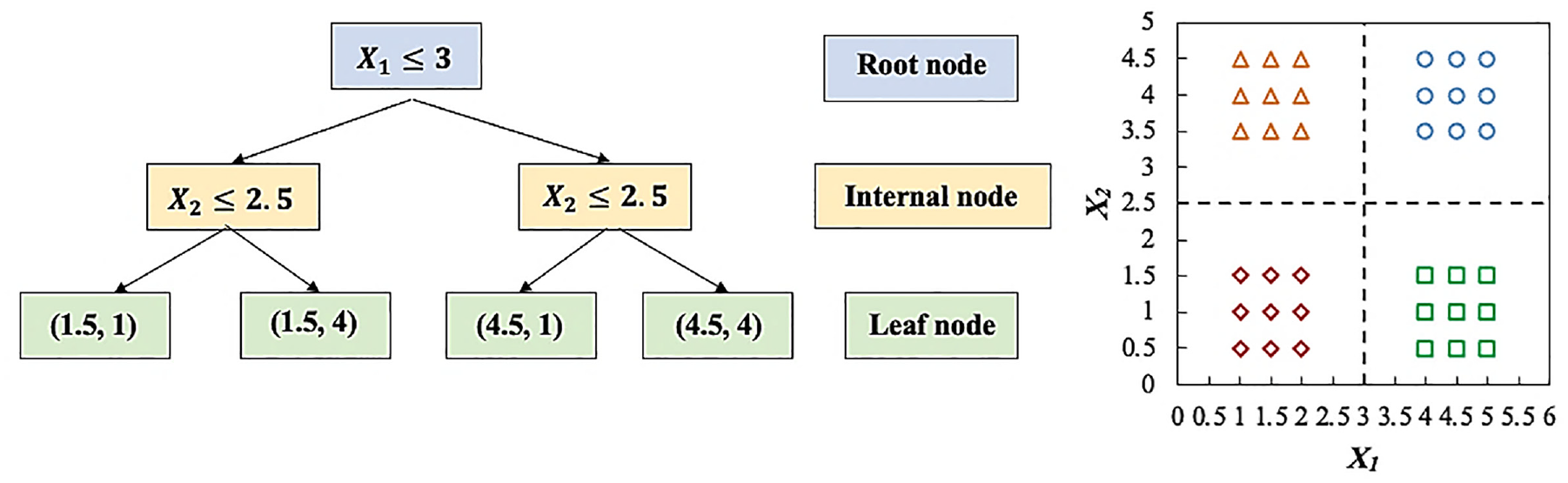
Decision tree structure.

Random Forest

RF is an ML ensemble method developed by Breiman ( 17 ). It aims to mitigate the limitations of individual decision trees by building a certain number of them in parallel and introducing randomness to each weak tree. RF generally does so by two processes: bootstrap aggregation and random feature selection. Take Figure 2 as a simplified example. The original dataset contains six entries of training examples from id₀ to id₅. Each training example has four features (x₀ to x₄) and one continuous output y. First, the RF algorithm creates N (N = 3 in this example) number of bootstrap datasets of the same size or smaller than the original dataset by randomly selecting training examples from the original dataset. Sampling with replacement ensures each bootstrap dataset is independent of its peers, as it does not depend on previously chosen samples. Moreover, each bootstrap dataset is made with randomly selected features, as in the case of our example, the first bootstrap dataset comprises two (x_o, x₁) randomly selected features out of four. This random feature selection helps to reduce correlation between individual trees by reducing variance and tackles the overfitting problem that plagues individual decision tree model. Finally, each N number of bootstrap dataset is used to create N numbers of individual decision trees as explained. It ensures that the individual trees are as independently as possible. In this way, the RF model is trained. While predicting with testing data samples, each input feature value is passed through its corresponding trees, and the independent output generated by each individual tree is averaged to get the final output from the RF model. It is noteworthy that the number of maximum features to randomly select while bootstrapping is one of the many crucial hyperparameters of the RF model. The other hyperparameter being the number of trees to build. Moreover, each individual tree has its own hyperparameters. These hyperparameters are optimized for a given predictive modeling problem to obtain an optimum RF model.

Figure 2.

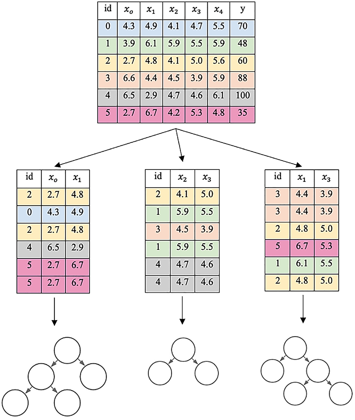
Random forest structure.

Gradient Boosted Tree

GBT is another ML ensemble technique where a sequence of weak decision trees is constructed in an iterative fashion. It was proposed by Friedman ( 18 ). The algorithm can be simplified as follows. Given the input training data ${(x_{i}, y_{i})}_{i = 1}^{n}$ and a predefined differential loss function $L (y_{i}, F (x))$ :

1. Initialize a base model with a constant value:

F_{0} (x) = \arg mi n_{γ} \sum_{i = 1}^{n} L (y_{i}, γ)

(1)

where $y_{i}$ is the observed value and $γ$ represents the predicted value that minimizes the loss function $\sum_{i = 1}^{n} L (y_{i}, γ)$ .

2. For m = 1 to M:

i. Compute pseudo-residuals:

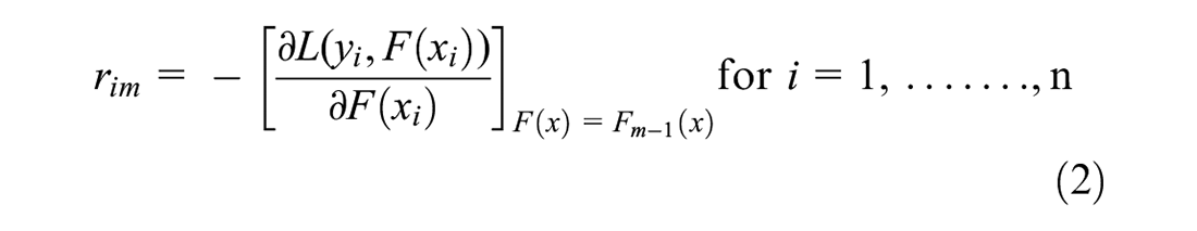
r_{im} = - {[\frac{\partial L (y_{i}, F (x_{i}))}{\partial F (x_{i})}]}_{F (x) = F_{m - 1} (x)} for i = 1, \dots \dots ., n

(2)

where $F (x_{i})$ is the previous model and M is the total number of trees.

ii. Fit a new regression tree to the $r_{im}$ residuals and divide the input feature space into terminal regions $R_{jm}$ for j = 1,….., $J_{m}$ . Here, $J_{m}$ represents the number of leaf nodes.

iii. For j = 1,…., $J_{m}$ compute:

γ_{jm} = \arg mi n_{γ} \sum_{x_{i} \in R_{ij}} L (y_{i}, F_{m - 1} (x_{i}) + γ)

(3)

iv. Update $F_{m} (x) = F_{m - 1} (x) + η \sum_{j = 1}^{J_{m}} γ_{m} I (x \in R_{jm})$

where $η$ represents learning rate and $\sum_{j = 1}^{J_{m}} γ_{m} I (x \in R_{jm})$ is the currently added tree.

3. Output $F_{M} (x)$

In sum, GBT optimizes a loss function by fitting a series of decision trees, where each successive tree tries to correct the errors of the previous ones. The algorithm starts with a base model, which is often a simple decision tree. Then it evaluates the performance of the model on the training data and calculates the gradient of the loss function with respect to the predictions made by the model. This gradient indicates the direction in which the model’s predictions can be improved to better fit the training data. The next tree is trained to predict the residual errors of the previous model. This process is repeated iteratively, with each new tree trained to predict the residual errors of the previous model, until a stopping criterion is met, such as a maximum number of trees (M). The final model, $F_{M} (x)$ , is the sum of all the decision trees, with each tree weighted by a learning rate ( $η$ ). The learning rate controls the contribution of each tree to the final prediction and helps to prevent overfitting by shrinking the contribution of each tree. Notably, learning rate and number of trees are two of the significant hyperparameters of a GBT model, which will be fine-tuned later in the model development process. Moreover, each decision tree has its own hyperparameters, as described earlier.

Methodology of ML Model Development

The development of any ML model has several general steps such as database compilation, model inputs selection, data division, training, hyperparameter optimization, and testing. An open-source ML library for the Python programming language called scikit-learn or sklearn ( 19 ) is used in this study to simulate the three tree-based models.

Database Compilation

A database of 80 pile load tests of square precast prestressed concrete (PPC) piles of varying widths and lengths that were collected from 34 project sites in Louisiana was used in this study to develop the ML models. Figure 3a illustrates the locations of these sites. The lengths of the piles range from 35 ft to 163 ft (11 m to 50 m), while the widths range from 14 in. to 30 in. (356 mm to 762 mm). The piles were subjected to a quick load test at about 14 days of driving, following the ASTM D1143 ( 20 ) procedure. The load–settlement curve for each pile load test, as shown in Figure 3b, was interpreted to determine the measured ultimate pile capacity using the Davisson’s offset limit method ( 21 ). This method defines the ultimate pile capacity as the load that causes the pile top to deflect by an amount equal to the calculated elastic compression plus 0.15 in. plus 1/120 of the pile’s width (B). The associated CPT tests were conducted close to each test pile. As the developed excess pore water pressure behind the cone base (u₂) can affect the overall stress measured by the cone tip, the cone tip resistance (q_c) readings for each CPT were corrected, q_t ( 22 , 23 ) for use in the ML models.

Figure 3.

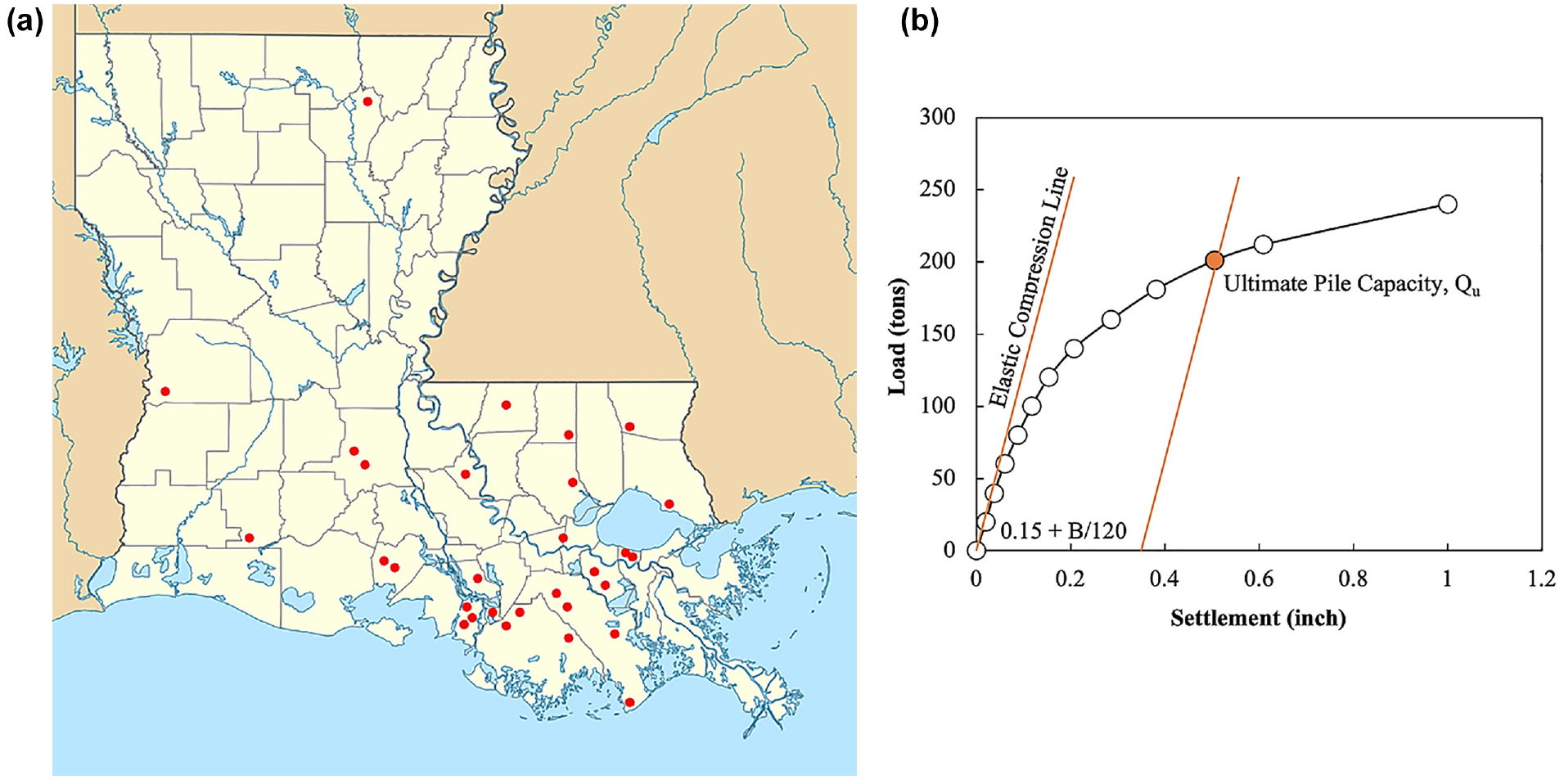
(a) Map of Louisiana indicating pile load test sites and (b) Davisson’s failure criterion.

Model Input and Output Parameters

The quality of ML predictions is highly dependent on the proper selection of input variables that influence the output, predicted ultimate pile capacity (Q_p). The well-known parameters that influence capacity are pile characteristics such as pile material, geometry, tip condition, installation type, load test process; and soil characteristics such as physical and mechanical properties, and so forth. However, since all the tested piles in the compiled database are square precast prestressed concrete driven piles with closed tips, many of these factors can be disregarded. In this study, the embedded length of pile (L_e) and pile width (B) along with the corresponding CPT data profile (corrected tip resistance, q_t, and sleeve friction, f_s) that reliably quantify the soil characteristics are considered as input variables. In addition, the variation of soil properties along the pile shaft, the embedded length of the pile, was considered and sub-divided into five equal segments as described in prior research ( 24 – 26 ). The averages of corrected cone tip resistance (q_t,avg) and sleeve friction (f_s,avg) along each of the five segments are determined independently. The failure influence zone is considered to range from 4B (B = pile width) above to 4B below pile tip, in which the average corrected tip resistance (q_t-tip) is determined separately. Consequently, 14 input variables are selected to develop the ML model, as shown in Figure 4.

Figure 4.

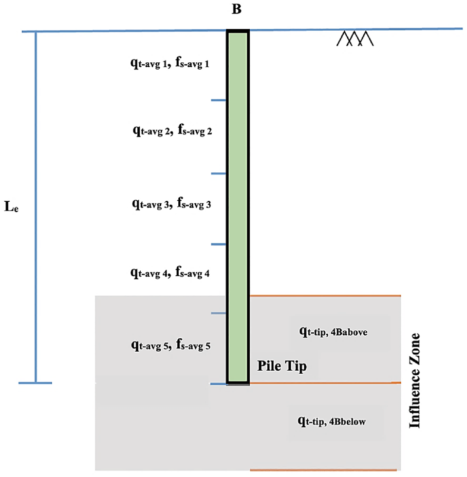
Input of the models.

Data Division

Before the start of training, the database is randomly divided into 80% for training and 20% for testing. The training subset is used to train the ML models, while the testing subset is utilized to evaluate the accuracy and generalization ability of the trained models. This division is carried out randomly through trial and error until the statistical properties (mean, standard deviation, range) of both subsets are approximately as close to each other as possible with minimum and maximum values included in the training subset ( 27 ).

Design and Training of Tree-Based ML Models

After data division, each of the three ML models (DT, RF, and GBT) is trained and assessed independently with the objective of identifying the model that provides the optimum or near optimum performance for the given task. Each model possesses some external tunable parameters called hyperparameters. These parameters regulate the learning process and must be set before the training process begins. Table 1 illustrates all the significant hyperparameters of the decision tree, RF, and GBT models tuned in this study, as denoted in scikit-learn ( 19 ).

Table 1.

Hyperparameters of Tree-Based Models

Hyperparameters	Variable type	Range	Applicable models
learning_rate	Continuous	0–∞	GBT
n_estimators	Discrete	1–∞	RF, GBT
max_features	Continuous	0–1	RF, GBT
max_depth	Discrete	1–∞	DT, RF, GBT
min_samples_split	Discrete	2–∞	DT, RF, GBT
min_samples_leaf	Discrete	1–∞	DT, RF, GBT

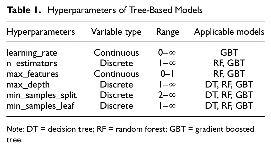
Note: DT = decision tree; RF = random forest; GBT = gradient boosted tree.

Since both the RF and GBT models are built with decision trees as base learners, they have some common hyperparameters (max_depth, min_samples_split, min_samples_leaf) with decision tree models. Apart from these, RF and GBT have two crucial hyperparameters to be tuned: the number of decision trees to be combined, denoted as n_estimators; and the number of random features to consider while building trees, denoted as max_features. The GBT model has an additional hyperparameter called learning_rate. It is noteworthy that the three tree-based models have numerous hyperparameters. Only the main hyperparameters that significantly affect the performance of ML models based on literature are explored in this study ( 28 ).

It is necessary to evaluate multiple combinations of hyperparameter settings since one set may perform well in one case but poorly in another case. The process of determining the optimal combination of hyperparameter settings for a certain problem is known as hyperparameter optimization. In previous studies using ML to predict pile capacity ( 6 – 12 ), the produced models were optimized manually through a trial and error procedure that is tedious and computationally expensive. In this work, a more effective method termed random search is employed for hyperparameter optimization. The random search procedure begins by specifying a finite number of possible values for each hyperparameter, creating a hyperparameter search space. The search algorithm then selects random combinations of hyperparameters from the search space. Each hyperparameter combination represents a distinct candidate model. The performance of each candidate model is then determined using a k-fold cross-validation procedure.

In the k-fold cross-validation procedure, as depicted in Figure 5, the training data is first randomly split into k-folds (subsets). Then, the candidate model undergoes an iterative evaluation procedure. During each evaluative iteration, k-1 of the folds is used to train the candidate model, while the remaining fold is utilized to evaluate the model’s performance. This procedure is repeated until each fold has been used exactly once as a validation set, resulting in k training and validation iterations for each candidate model. Finally, the average of a performance metric from each iteration is used to estimate the overall performance of the candidate model. This process guarantees that a model undergoing this process generalizes well to all training data segments.

Figure 5.

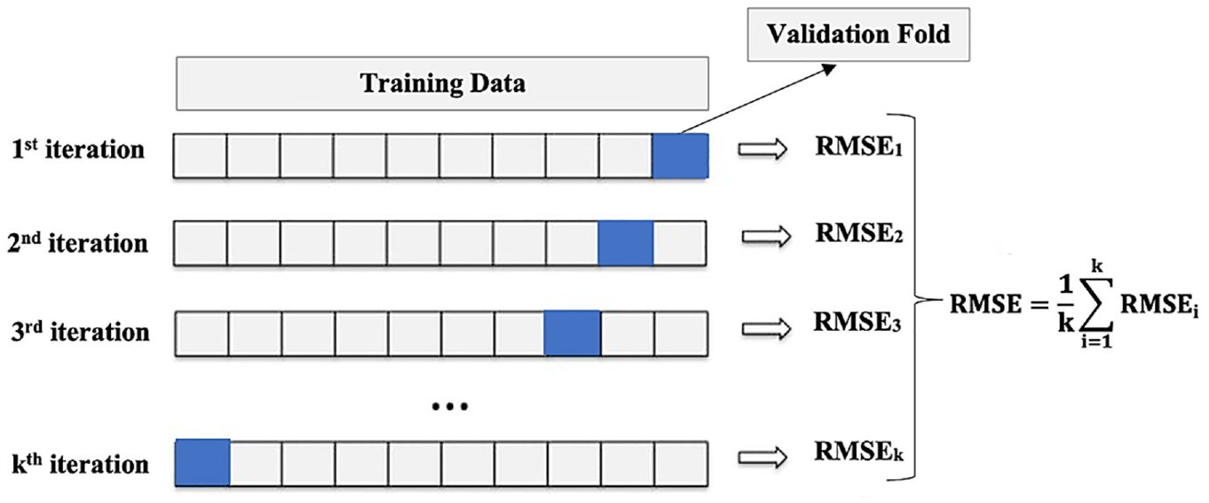
k-fold cross-validation.

In this study, each tree-based model (DT, RF, and GBT) was independently subjected to this random search procedure to identify three optimal models. For each of the three techniques, the search space was set by examining numerous ranges of hyperparameter values, and hundreds of candidate models were evaluated using 10-fold cross-validation until the optimal models were identified. As the training dataset is rather small, 10-fold cross-validation is utilized. In particular, the optimization begins with a broad search space as the viable hyperparameter domain chosen by manual testing or domain expertise. The search space is then reduced based on the regions of well-performing hyperparameter values currently investigated, or a new search space is searched if necessary. The optimal hyperparameter settings found for each model are depicted in Table 2. The selected optimal model is then trained one last time on the entire training set before being used to evaluate the train and test subsets.

Table 2.

Combination of Hyperparameters of Optimum Tree-Based Models

Hyperparameters	Optimum tree-based model
Hyperparameters	Decision tree	Random forest	Gradient boosted tree
learning_rate	na	na	0.02
n_estimators	na	210	185
max_features	na	0.75	0.5
max_depth	5	8	3
min_samples_split	11	2	4
min_samples_leaf	3	1	1

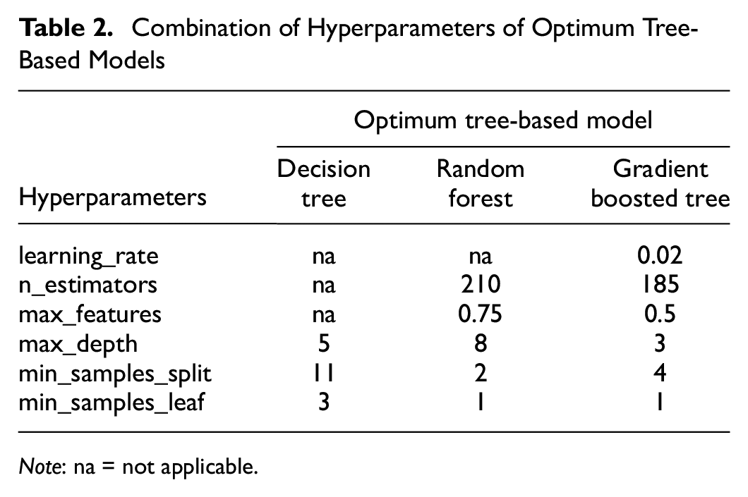
Note: na = not applicable.

Testing Results of Tree-Based ML Models

After locating the optimal models by random search, a final evaluation is performed on the 20% test subset to ensure that these models can be robustly generalized. For a model to be adequately generalized, it must not overfit the training data and have minimal bias and variance. In particular, it should produce low error rates on both the training and testing data. The entire random search process is repeated using a different search space to find the optimal model architecture until satisfactory results are obtained in this final evaluation on the test subset. The coefficient of determination (R²) and root mean squared error (RMSE) are statistical measures usually used to evaluate the accuracy and generalizability of these models. The R² and RMSE are computed using the following equations:

R^{2} = 1 - \frac{\sum_{i = 1}^{n} {(Q_{mi} - Q_{pi})}^{2}}{\sum_{i = 1}^{n} {(Q_{mi} - {\bar{Q}}_{m})}^{2}}

(4)

RMSE = \sqrt[2]{\frac{1}{n} \sum_{i = 1}^{n} {(Q_{pi} - Q_{mi})}^{2}}

(5)

where ${\bar{Q}}_{m} = \frac{1}{n} \sum_{i = 1}^{n} Q_{mi}$ , $Q_{p}$ = predicted pile capacity, $Q_{m}$ = measured pile capacity, and n = number of observations.

Table 3 presents the R² and RMSE of predicted versus measured ultimate pile capacity based on the training and testing phases of optimum decision tree, RF and GBT models. Figure 6 graphically depicts the comparison between the measured and predicted ultimate pile capacity for the three ML models. The results of an ANN model that was developed in a previous study ( 26 ) is also added to Table 3 for comparison. This ANN model was developed using the same 80 pile load test database and the same 14 input parameters to predict the ultimate pile capacity. This provides an insight performance comparison between the tree-based models and the ANN model.

Table 3.

Results of the Optimum Models on Training and Testing Phase

Tree-based machine learning models	Phase	Coefficient of determination, R²	Root mean squared error (tons)
Decision tree	Training	0.91	51.6
Decision tree	Testing	0.66	99.96
Random forest	Training	0.98	25.78
Random forest	Testing	0.94	43.23
Gradient boosted tree	Training	0.99	16.9
Gradient boosted tree	Testing	0.97	27.2
Artificial neural network ( 26 )	Training	0.99	10.18
Artificial neural network ( 26 )	Testing	0.97	24.9

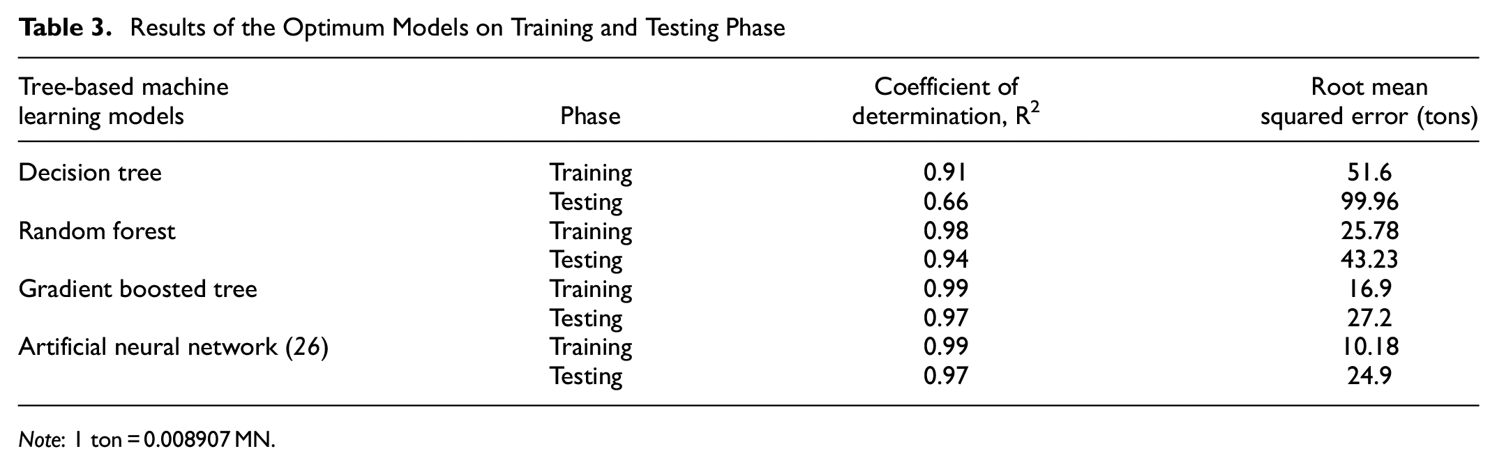
Note: 1 ton = 0.008907 MN.

Figure 6.

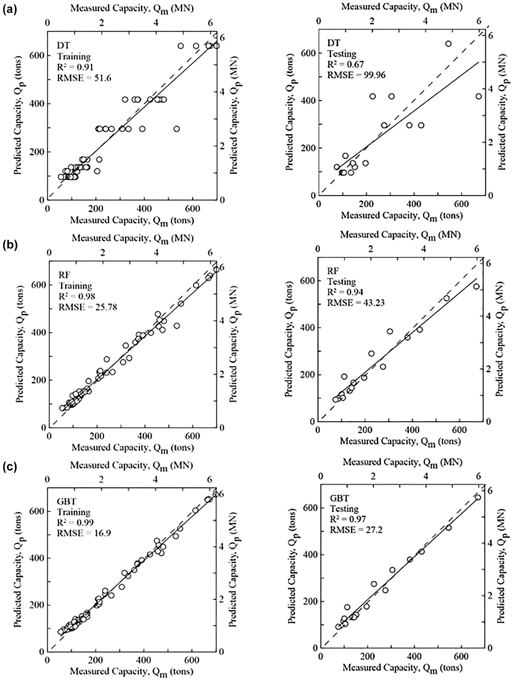
Measured versus predicted pile capacity for: (a) decision tree, (b) random forest, and (c) gradient boosted tree models based on training (left) and testing (right) subsets.

It can be observed that the DT model has the worst performance compared with the other models in both training and testing phases. Intelligibly, the testing RMSE (= 99.96 tons) is significantly higher than the training RMSE (= 51.6 tons) for the decision tree model, which indicates high overfitting. The second-best model in this comparison is RF, which has a testing R² = 0.94 and RMSE = 43.23tons. Noticeably, the overfitting condition gets much better when the RF model is used compared with the DT model. However, the GBT model outperforms both the DT and RF models and demonstrates comparatively the best performance and generalization ability in this study. The R² value for the GBT model is the same as the ANN model in both training (R² = 0.99) and testing (R² = 0.97) phases. Although the RMSE values are slightly lower in the ANN than GBT in both phases, the GBT model gives a competitive performance in predicting the ultimate pile capacity from CPT data.

Comparison with Selected Pile-CPT Methods

In a previous study, Amirmojahedi and Abu-Farsakh ( 13 ) conducted a comprehensive evaluation of 18 direct pile-CPT methods for estimating the ultimate pile capacity using a database of pile load tests from Louisiana. Their study demonstrated that the LCPC (Laboratoire Central des Ponts et Chaussées) ( 1 ), ERTC3 (European Regional Technical Committee 3) ( 3 ), probabilistic ( 4 ), and UF (University of Florida) ( 2 ) methods are the four top-performing direct pile-CPT methods for accurate estimation of ultimate pile capacity based on multiple statistical criteria. Using the same 20% test subset, the top-performing GBT model produced in this study is compared against the four top-performing pile-CPT methods from a previous study ( 13 ) using the following three statistical criteria:

The slope of the best-fit line (Q_fit/Q_m) of predicted (Q_p) versus measured (Q_m) ultimate pile capacity found through performing linear regression without intercept term and the RMSE and R² calculated via Equations 4 and 5.

The arithmetic mean (μ) and coefficient of variation (COV) of Q_p/Q_m.

The 20% accuracy level derived from the log-normal distribution of Q_p/Q_m.

Based on these three criteria, the rank index (RI) proposed by Abu-Farsakh and Titi ( 29 ) is calculated for each method, which quantifies the performance and ranks the different methods according to the formula RI = R₁ + R₂ + R₃. Here R₁, R₂, and R₃ are the criteria for ranking. The smaller the RI value, the better is the method’s performance. The final ranking of all reported methods in this study is shown in Table 4.

Table 4.

Comparison of Tree-Based ML Models with Selected Pile-CPT Methods

Method	First criterion				Second criterion			Third criterion		Ranking
Method	Q_fit/Q_m	R²	RMSE (tons)	R₁	μ	COV	R₂	Log normal (%)	R₃	RI	Final rank
GBT	0.98	0.97	27.20	1	1.07	0.17	2	84.8	1	4	1
UF	1.04	0.87	67.31	2	1.05	0.24	1	74.3	3	6	2
Probabilistic	1.06	0.88	68.01	3	1.06	0.23	3	75.1	2	8	3
LCPC	1.13	0.82	97.53	4	1.11	0.28	5	61.7	4	13	4
ERTC3	1.09	0.77	104.10	5	1.10	0.32	4	59.5	5	14	5

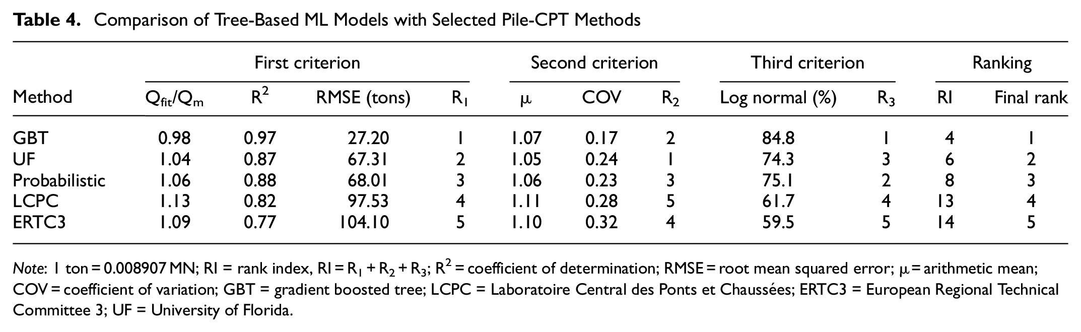
Note: 1 ton = 0.008907 MN; RI = rank index, RI = R₁ + R₂ + R₃; R² = coefficient of determination; RMSE = root mean squared error; μ = arithmetic mean; COV = coefficient of variation; GBT = gradient boosted tree; LCPC = Laboratoire Central des Ponts et Chaussées; ERTC3 = European Regional Technical Committee 3; UF = University of Florida.

The first criterion R₁ is found by conducting a linear regression between the measured (Q_m) and predicted (Q_p) ultimate pile capacity values of the test subset and calculating the slope (Q_fit/Q_m) of the best-fit line. The results of Q_m versus Q_p plots for GBT, UF, probabilistic, LCPC, and ERTC3, are presented in Figure 7, a to e , respectively. It can be observed from Table 4 and Figure 7 that, for the first criterion, the GBT model has the best performance with Q_fit/Q_m = 0.98, R² = 0.97, and RMSE = 27.20 tons. Since Q_fit = 0.98 Q_m, this model tends to underestimate the measured ultimate capacity, on average by 1%. It can also be seen that the four pile-CPT methods tend to overpredict the measured ultimate capacity. For example, the UF method tends to overpredict by an average of 4% with better RMSE (= 67.31 tons) as compared with the other pile-CPT methods and is ranked second according to the first criterion.

Figure 7.

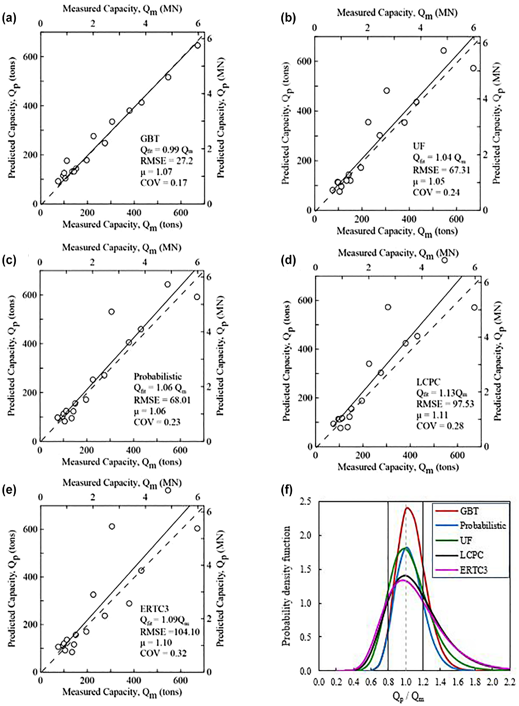
Performance of gradient boosted tree (GBT) model compared with four direct pile-CPT methods: (a) GBT, (b) University of Florida (UF), (c) probabilistic, (d) Laboratoire Central des Ponts et Chaussées (LCPC), (e) European Regional Technical Committee 3 (ERTC3), and (f) log-normal distribution of predicted versus measured pile capacity, Q_p/Q_m.

The second criterion R₂ is based on the arithmetic mean (μ) and coefficient of variance (COV) of the Q_p/Q_m values of the testing subset. By evaluating μ and COV, one can determine the accuracy and precision of a procedure on a fundamental level. The methods with μ > 1 overestimate the measured pile capacity, whereas those with μ < 1 underestimate it. The COV is the ratio of standard deviation to mean, which reveals the level of variation around the mean. In short, values of μ closer to one and COV values closer to zero are deemed superior. The values of μ and COV and the corresponding ranking based on this criterion (R₂) is shown on Table 4. The UF method ranked first based on the R₂ criterion with μ value (= 1.05) closest to one. The GBT model ranked second with μ = 1.07, but it has the lowest COV value (= 0.17) as compared with other methods.

The third criterion R₃ is determined by the log-normal distribution of Q_p/Q_m. The theoretical range of the ratio Q_p/Q_m is between zero and infinity, with an optimum value of one. Consequently, the distribution of Q_p/Q_m is asymmetrical, and underprediction and overprediction do not receive equal weight. According to Briaud and Tucker ( 30 ), the log-normal distribution captures the characteristics of Q_p/Q_m much better than the normal distribution. The log-normal density function is given as follows:

f (x) = \frac{1}{\sqrt{2 π} σ_{\ln} x} e^{[\frac{- 1}{2} {(\frac{\ln (x) - μ_{\ln}}{σ_{\ln}})}^{2}]}

(6)

where x = Q_p/Q_m, $σ_{\ln}$ = standard deviation of ln(Q_p/Q_m), and $μ_{\ln}$ = mean of ln(Q_p/Q_m).

Using Equation 6, the log-normal distribution of the ratio Q_p/Q_m of the test subset for each method is created as shown in Figure 7f. It depicts the comparison of log-normal distributions for the methods. The probability corresponding to $\pm 20 %$ accuracy is the likelihood that the predicted pile capacity will be within $0.8 Q_{m} \leq Q_{p} \leq 1.2 Q_{m}$ . It is obtained by computing the area under the log-normal distributions within this specified range. Higher probability value means better performance of the method. Table 4 displays the probabilities associated for each method. The GBT model has the highest probability value of 84.8%, and is ranked top, followed by the UF, probabilistic, and LCPC. Based on this criterion, ERTC3 ranks the last with a 59.5% probability.

Finally, the GBT model and the four pile-CPT methods are given overall ranks based on the three statistical criteria via RI. As shown in Table 4, the GBT is ranked first with the lowest RI = R₁ + R₂ + R₃ = 1 + 2 + 1 = 4. Among the pile-CPT methods, the UF and probabilistic show almost similar performance based on all three criteria and ranked 2 and 3 accordingly. However, the LCPC and ERTC3 have the lowest performance in all criteria.

Discussion

The results of this study indicate that the GBT model performed better than the other explored methods. Thus, it is suggested to be a “better alternative” to direct pile-CPT methods that are meant to complement the common static analyses (total stress and effective stress methods). However, currently the use of such ML models in pile-design is at early stages in practice. Thus, to foster confidence in ML based pile-design among designers, ML models should be used in conjunction with other design methods (i.e., direct pile-CPT methods, static analyses) and pile load tests. For example, if CPT tests and pile load test(s) are conducted for a certain site, a comparison can be done among the predicted capacities from ML models, the direct pile-CPT methods and the measured capacities from available pile load test(s). If the measured and predicted values are different, a correction should be developed to account for the difference between the measured capacities and predicted capacities from ML for the specific site. This correction can be applied to the design of other piles for same site, thus reducing the number of pile load tests needed for the project. This practice will gradually reduce the dependency on static analysis methods and increase confidence in and dependency on ML based pile-design. Thus, for now the use of such ML models should be limited to preliminary estimation or validation purposes in pile design. However, there are some general recommendations to keep in mind while implementing ML models in practice:

Since the database used to train the ML models exclusively contained only precast prestressed concrete (PPC) driven piles, it is not recommended to use the model for other pile types without verification.

Since all 80 pile load tests are situated in Louisiana, the models should perform well for clayey Louisiana soils, and other locations with similar geotechnical characteristics.

The inputs of CPT data and pile properties should be approximately within the following range as utilized in model training:

○ 35 ft (11 m) ≤ Embedded pile length (L_e) ≤ 163 ft (50 m)

○ 14 in. (356 mm) ≤ Pile width (B) ≤ 30 in. (762 mm)

○ 1.59 tsf (ton per square foot) (0.15 MPa) ≤ Corrected cone tip resistance (q_t) ≤ 327 tsf (31.39 MPa)

○ 0.01 tsf (0.00096 MPa) ≤ Sleeve friction (f_s) ≤ 3.35 tsf (0.32 MPa)

The output of the ML models, ultimate pile capacity in the training data is within the range of 55 tons (0.49 MN) to 699 tons (6.22 MN). Therefore, the model should work better in predicting the pile capacities within this range.

Summary and Conclusion

This study investigated three variants (DT, RF, GBT) of tree-based ML models to accurately predict the ultimate capacity of single driven PPC piles from CPT data. A local database of static pile load tests and the accompanying CPT test results was compiled for the development of these models. The measured ultimate load capacity (Q_m) was determined using the Davisson’s interpretation method from the load–settlement curve from each pile load test. A total of 14 input pile and soil parameters were selected to predict ultimate pile capacity. Using the same test data, the performance of the best tree-based model (GBT) was compared with the best-performing direct pile-CPT methods from a previous study ( 13 , 14 ): the UF, probabilistic, ERTC3, and LCPC methods. Finally, the performance of GBT and pile-CPT methods were evaluated and ranked using multiple statistical criteria. Based on the findings of this study, the following conclusions can be made:

ML techniques can be trained and used to predict the ultimate capacity of piles from CPT data effectively and accurately.

Among the three simulated tree-based ML models (DT, RF, GBT) developed in this study, the GBT algorithm was demonstrated to be the best-performing ML model in estimating the ultimate capacity of piles from CPT data for both the training (R² = 0.99, RMSE = 16.9 tons) and testing (R² = 0.97, RMSE = 27.2 tons) subsets. The decision tree and RF models somehow tend to overfit the training data. The RF model performed better than the decision tree model, with testing R² = 0.94 and RMSE = 43.23 tons.

The results showed that the GBT model performed comparably with an ANN model that was developed in a previous study using the same dataset and input parameters. Thus, it is evident that the GBT model can be successfully utilized to estimate the ultimate pile capacity from CPT data with good accuracy.

Using the same test data, the comparison between the GBT model and the four top-performing direct pile-CPT methods (based on previous study) revealed that the GBT model outranked those methods in estimating the ultimate pile capacity from CPT data. Nevertheless, typical approaches like UF and probabilistic pile-CPT methods yielded quite similar results whereas the LCPC and ERTC3 showed the worst performance.

As black-box ML models, the tree-based algorithms cannot provide hand-calculable equations for use in pile design. However, the high prediction accuracy and generalization performance of those models as compared with pile-CPT methods significantly outweigh this lack of interpretability. Notably the ML models also provide more accurate predictions when applied within ranges of each input variable of the training data. Therefore, the GBT model should perform better for square PPC piles driven on a subsurface with approximately similar CPT profiles to those that were presented to the model during training.

Footnotes

Acknowledgements

The authors would like to express gratitude to Louisiana Department of Transportation and Development engineers for their continuous support and help throughout the study.

Authors Contributions

The authors confirm contribution to the paper as follows: study conception and design: M. Shoaib, M. Abu-Farsakh; data collection: M. Shoaib, M. Abu-Farsakh; analysis and interpretation of results: M. Shoaib, M. Abu-Farsakh; draft manuscript preparation: M. Shoaib, M. Abu-Farsakh. All authors reviewed the results and approved the final version of the manuscript.

Declaration of Conflicting Interests

The author(s) declared no potential conflicts of interest with respect to the research, authorship, and/or publication of this article.

Funding

The author(s) disclosed receipt of the following financial support for the research, authorship, and/or publication of this article: This research project is funded by the Louisiana Transportation Research Center (LTRC Project No. 17-2GT) and the Louisiana Department of Transportation and Development (State Project No. DOTLT1000165).

ORCID iD

Murad Y. Abu-Farsakh

References

Bustamante

Gianeselli

Pile Bearing Capacity Prediction by Means of Static Penetrometer CPT. Proc., 2nd European Symposium on Penetration Testing, Amsterdam, The Netherlands, 1982, pp. 493–500.

Bloomquist

McVay

M. C.

Updating Florida Department of Transportation’s (FDOT) Pile/Shaft Design Procedures Based on CPT & DTP Data. UF Project 00005780. University of Florida, Gainesville, 2007.

McVay

Bloomquist

Horhota

Lai

New Ultimate Pile Capacity Prediction Method Based on Cone Penetration Test (CPT). Canadian Geotechnical Journal, Vol. 49, No. 8, 2012, pp. 961–967.

Abu-Farsakh

M. Y.

Titi

H. H.

Probabilistic CPT Method for Estimating the Ultimate Capacity of Friction Piles. Geotechnical Testing Journal, Vol. 30, No. 5, 2007, pp. 387–398.

De Cock

Legrand

Design of Axially Loaded Piles - European Practice. Proc., ERTC-3 Seminar, Brussels, CRC Press, London, 1997.

Shahin

M. A.

Intelligent Computing for Modeling Axial Capacity of Pile Foundations. Canadian Geotechnical Journal, Vol. 47, No. 2, 2010, pp. 230–243.

Kordjazi

Pooya Nejad

Jaksa

M. B.

Prediction of Ultimate Axial Load-Carrying Capacity of Piles Using a Support Vector Machine Based on CPT Data. Computers and Geotechnics, Vol. 55, 2014, pp. 91–102.

Alkroosh

Nikraz

Correlation of Pile Axial Capacity and CPT Data Using Gene Expression Programming. Geotechnical and Geological Engineering, Vol. 29, 2011, pp. 725–748.

Ghorbani

Sadrossadat

Bolouri Bazaz

Rahimzadeh Oskooei

Numerical ANFIS-Based Formulation for Prediction of the Ultimate Axial Load Bearing Capacity of Piles Through CPT Data. Geotechnical and Geological Engineering, Vol. 36, 2018, pp. 2057–2076.

10.

Harandizadeh

Jahed Armaghani

Khari

A New Development of ANFIS-GMDH Optimized by PSO to Predict Pile Bearing Capacity Based on Experimental Datasets. Engineering with Computers, Vol. 37, 2021, pp. 685–700.

11.

Ardalan

Eslami

Nariman-Zadeh

Piles Shaft Capacity from CPT and CPTu Data by Polynomial Neural Networks and Genetic Algorithms. Computers and Geotechnics, Vol. 36, 2009, pp. 616–625.

12.

Baziar

M. H.

Kashkooli

Saeedi-Azizkandi

Prediction of Pile Shaft Resistance Using Cone Penetration Tests (CPTs). Computers and Geotechnics, Vol. 45, 2012, pp. 74–82.

13.

Amirmojahedi

Abu-Farsakh

Evaluation of 18 Direct CPT Methods for Estimating the Ultimate Pile Capacity of Driven Piles. Transportation Research Record: Journal of the Transportation Research Board, 2019. 2673: 127–141.

14.

Amirmojahedi

Estimation of the Axial and Lateral Capacity of Driven Piles from the Results of Cone Penetration Test and Finite Element Analysis. PhD dissertation. Louisiana State University, Baton Rouge, 2020.

15.

Breiman

Friedman

Olshen

Stone

Classification and Regression Trees. Wadsworth, Belmont, CA, 1984.

16.

Gareth

Daniela

Trevor

Robert

An Introduction to Statistical Learning with Applications in R. Springer, New York, NY, 2013.

17.

Breiman

Random Forests. Machine Learning, Vol. 45, 2001, pp. 5–32.

18.

Friedman

J. H.

Stochastic Gradient Boosting. Computational Statistics & Data Analysis, Vol. 38, No. 4, 2002, pp. 367–378.

19.

Pedregosa

Varoquaux

Gramfort

Michel

Thirion

Grisel

Blondel

, et al. Scikit-Learn: Machine Learning in Python. Journal of Machine Learning Research, Vol. 12, 2011, pp. 2825–2830.

20.

ASTM International. Standard Test Method for Deep Foundations Under Static Axial Compressive Load. ASTM International, West Conshohocken, PA, 2013.

21.

Davisson

High Capacity Piles. Soil Mechanics Lecture Series on Innovation in Foundation Construction, ASCE, Illinois Section, Chicago, 1972, pp. 81–112.

22.

Campanella

R. G.

Gillespie

D. G.

Robertson

P. K.

Pore Pressures During Cone Penetration Testing. Department of Civil Engineering, University of British Columbia, Canada, 1981.

23.

Lunne

Eidsmoen

Gillespie

Howland

J. D.

Laboratory and Field Evaluation of Cone Penetrometers. Paper Presented at the Use of In Situ Tests in Geotechnical Engineering conference, Blacksburg, VA, 1986.

24.

Pooya Nejad

Jaksa

M. B.

Kakhi

McCabe

B. A.

Prediction of Pile Settlement Using Artificial Neural Networks Based on Standard Penetration Test Data. Computers and Geotechnics, Vol. 36, No. 7, 2009, pp. 1125–1133.

25.

Pooya Nejad

Jaksa

M. B.

Load-Settlement Behavior Modeling of Single Piles Using Artificial Neural Networks and CPT Data. Computers and Geotechnics, Vol. 89, 2017, pp. 9–21.

26.

Mojumder

M. A. H.

Evaluation of Undrained Shear Strength of Soil, Ultimate Pile Capacity and Pile Set-Up Parameter from Cone Penetration Test (CPT) Using Artificial Neural Network (ANN). Master’s thesis. Louisiana State University, Baton Rouge, 2020.

27.

Shahin

M. A.

Maier

H. R.

Jaksa

M. B.

Data Division for Developing Neural Networks Applied to Geotechnical Engineering. Journal of Computing in Civil Engineering, Vol. 18, No. 2, 2004, pp. 105–114.

28.

Yang

Shami

On Hyperparameter Optimization of Machine Learning Algorithms: Theory and Practice. Neurocomputing, Vol. 415, 2020, pp. 295–316.

29.

Abu-Farsakh

M. Y.

Titi

H. H.

Assessment of Direct Cone Penetration Test Methods for Predicting the Ultimate Capacity of Friction Driven Piles. Journal of Geotechnical and Geoenvironmental Engineering, Vol. 130, No. 9, 2004, pp. 935–944.

30.

Briaud

J. L.

Tucker

L. M.

Measured and Predicted Axial Response of 98 Piles. Journal of Geotechnical Engineering, Vol. 114, No. 9, 1988, pp. 984–1001.

Exploring Tree-Based Machine Learning Models to Estimate the Ultimate Pile Capacity From Cone Penetration Test Data

Abstract

Keywords

Overview of Tree-Based Machine Learning

Decision Tree

Random Forest

Gradient Boosted Tree

Methodology of ML Model Development

Database Compilation

Model Input and Output Parameters

Data Division

Design and Training of Tree-Based ML Models

Testing Results of Tree-Based ML Models

Comparison with Selected Pile-CPT Methods

Discussion

Summary and Conclusion

Footnotes

Acknowledgements

Authors Contributions

Declaration of Conflicting Interests

Funding

ORCID iD

References