
Abstract
Path planning and trajectory tracking are very meaningful for the field of autonomous driving, but currently path planning still has problems such as non-optimal paths and insufficiently accurate paths. This paper addresses the issue of path planning by proposing a improved A-star algorithm and locally zooming on the map technique to achieve precise path planning. Compared with the conventional method, this method reduces the time by 23% and the path length by 21% in the scenarios shown in the paper, respectively, and provides a reference for related research. Moreover, trajectory tracking was achieved using the improved LQR control. Compared with the conventional method, the improved LQR control algorithm reduces the average error by 80% in the scenario shown in the paper. Firstly, the A-star algorithm is enhanced by incorporating an unknown path cost estimation function, thereby improving the effect of its path planning in complex environments. Additionally, the method of locally zooming on the map is incorporated, effectively enhancing the accuracy and safety of path planning. Building upon the path planning, further improvements are made to the LQR control algorithm, enabling autonomous deceleration in complex sections, which facilitates better trajectory tracking and enhances the motion control performance of the robot during practical operations.
Introduction
In recent years, thanks to the vigorous development of cloud computing and IoT technologies, the advancement of smart cities has become an increasingly prominent topic of interest in both academia and industry. The emergence of new technologies has provided us with fresh ideas and techniques for constructing more intelligent cities. As mobile robots become more prevalent in everyday life, figuring out a fast and efficient path for robots has become a popular research direction. In order for a mobile robot to efficiently finish its assigned tasks, it is essential to plan an optimal path. Path planning refers to the process in which a mobile robot, utilizing sensor information derived from its complex working environment, figures out a path from the starting point to the ending point while satisfying certain evaluation criteria. Additionally, the robot must safely and reliably navigate around all obstacles in the way during its movement. Depending upon the known level of environment, path planning can be classified into global path planning and local path planning. The main algorithms used today are Genetic Algorithms, Artificial Potential Field Algorithms, Free Space Methods, Artificial Neural Network Algorithms, Dijkstra’s Algorithm and A-star Algorithm. The A-star algorithm is extensively applied by virtue of its simple principle, ease of implementation, high efficiency, and capability to search for optimal solutions. 1
The A-star algorithm was proposed by Nilsson in 1980 based on the Dijkstra’s algorithm. It is a global path planning algorithm based on heuristic search. However, the A-star algorithm is not guaranteed to always find an optimal solution, especially if the heuristic function is not an appropriate choice. Also, the A-star algorithm is not complete, that is, it is not guaranteed to find a solution in finite time. Duchoň et al. used a skip-point search strategy to optimize the A-star algorithm. Despite a significant reduction in search time, the derived path tends to be longer and typically longer than other eight-connected algorithms. 2 Tang et al. proposed a geometry-based A-star algorithm that filters out nodes in the closed list using two functions, eliminating nodes that do not meet the requirements to avoid generating irregular paths. Nevertheless, the path is still not optimal, and besides, the article does not take into account the minimum traffic size of the robot. 3 Ju et al. proposed an optimized A-star algorithm inspired by the shortest line segment between two points. Although this method can be used to find shorter paths in some cases, it is faced with the same problem as the research of Ju et al., which is that it requires too much time and calculated quantity, making the algorithm less efficient. 4 The two-way optimization method proposed by Zhang et al. can be used to delete useless nodes, thus effectively shortening the length of the path, but the calculated quantity is too large, the time required is too long and the efficiency is low. 5 Chen et al. proposed an improved A-star algorithm to expand concave obstacles, thus reducing the number of nodes to be searched, but this will increase the area of obstacles, which may lead to longer planned paths that are not optimal. 6
From the above research, it can be learned that many scholars have made improvements to the A-star algorithm. However, the following problems have not been well addressed: the A-star algorithm combined with other algorithms deviate from the desired trajectory of the algorithm, resulting in non-optimal paths, and the calculated quantity is much higher than that of traditional A-star algorithms. Furthermore, most of the research on path planning is based on grid maps, where a large grid size can result in insufficient accuracy, while a small grid size can cause excessive calculated quantity. To address the aforementioned issues, an improved A-star algorithm is designed in this paper. It involves locally zooming the grid map while simultaneously shortening the length of the path planning.
The remaining parts of this paper are organized in the following way. Section 2 gives a brief introduction to the principles of path planning and the A-star algorithm. Section 3 presents the utilization of the improved A-star algorithm and the method of locally zooming the map for precise path planning. The simulation of path planning are described in Section 4. Section 5 incorporates the basic principles of LQR control as well as the improved approach. The simulation results of the improved LQR control are presented in Section 6. The conclusion is drawn in Section 7.
Path planning
Methods of path planning
Nowadays the application of AI methods has become more and more common in all kinds of industries, and the field of path planning is no exception.7–9 Path planning is a fundamental problem in computer science, aiming to find the shortest or optimal path from the starting point to the ending point, in a bid to satisfy specific requirements and constraints. Path planning is crucial in numerous applications, including autonomous driving, robot navigation, air traffic control, logistics, and transportation, among others. In path planning, the starting point and the ending point are regarded as nodes, while the roads between nodes are regarded as edges. The path planning algorithm is intended to find the shortest or optimal path from the starting point to the ending point by searching the graph. 10
The basic idea of path planning algorithms is to conduct a search in the graph to find the shortest or optimal path. The search process can be performed using breadth-first search, depth-first search, and typical algorithms such as Dijkstra’s algorithm and A-star algorithm.
Breadth-first search is a queue-based algorithm that starts the search from the starting point, adds its neighboring nodes to the queue, and marks them as “accessed.” Thereafter, the algorithm takes the next node in the queue as the current node and continues searching for the next node until the ending point is found. 11
Depth-first search is a stack-based algorithm that starts the search from the starting point and adds its neighboring nodes to the stack. Thereafter, the algorithm takes the top element of the stack as the current node and continues searching for the next node until the ending point is found. Unlike breadth-first search, depth-first search explores one branch first until it can no longer continue, then backtracks to the previous node and continues exploring another branch. 12
The Dijkstra’s algorithm is a shortest path algorithm based on the greedy strategy that starts the search from the starting point and calculates the shortest distance from each node to the starting point. In the course of search, the algorithm chooses the closest node to the starting point among the unmarked nodes and updates the distances of the nodes adjacent to it. This course is repeated until the ending point is found. 13
The A-star algorithm is an optimal path algorithm that combines the greedy strategy with a heuristic function. It chooses the next node by estimating the distance from each node to the ending point. This estimated value is called “heuristic function,” which can be designed as appropriate, for example, Euclidean distance or Manhattan distance. In the course of search, the A-star algorithm picks the following best node, considering the genuine length from the node to the starting point and the predicted length from the node to the endpoint. 14 Apart from graph-based search algorithms, there are also sampling-based path planning algorithms. 15 Wherein, the well-known sampling-based path planning algorithms cover the Rapidly-exploring Random Tree (RRT) algorithm and the Probabilistic Roadmap (PRM) algorithm.16,17 In addition to graph-based search algorithms and sampling-based algorithms, there are other path planning algorithms available, for example, the fast interpolation method, multi-objective optimization algorithm.
In practical applications, path planning must take into account various factors and constraints, for example, the maximum speed, maximum acceleration, minimum curvature radius of the vehicle, traffic flow, traffic lights, and the like. To address these issues, the path planning algorithms must integrate a variety of techniques, for example, dynamic programing, optimization methods, machine learning, and more. Moreover, modern path planning algorithms also need to incorporate real-time data from sensor technologies, real-time map data, traffic flow information, and other sources to reach more precise results of path planning.
A-star algorithm
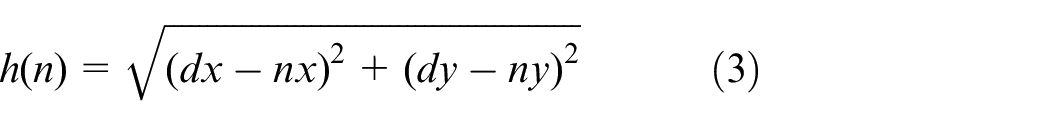
The A-star algorithm combines the advantages of breadth-first search from Dijkstra’s algorithm and greedy best-first search. It aims to minimize the number of nodes searched while guaranteeing the discovery of the optimal solution, thereby boosting efficiency of search.18–20 It utilizes a heuristic function

Where f(n) represents the evaluation cost from the start node to the target node,

In the first step of the A-star algorithm, the start node is placed into a priority queue with its
Precise path planning
Improvement
As previously mentioned, the A-star algorithm searches for the optimal path from a given source to the destination via a tree structure. Tree nodes are explored based on their f(n) values, and the A-star algorithm utilizes
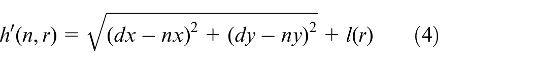

Where,
Schematic diagram of the extension line.
The unknown path cost estimation function
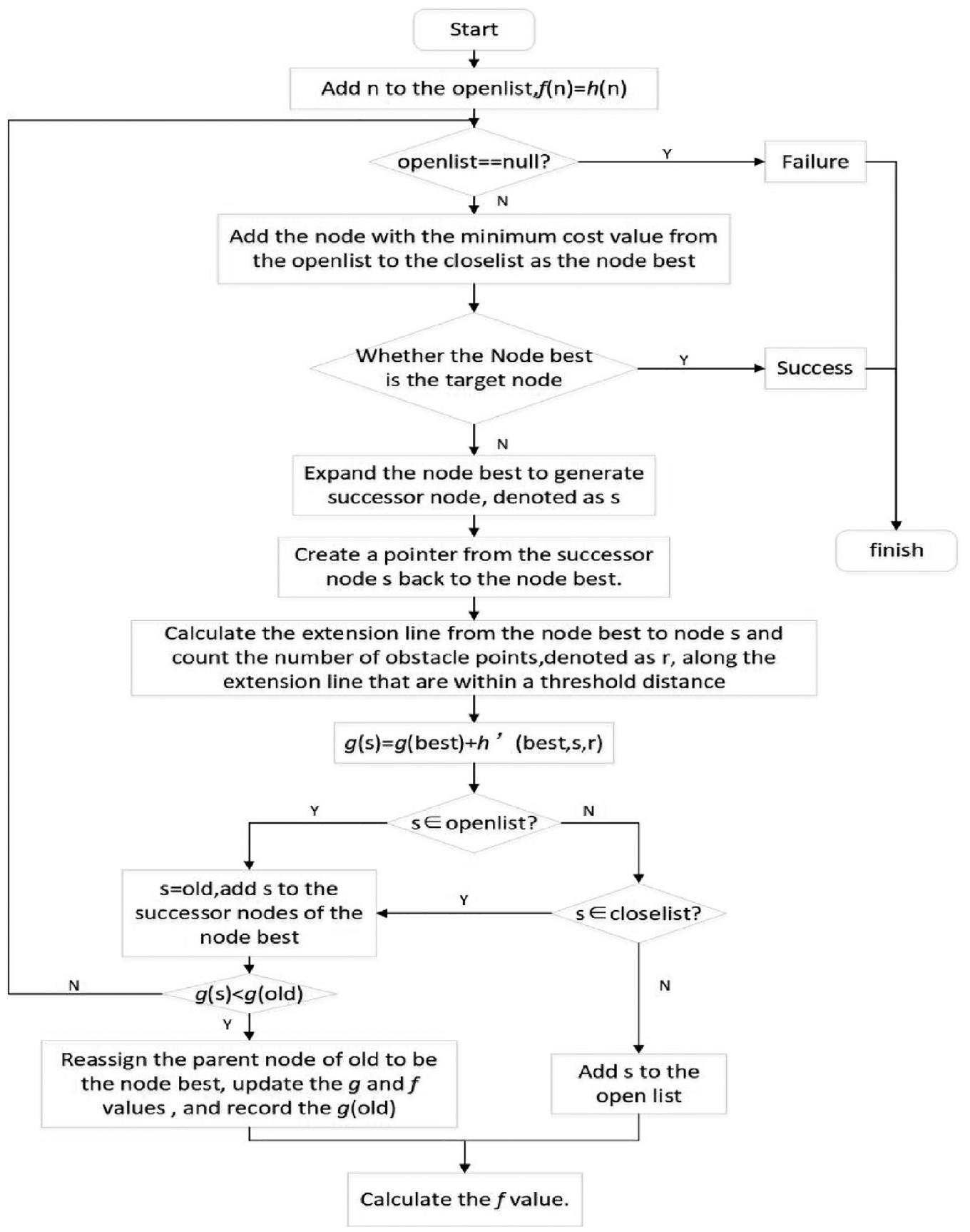
Flowchart of the improved A-star algorithm.
Locally zooming on the map
In path planning, the accuracy of the map is very important for generating the optimal path. In a grid map, dividing the map into cells allows for easy representation of obstacles, feasible areas, as well as other information. However, when the map is not precise enough, the generated path may also be not precise enough. In such cases, zooming on the map is a viable solution. However, there are also drawbacks to zooming on the map. Zooming on the map can increase computation time as more cells need to be calculated. Additionally, zooming on the map can occupy more memory. Thus, this paper achieves precise path planning by locally zooming on the map, thereby reducing calculated quantity and minimizing computation time.
Locally zooming on the map refers to enlarging the area adjacent to the derived path in the map. In this area, the cells will become smaller, and the contours and ranges of obstacles will become more refined as well, thereby enhancing the accuracy of the map and generating shorter paths. Thus, in scenarios that require high-precision maps, locally zooming on the map is a worthwhile consideration. For instance, in robot navigation, the robot may have to avoid some small obstacles. If locally zooming on the map is not performed at this time, there is a possibility that these obstacles may be overlooked.
When performing local zooming on a grid map, it is important to give consideration to the limitations of the grid size. The grid size refers to the size of the grid cell, usually expressed as the length or width. To guarantee that the zoomed-in grid map can still accurately represent environmental features and maintain consistency with the actual environment, the minimum value of the grid size should not be smaller than the size of the small vehicle. This is because when a grid map is used for path planning, navigation and other applications, it is crucial to guarantee that the small vehicle can accurately represent and move within the grid map. If the grid size is smaller than the size of the small vehicle, it may result in the small vehicle being unable to traverse the planned path, thereby affecting the accuracy and safety of the path planning. Thus, when performing local zooming on a grid map, it is essential to determine the appropriate grid size based on the size of the small vehicle and guarantee that the minimum grid size is not smaller than the size of the small vehicle, in a bid to guarantee the accuracy and reliability of the grid map.
In this paper, the improved A-star algorithm is used to plan the path of maps with different enlargement dimensions. Figures 3 to 5 are maps with different enlargement dimensions.For demonstration purposes, some of the images used in this paper are fully zoomed maps.
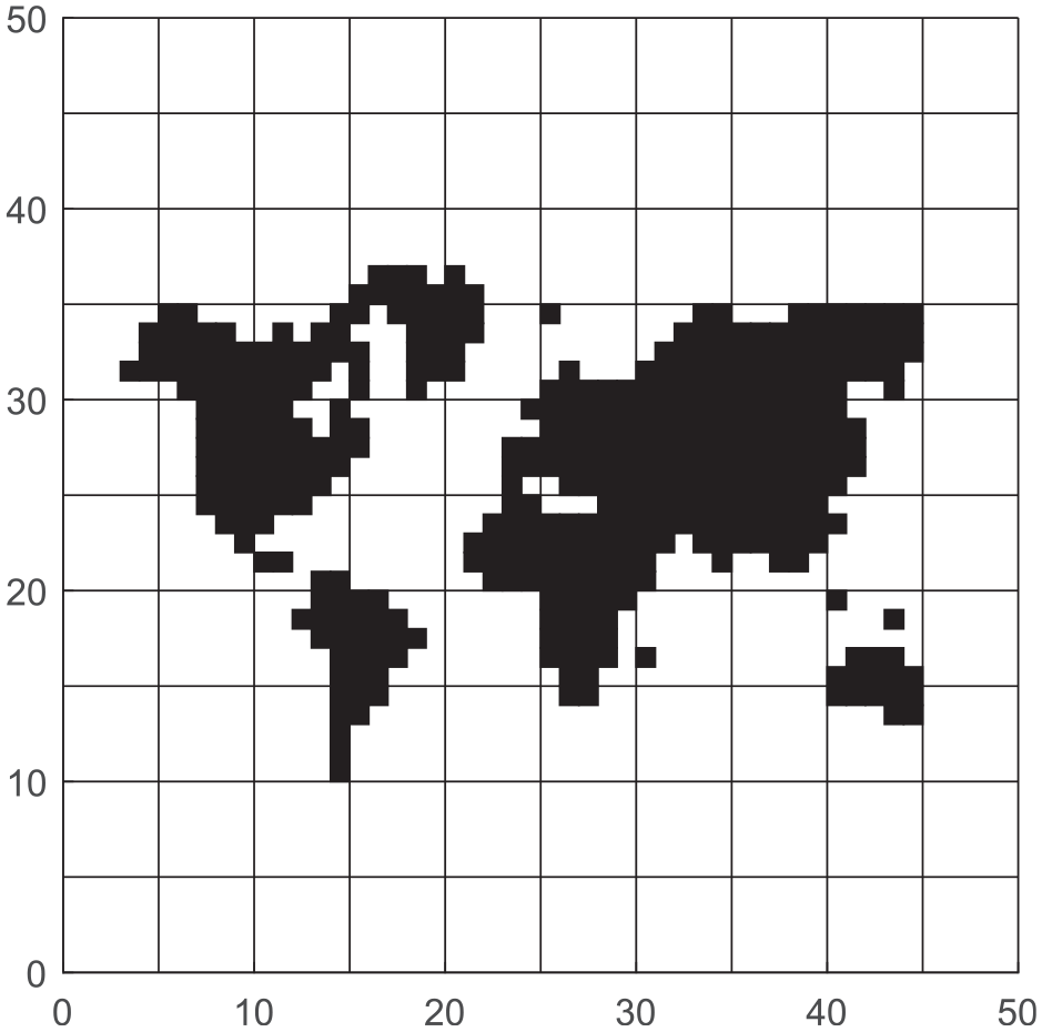
A 50 × 50 map.
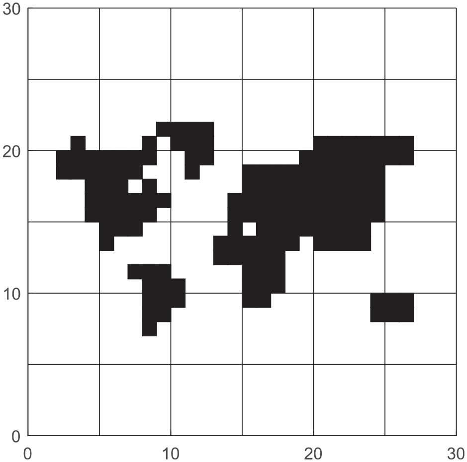
A 30 × 30 map.
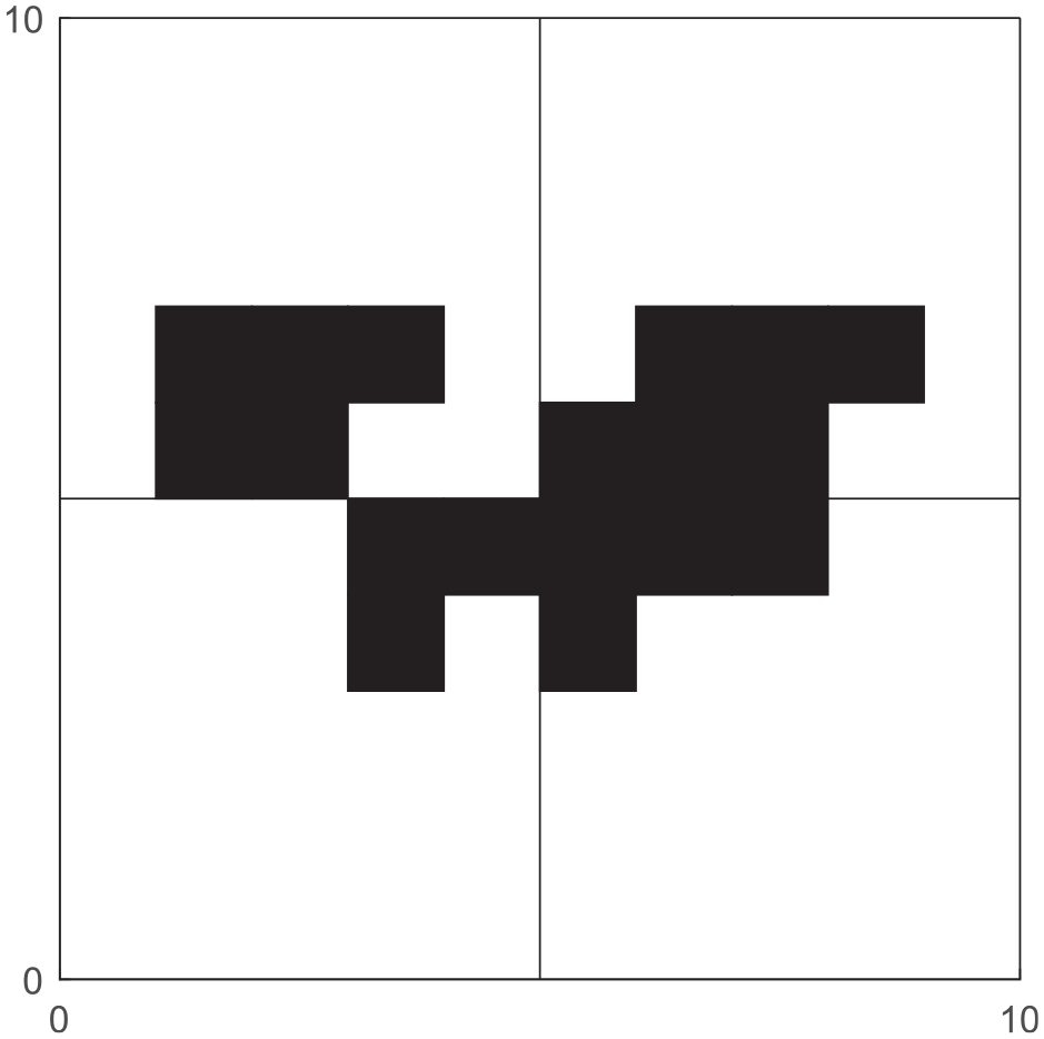
A 10 × 10 map.
Simulation of path planning
General case
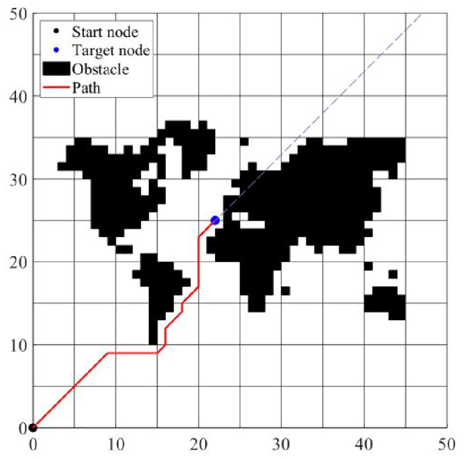
To validate the effectiveness and feasibility of this strategy, this study conducted an simulation of path planning on a specific map by way of an improved A-star algorithm. In the simulation of path planning, black grids represent obstacle areas, while white grids represent free passage areas. The red line indicates the planned path.
Path planning was conducted on maps with different dimensions, and Figures 6 to 8 represent different results of path planning. Figure 9 represents the results of local zoom path planning. The evaluation indexes for comparing the pros and cons of different zoomed dimensions were based on path length and operation time. The comparative results are displayed in Table 1.
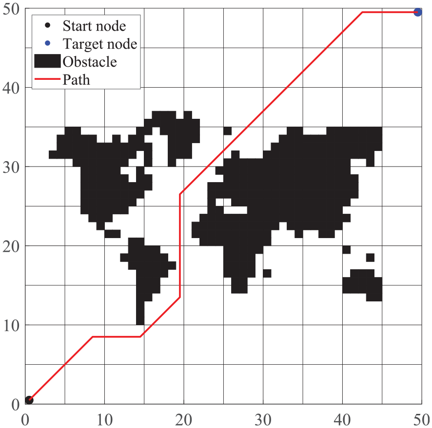
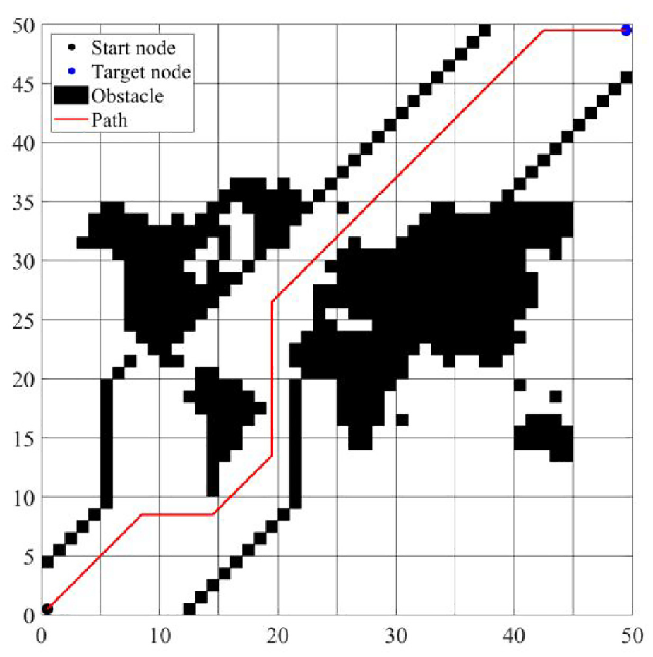
Result of path planning on a 50×50 map.
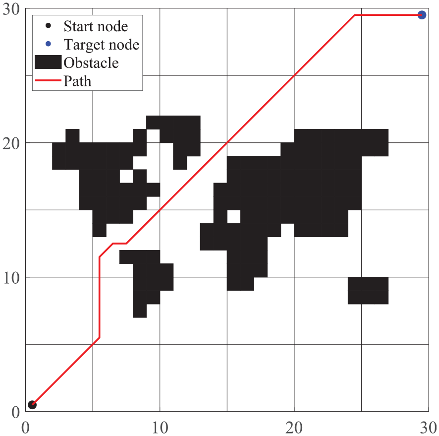
Result of path planning on a 30×30 map.
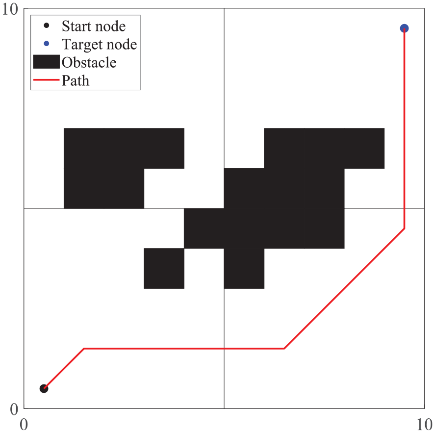
Result of path planning on a 10 × 10 map.
Result of local zoom path planning.
Results of path plannings on maps with different zoomed dimensions.
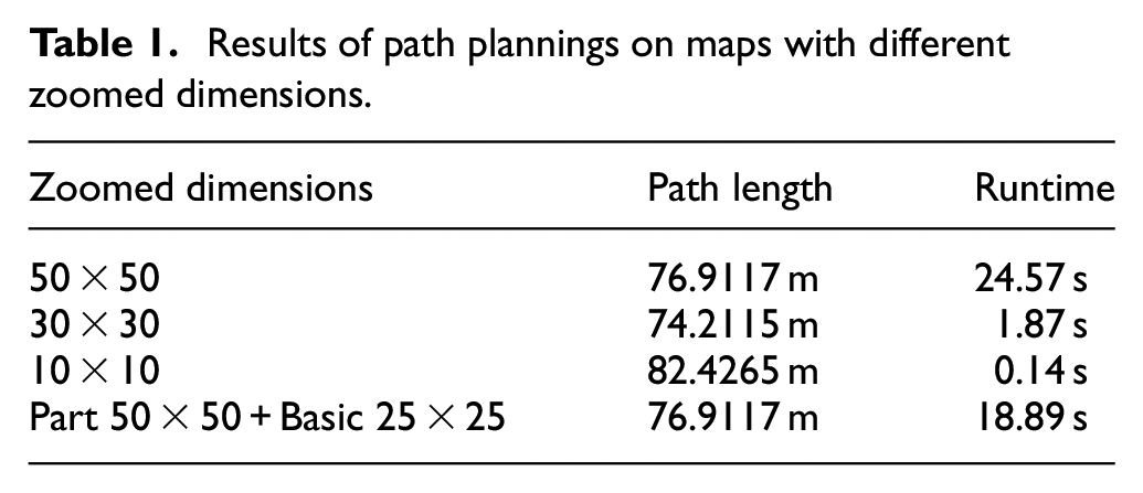
It can be observed from Figures 6 to 8 that as the zoomed dimensions of the map increase, the grid map will become closer to the original map, with more complete obstacles, and the paths derived from the path planning are closer to the actual situation. From Table 1, it can be learned that the path length on the map with the zoomed dimensions of 50 × 50 is shorter than the path length on the map with the zoomed dimensions of 10 × 10. Although the path on the map with the zoomed dimensions of 30 × 30 is shorter, there are impassable obstacles along that path in the actual map. It can be learned that the proposed method of locally zooming on the map in this paper can shorten the path distance while guaranteeing that the path is passable. The length of the path obtained by locally enlarging the 50 × 50 map is equal to that obtained by enlarging the 50 × 50 map, but the time is shortened by more than 23%. In the above map scenario, the algorithm has a shorter run time compared to the traditional A-star algorithm. However, in terms of path length, the algorithm has no significant advantage over A-star algorithms that combine other algorithms (e.g. A-star algorithms that combine particle swarm algorithms).21,22
Special case 1
Figure 10 represents the simulation map, while Figures 11 and 12, and 13 depict the path planning results for different zoomed dimensions. In the map illustrated in Figure 10, the locally zoomed A-star algorithm can not only be used to find the shortest path but accurately determine whether there are passable paths within the obstacle areas, thereby reducing the path length to a greatest extent. The larger the zoomed size, the more remarkable the effect of path planning.

Special case 1.
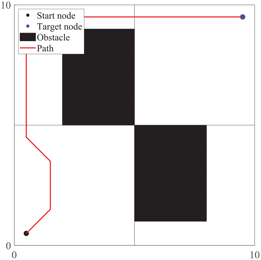
Result of path planning on a 10×10 map.
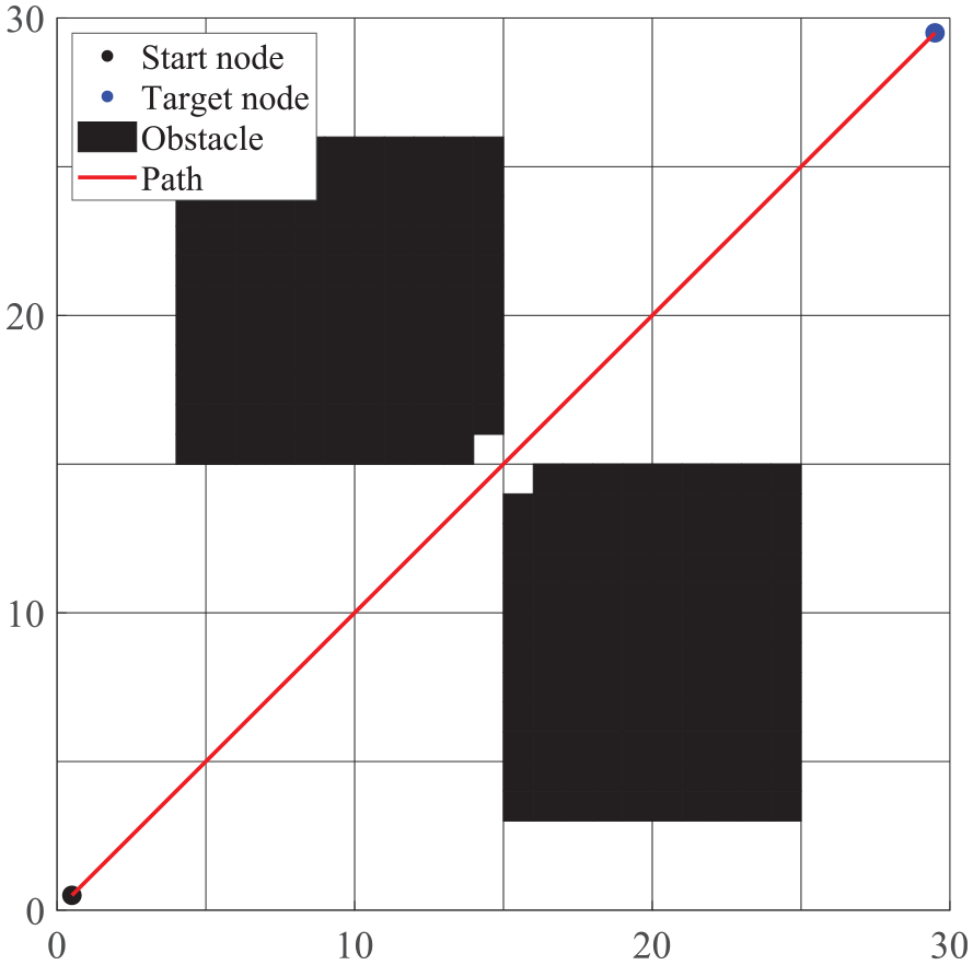
Result of path planning on a 30×30 map.
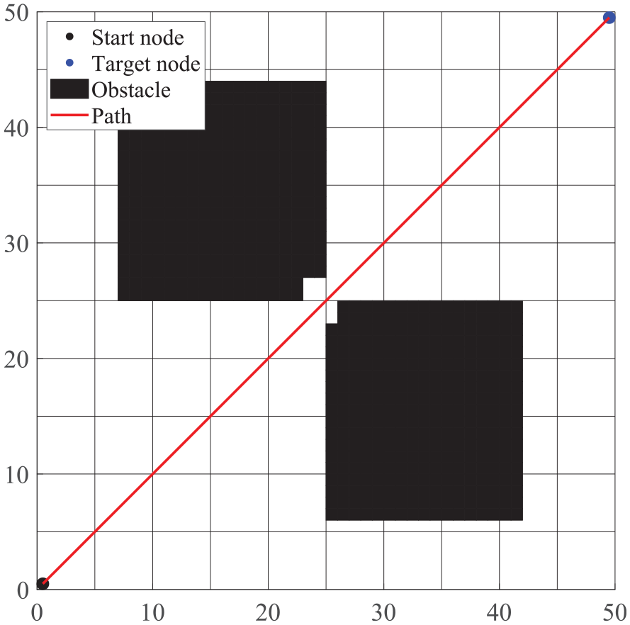
Result of path planning on a 50×50 map.
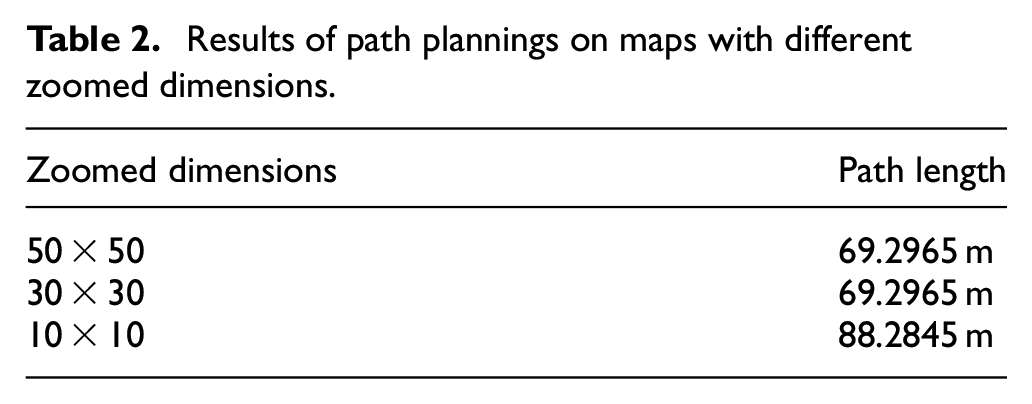
Table 2 presents a performance index comparison of three paths from the starting point to the ending point in grid environments of different dimensions. Table 2 shows that the locally zoomed A-star path planning algorithm can reduce the path length in an effective manner. The result of path planning in Figure 11 is relatively long, which is caused by path distortion. The path planning results in Figures 12 and 13 are 21% shorter compared to Figure 11, which shows that the algorithm can effectively shorten the path lengths while maintaining the authenticity of the maps.
Results of path plannings on maps with different zoomed dimensions.
Special case 2
Figure 14 represents another simulation map, while Figures 15 and 16, and 17 depict the results of path plannings for different zoomed dimensions. In the map illustrated in Figure 14, the locally zoomed A-star algorithm can more accurately determine the range of obstacle areas, avoiding the problem of the path derived by path planning meeting small obstacles during actual travel.

Special case 2.
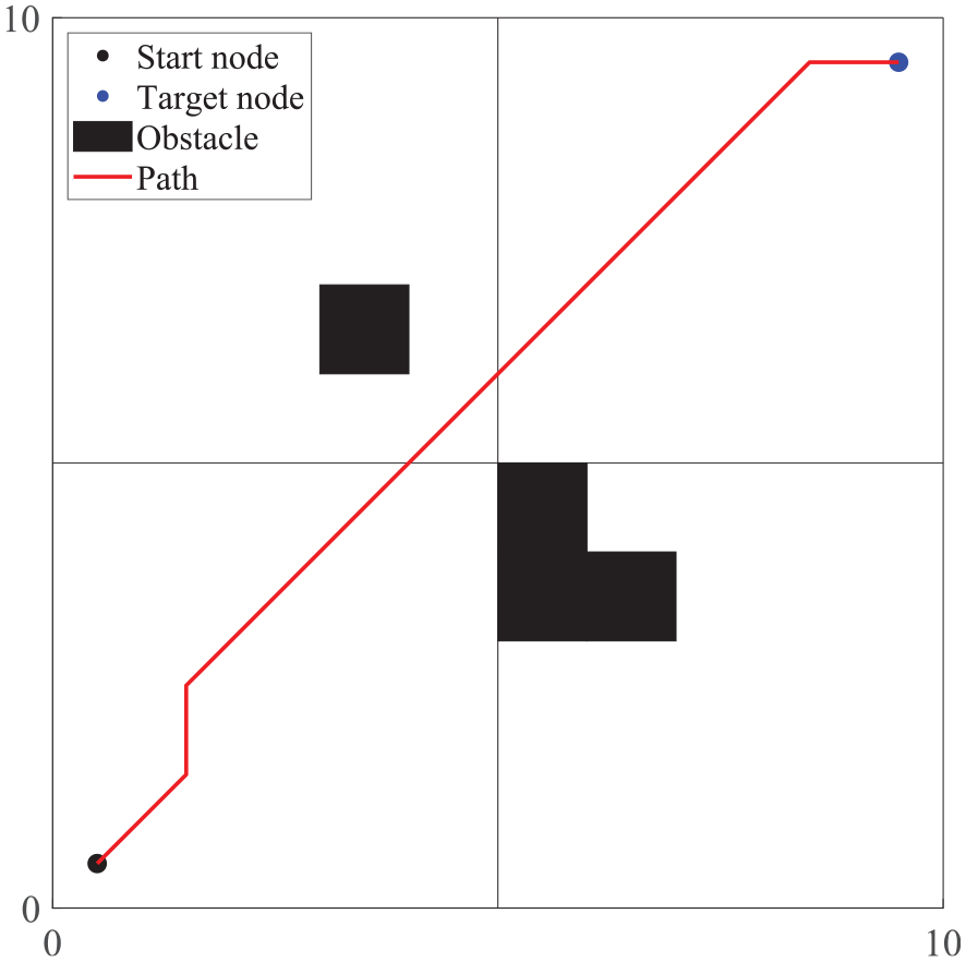
Result of path planning on a 10×10 map.
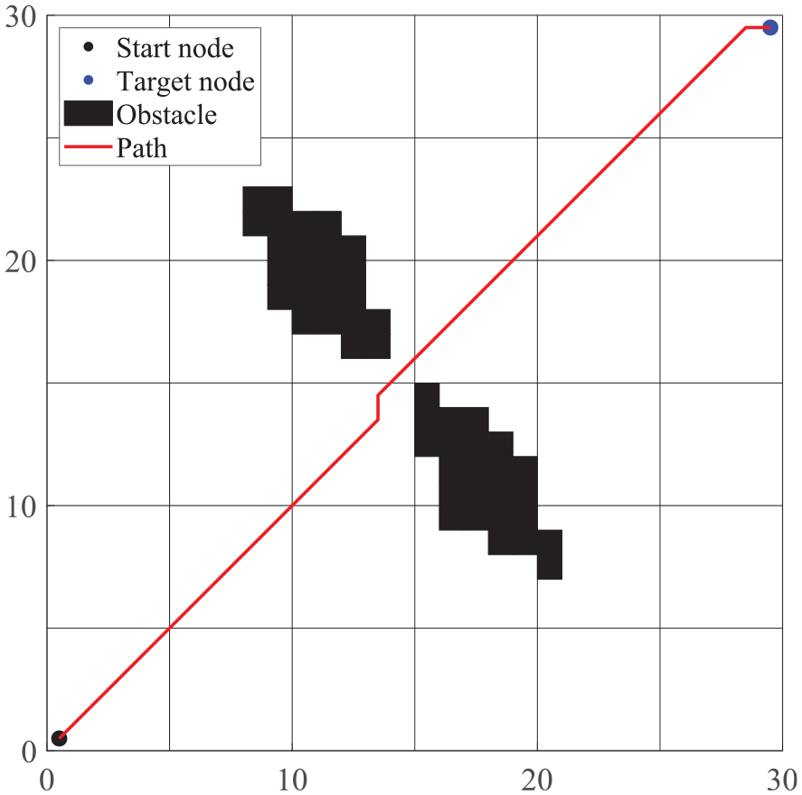
Result of path planning on a 30×30 map.
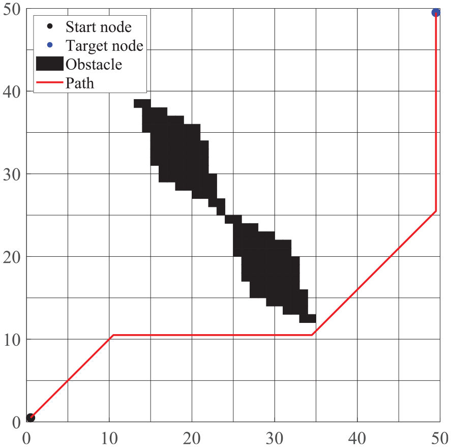
Result of path planning on a 50×50 map.
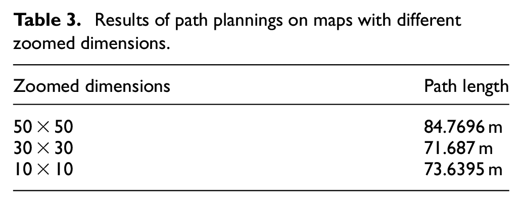
Table 3 presents a performance index comparison of three paths from the starting point to the ending point in grid environments of different dimensions. From Table 3, it can be observed that locally zooming on the map avoids local distortion, which is the primary priority, followed by shortening the path length. Although path plannings in Figures 15 and 16 result in shorter lengths, the paths are distorted. On the other hand, the result of path planning in Figure 17, despite having a longer length, provides an authentic path that avoids collisions with obstacles in the actual scenario. This algorithm is capable of shortening the path length while guaranteeing that the map remains undistorted.
Results of path plannings on maps with different zoomed dimensions.
LQR control
Dynamic model
As exhibited in Figure 1, the robot or vehicle is simplified as a “two-wheel” model. Assuming that the front and rear wheels are identical, both lateral and longitudinal motion degrees of freedom are taken into account in this model. By analyzing the force distribution of the vehicle in the x-axis and z-axis directions in Figure 18, and assuming a fixed vehicle speed and small wheel steering angle, the following equation can be derived:


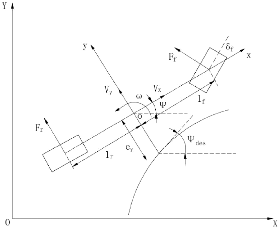
Vehicle dynamics and path tracking error model.
In the equation, m represents the mass of the small vehicle; a represents the lateral acceleration of the car;
Under the condition of small lateral acceleration, the lateral force and drift angle of the tire are regarded to be approximately proportional. Assuming that the cornering stiffness and rotation angle of the wheels on both sides of the same axis are equal, and the cornering stiffness of the front and rear wheels are respectively denoted as
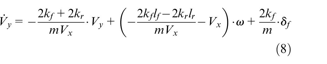
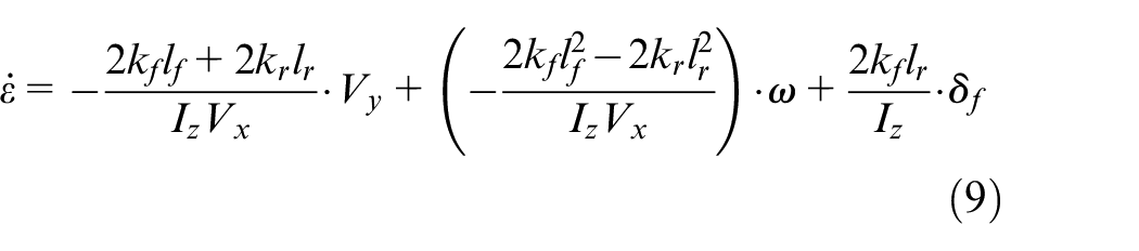
Where,
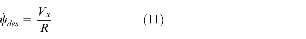
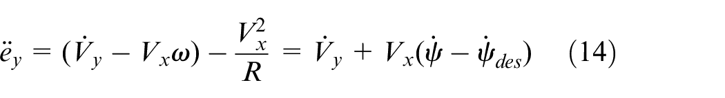
This paper controls the small vehicle with two types of errors, namely distance deviation and course deviation, as displayed in Figure 18. The distance deviation

Where, Ψ represents the course angle of the car, and
For the distance deviation
The required actual acceleration is:

Then, the following equation can be derived:

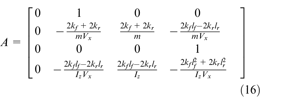
Based on the above equation, the state-space equation can be derived:

Where the A matrix is:
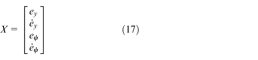
The quantity of state is:
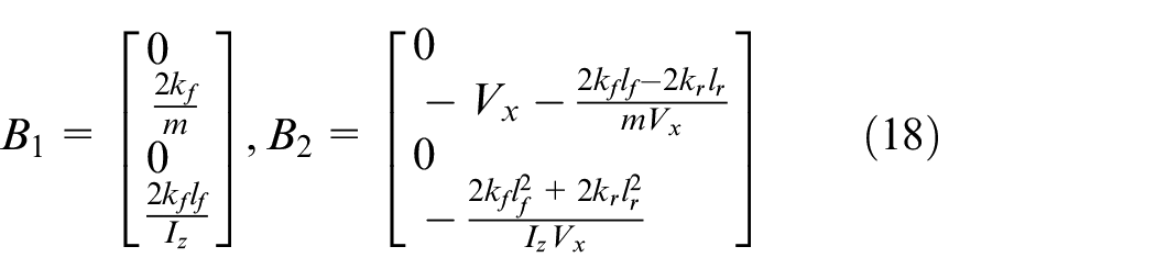
And the

Design of LQR controller
The design of the LQR controller is based on optimal control theory, which adjusts the system state by calculating weight matrices to achieve optimal control in the control system. An autonomous driving lateral motion controller is designed in line with LQR control theory. The LQR control flowchart is shown in Figure 19. Firstly, the performance index equation of the control system is determined, namely24,25:
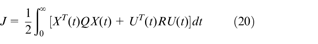
Where Q and R represent the weighting matrices of the controller.
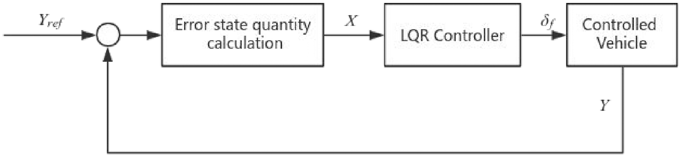
LQR control flowchart.
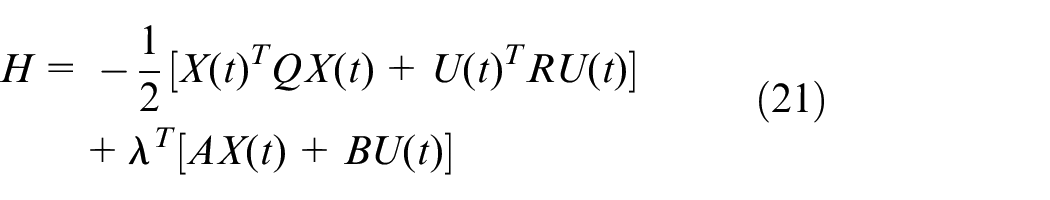
The LQR controller is targeted to minimize the value of the equation above. From this, the Hamiltonian function is constructed as below:
By taking the derivative and calculating the extremum of the equation above, the following equation can be derived:

Where

Where
Design of feedforward controller
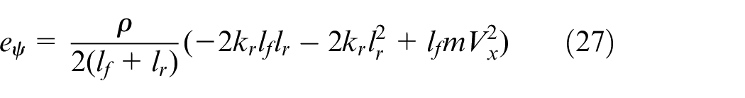
By substituting equation (23) into equation (15), the following equation can be derived26,27:

From equation (24), it can be observed that the system contains steady-state errors, meaning that both lateral error and course angle error cannot converge to zero simultaneously. Thus, considering the feedback control law of the front wheels, an additional feedforward term is added to guarantee that the lateral error can converge to zero. Let the steering angle of front wheels output by the feedforward control be

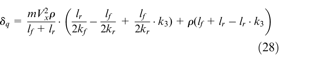
By substituting equation (25) into equation (15) and performing a Laplace transformation and calculating the extremum, the equations for the distance deviation and course deviation can be derived:
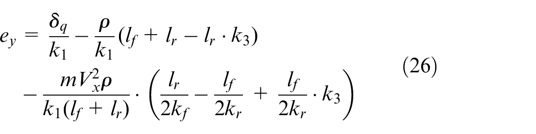
Where
Since the steady-state error of the distance deviation can be compensated for by feedforward control, this paper designs the feedforward control law based on equation (26), namely:
Improvement of LQR controller
In the traditional LQR controller, the robot does not take into account the special cases at the turning point when tracking the path, which makes the robot prone to instability or generating significant path deviation during rapid turns. To address this issue, this paper brings forward an improved LQR controller strategy that can enhance the stability and path tracking accuracy of the robot by introducing a deceleration mechanism at the turning point. When the robot is about to enter the turning point, the position of the turning point is detected first by monitoring the changes in path curvature. The curvature change at the turning point is significant. Thus, this characteristic can be utilized to determine when the robot is about to enter the turning point. Once the turning point is detected, the robot will slow down in line with a pre-defined deceleration strategy to guarantee a more stable turning.
In the phase of deceleration adjustment, we slow down the robot’s forward motion by adjusting the control input. This can be achieved by decreasing the gain of the controller output to reduce the turning speed of the robot. Simultaneously, we can also adjust the control input based on the degree of curvature at the turning point and the curvature of the path to better adapt to different turning conditions. The state space equation for adding the deceleration mechanism is:

The expression for the deceleration mechanism is:

Where the acceleration
After successfully navigating through the turning point, the robot’s speed will gradually return to its original velocity and control input to continue tracking the target path. The introduction of this deceleration adjustment strategy not merely enhances the stability and control precision of the robot at the turning point, but lowers the risk of collisions with the environment, thereby enhancing overall safety. The equation for velocity recovery is:

Where the acceleration a is constant.
Simulation test and analysis
To validate the design scheme of this paper, MATLAB simulation is used herein to test the designed controller, and the parameters of the vehicle are listed in Table 4. The whole LQR control simulation process includes controller part, dynamics part, trajectory part and vehicle state update part. The section concerning the controller addresses the linearization of the model for vehicle dynamics and control using LQR. The dynamics model uses the model described in section 5.1. The trajectory part is used to calculate the lateral deviation of the simulation process and can be used for error calculation in the controller section. The section responsible for updating the state of the vehicle computes the new condition based on the control inputs. For comparative analysis, this paper performs simulation tests on the paths planned in Section 4.1 by means of both traditional LQR control and improved LQR control. The initial velocities of the small vehicle in the x-axis and y-axis directions are set to 15 m/s, and the dimensions of the map are 50 m in length and width.
Main parameters of the vehicle.
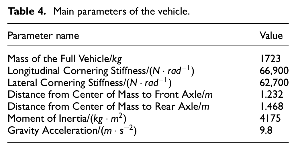
Figure 20 demonstrates the tracking performance of the vehicle under the action of two controllers. It can be observed that both controllers are capable of tracking the reference path and guaranteeing that the tracking error remains within an acceptable range. However, the improved LQR controller exhibits superior tracking performance with regard to the target path.
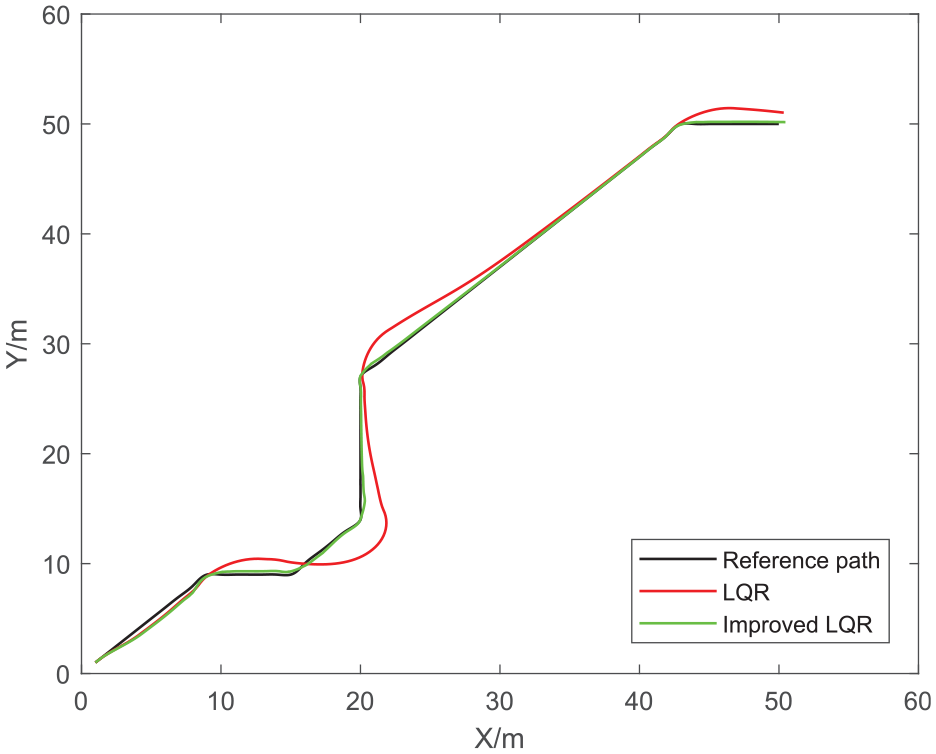
Tracking results of reference path.
Figures 21 and 22 give a precise depiction of the lateral deviation between the actual path of the vehicle and the reference path. The improved LQR feedforward controller exhibits superior tracking performance, with a maximum lateral deviation of less than 0.55 m and a runtime of 10.6 s; In contrast, the LQR feedforward controller shows lower tracking accuracy, with a maximum lateral deviation of up to 2.5 m and a runtime of 5.3 s. It can be observed that although the runtime of the improved LQR feedforward controller has doubled, it has higher tracking accuracy and better control performance. The maximum lateral error is decreased by 78%. The average error of the conventional LQR control was 0.7583 m and the average error of the improved LQR control was 0.1517 m. The average error was reduced by 80%.
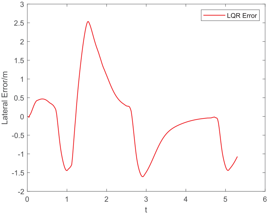
Error of LQR controller.
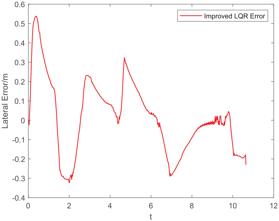
Error of improved LQR controller.
Conclusion
This paper performs path planning based on the improved A-star algorithm and locally zooming on the map method. Building upon the traditional A-star algorithm as the theoretical foundation, an additional unknown path cost estimation function is incorporated to measure the predictive evaluation cost. Subsequently, the obstacles near the path are locally zoomed, followed by another round of path planning to reach more accurate planning results. The final time required for path planning was reduced by 23% in the map shown in Figure 23, and the path distance was reduced by 21% in the map shown in Figure 10. In the map shown in Figure 14, although the path length was not reduced, a more accurate path was found and collisions with obstacles were avoided.

Original map.
Subsequently, the improved lateral LQR algorithm is employed to design a tracking controller, enabling real-time tracking of the locally planned path as well as path points. This paper brings forward an improved LQR controller strategy that incorporates a deceleration mechanism at turning points, enhancing the stability and path tracking accuracy of the robot to a great extent. The final improved LQR control reduces the average error by 80% compared to the conventional LQR control.
Footnotes
Declaration of conflicting interests
The author(s) declared no potential conflicts of interest with respect to the research, authorship, and/or publication of this article.
Funding
The author(s) received no financial support for the research, authorship, and/or publication of this article.
Data sharing agreement
The datasets used and/or analyzed during the current study are available from the corresponding author on reasonable request.