Numerical algorithm for hypersonic vehicle optimal flight control

Abstract

We consider a hypersonic vehicle optimal flight control problem. The problem is modeled as an optimal control problem of switched systems (OCPSS), which can become a parameter optimization problem (POP). Following that, to achieve the globally optimal solution of the POP, an improved continuous filled function (CFF) algorithm including one adjusting parameter is proposed based on a penalty function, in which the CFF is differentiable, excludes logarithmic terms or exponential terms, and does not require to minimize the cost function. Numerical results show that the proposed algorithm is effective.

Introduction

The hypersonic vehicles has been attracting researchers because of the two successful flight tests of the X–43A conducted by National Aeronautics and Space Administration. ¹ The correlation technologies, such as integrated design technology, aerodynamics and aeroheating technology, high-temperature long-time thermal protection technology, and hypersonic propulsive technology, etc, have been extensively investigated. ² The guidance and control technology is a crucial technologies of hypersonic vehicles, which is to ensure their efficiency and feasibility. ³ However, the guidance and control technology must have high precision, high reliability, and strong adaptability.^4,5 Thus, many key problems, such as reentry guidance, rapid trajectory changing, trajectory optimization, flight guidance, and so on, urgently need to be addressed. ⁶ In order to achieve these goals, the flight path optimization is essential for hypersonic vehicles. ⁷

The optimal control problem of switched systems (OCPSS) includes choosing a control input and a switching sequence such that a system performance is optimized. ⁸ It is still a challenging problem to obtain a solution of the OCPSS. ⁹ To overcome the challenging, maximum principle (MP) and dynamic programing (DP) are extended to switched systems. ¹⁰ By using the MP, one can solve the simple OCPSS analytically. But, in application, the problem may be too complex and big, which leads to the use of a modern computer is unavoidable. ¹¹ For the DP, it require to solve a Hamilton-Jacobi-Bellman (HJB) equation. Although the HJB equation has already had a firm theoretical foundation to solve, the OCPSS can not be solved analytically in general. ¹² Some numerical algorithms have been proposed for solving the OCPSS. ¹³ One well-known algorithm is the bi-level optimization method. ¹⁴ The other alternative approach is the method based on the embedding technique.^15,16 In addition, an improved bi-level optimization method ¹⁷ and an improved mixed-integer optimal control approach ¹⁸ have also been developed for solving the OCPSS. Unfortunately, the solutions obtained by using these methods are usually locally optimal solutions instead of globally optimal solution, and the amount of calculation and the convergence rate of these methods are still less encouraged.

Recently, to solve global optimization problems, some algorithms have been developed. Generally speaking, we can divide these algorithms into two categories: deterministic algorithm (DA) and probabilistic algorithm (PA). The DA involves the trajectory approach, ¹⁹ auxiliary function approach, ²⁰ covering approach, ²¹ etc. Simulated annealing algorithm, ²² genetic algorithm, ²³ differential evolution, ²⁴ and particle swarm optimization ²⁵ are several typical algorithms of the PA. Note that most of the optimization problems usually own many local minimizers in practical applications. Thus, the key of obtaining a global solution is choosing a method to escape from the present local solution. As a typical DA, the CFF is designed for global optimization problems. ²⁶ However, the existing CFF either require more than an adjusting parameter, ²⁷ involve ill-conditioned term (logarithmic terms or exponential terms), ²⁸ or are non-differentiable (even discontinuous). ¹⁹ In addition, the general framework of the CFF implies that the local solution of the CFF is usually not the local solution of the original optimization problem, and a better local solution achieved require to solve the original optimization problem. Thus, if the CCF has the same local solution of the original optimization problem, and the local solution is better than the present solution of the original optimization problem, then a local solution of the CFF will be a better local solution of the original optimization problem. Then, the efficiency of the CFF will increase significantly.

In the route planning problem for a hypersonic vehicle, the optimal speed cruise and the periodic cruise are two common flight modes. However, compared with the optimal speed cruise, the periodic cruise can save more fuel. Then, to enhance the flight performance, many researchers have investigated the periodic cruise. The flight trajectory of a hypersonic vehicle with the periodic cruise are separated into two components: rarefied atmosphere and condensed atmosphere. Then, the route planning problem of a hypersonic vehicle with the periodic cruise can be modeled as an OCPSS with some inequality constraints and terminal constraints. To obtain a numerical solution, based on the time-scaling transformation and some auxiliary piecewise-constant functions, the OCPSS is transformed into a POP. Solutions obtained by using the gradient-based algorithms are usually locally optimal solutions instead of globally optimal solution. In addition, the amount of calculation and the convergence rate of the gradient-based algorithms are also less encouraged. To avoid the shortcomings of the gradient-based algorithms and the conventional CFF, a penalty function-based improved CFF algorithm is developed for solving the POP. It should be pointed out that the improved CFF is differentiable, only requires a adjusting parameter, and excludes logarithmic terms or exponential terms. More importantly, any one local solution of the improved CFF is a better local solution of the original parameter optimization problem. Thus, the penalty function-based improved CFF algorithm does not require to minimize the cost function. In addition, compared with the gradient-based algorithms, the penalty function-based improved CFF algorithm is a global optimization algorithm, which takes less time and converges faster. Finally, numerical results illustrate the effectiveness of the proposed method.

The main contributions of this article can be summarized as follows:

• Hypersonic vehicle optimal flight control is modeled as an OCPSS.

• An improved CFF algorithm is developed for solving the OCPSS.

• Numerical results show that the proposed method is effective and robust.

The rest of this paper is organized as follows. The hypersonic vehicle optimal flight control problem is presented in Section 2. An equivalent OCPSS is obtained in Section 3. In Section 4, the OCPSS is written as a POP. Then, an improved CFF is developed in Section 5. By numerical simulation, Section 6 illustrates the effectiveness of the proposed method.

Notations: $x(t)$ and $y(t)$ present the longitudinal coordinates of the hypersonic vehicle; $m(t)$ presents the mass of the hypersonic vehicle; $F(t)$ presents the thrust of the hypersonic vehicle; $a$ is a constant, which presents the effective exhaust velocity; $b$ is a constant, which presents the thrust coefficient; $g$ presents the gravitational acceleration; ${\eta }_1\left(t\right)$ presents the elevator deflection angle; ${\eta }_2\left(t\right)$ presents the throttle opening; $T_1$ and $S_1$ present the air resistance and the lift of the hypersonic vehicle in the rarefied atmosphere, respectively; $T_2$ and $S_2$ present the air resistance and the lift of the hypersonic vehicle in the condensed atmosphere, respectively; and $\upsilon$ presents the attack angle; OCPSS presents optimal control problem of switched systems; POP presents parameter optimization problem; CFF presents continuous filled function; MP presents maximum principle; DP presents dynamic programing; DA presents deterministic algorithm; and PA presents probabilistic algorithm.

Problem description

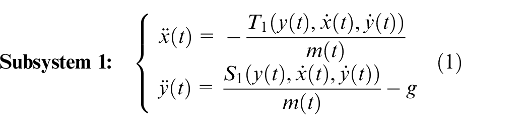
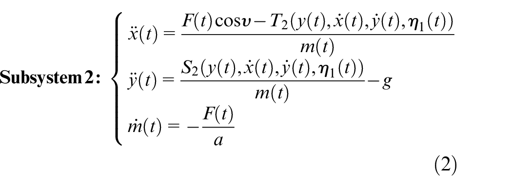
In the route planning problem of a hypersonic vehicle, the optimal speed cruise and the periodic cruise are two common flight modes. However, compared with the optimal speed cruise, the periodic cruise can save more fuel. Thus, to improve the flight performance, many researchers have investigated the periodic cruise. In general, we can divide the flight trajectory of a hypersonic vehicle with the periodic cruise into two components: rarefied atmosphere and condensed atmosphere. Then, the dynamic process of the hypersonic vehicle with the periodic cruise described by Snyman and Fatti, ²⁹ Chuang and Morimoto, ³⁰ and Hou and Ding ³⁶ can be modeled as a switched dynamic system:

$$\mathbf{Subsystem}1:\{\begin{array}{c}\begin{array}{c}\stackrel{··}{x}\left(t\right)=-\frac{T_1(y\left(t\right),\stackrel{·}{x}\left(t\right),\stackrel{·}{y}\left(t\right))}{m\left(t\right)}\hfill \\ \multicolumn{1}{c}{\stackrel{··}{y}\left(t\right)=\frac{S_1(y\left(t\right),\stackrel{·}{x}\left(t\right),\stackrel{·}{y}\left(t\right))}{m\left(t\right)}-g}\end{array}\hfill \end{array}$$

(1)

$$\mathbf{Subsystem}2:\{\begin{array}{c}\begin{array}{c}\stackrel{··}{x}\left(t\right)=\frac{F\left(t\right)\cos \upsilon -T_2(y\left(t\right),\stackrel{·}{x}\left(t\right),\stackrel{·}{y}\left(t\right),{\eta }_1\left(t\right))}{m\left(t\right)}\hfill \\ \multicolumn{1}{c}{\stackrel{··}{y}\left(t\right)=\frac{S_2(y\left(t\right),\stackrel{·}{x}\left(t\right),\stackrel{·}{y}\left(t\right),{\eta }_1\left(t\right))}{m\left(t\right)}-g}\\ \multicolumn{1}{c}{\stackrel{·}{m}\left(t\right)=-\frac{F\left(t\right)}{a}}\end{array}\hfill \end{array}$$

(2)

where

$$F\left(t\right)=b{\eta }_2\left(t\right);$$

(3)

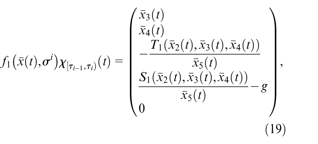
Subsystems 1 and 2 present the hypersonic vehicle flying in the rarefied atmosphere and the condensed atmosphere, respectively; $x(t)$ and $y(t)$ present the longitudinal coordinates of the hypersonic vehicle; $m(t)$ presents the mass of the hypersonic vehicle; $F(t)$ presents the thrust of the hypersonic vehicle; $a$ is a constant, which presents the effective exhaust velocity; $b$ is a constant, which presents the thrust coefficient; $g$ presents the gravitational acceleration; ${\eta }_1\left(t\right)$ presents the elevator deflection angle; ${\eta }_2\left(t\right)$ presents the throttle opening satisfying

$$0\le {\eta }_2\left(t\right)\le 1;$$

(4)

$T_1(y\left(t\right),\stackrel{·}{x}\left(t\right),\stackrel{·}{y}\left(t\right))$ and $S_1(y\left(t\right),\stackrel{·}{x}\left(t\right),\stackrel{·}{y}\left(t\right))$ present the air resistance and the lift of the hypersonic vehicle in the rarefied atmosphere, respectively; $T_2(y\left(t\right),\stackrel{·}{x}\left(t\right),\stackrel{·}{y}\left(t\right),{\eta }_1\left(t\right))$ and $S_2(y\left(t\right),\stackrel{·}{x}\left(t\right),\stackrel{·}{y}\left(t\right),{\eta }_1\left(t\right))$ present the air resistance and the lift of the hypersonic vehicle in the condensed atmosphere, respectively; and $\upsilon$ presents the attack angle.

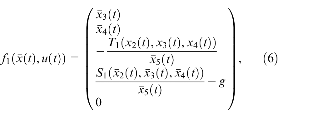
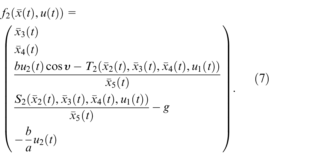
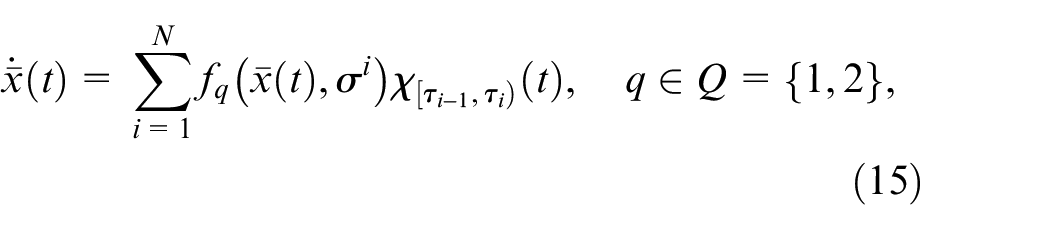
Let ${\overline{x}}_1\left(t\right)=x\left(t\right)$ , ${\overline{x}}_2\left(t\right)=y\left(t\right)$ , ${\overline{x}}_3\left(t\right)=\stackrel{·}{x}\left(t\right)$ , ${\overline{x}}_4\left(t\right)=\stackrel{·}{y}\left(t\right)$ , ${\overline{x}}_5\left(t\right)=m\left(t\right)$ , $u_1\left(t\right)={\eta }_1\left(t\right)$ , and $u_2\left(t\right)={\eta }_2\left(t\right)$ . Following that, with $\overline{x}\left(t\right)={[{\overline{x}}_1\left(t\right),{\overline{x}}_2\left(t\right),{\overline{x}}_3\left(t\right),{\overline{x}}_4\left(t\right),{\overline{x}}_5\left(t\right)]}^{\mathrm{T}}$ and $u\left(t\right)={[u_1\left(t\right),u_2\left(t\right)]}^{\mathrm{T}}$ , (1) and (2) becomes a switched system:

$$\stackrel{·}{\overline{x}}\left(t\right)=f_q(\overline{x}\left(t\right),u\left(t\right)),q\in Q=\{1,2\},$$

(5)

where

$$f_1(\overline{x}\left(t\right),u\left(t\right))=\left(\begin{array}{c}{\overline{x}}_3\left(t\right)\hfill \\ \multicolumn{1}{c}{{\overline{x}}_4\left(t\right)}\\ \multicolumn{1}{c}{-\frac{T_1({\overline{x}}_2\left(t\right),{\overline{x}}_3\left(t\right),{\overline{x}}_4\left(t\right))}{{\overline{x}}_5\left(t\right)}}\\ \multicolumn{1}{c}{\frac{S_1({\overline{x}}_2\left(t\right),{\overline{x}}_3\left(t\right),{\overline{x}}_4\left(t\right))}{{\overline{x}}_5\left(t\right)}-g}\\ \multicolumn{1}{c}{0}\end{array}\right),$$

(6)

$$\begin{array}{c}{f}_2(\overline{x}\left(t\right),u\left(t\right))=\hfill \\ \left(\begin{array}{c}{\overline{x}}_3\left(t\right)\hfill \\ \multicolumn{1}{c}{{\overline{x}}_4\left(t\right)}\\ \multicolumn{1}{c}{\frac{b{u}_2\left(t\right)\cos \upsilon -T_2({\overline{x}}_2\left(t\right),{\overline{x}}_3\left(t\right),{\overline{x}}_4\left(t\right),u_1\left(t\right))}{{\overline{x}}_5\left(t\right)}}\\ \multicolumn{1}{c}{\frac{S_2({\overline{x}}_2\left(t\right),{\overline{x}}_3\left(t\right),{\overline{x}}_4\left(t\right),u_1\left(t\right))}{{\overline{x}}_5\left(t\right)}-g}\\ \multicolumn{1}{c}{-\frac{b}{a}{u}_2\left(t\right)}\end{array}\right).\hfill \end{array}$$

(7)

Note that the elevator deflection angle ${\eta }_1(t)$ satisfies $-{25}^0\le {\eta }_1\left(t\right)\le {25}^0$ due to ${\eta }_1(t)$ being limited by mechanical structure, and the engine thrust depends on throttle opening ${\eta }_2(t)$ , where $0\le {\eta }_2\left(t\right)\le 1$ . Thus, the control input $u(t)$ satisfies the following continuous–time inequality constraints:

$$-{25}^0\le u_1(t)\le {25}^0,$$

(8)

$$0\le u_2(t)\le 1.$$

(9)

The main purpose of this paper is to maximize the flying distance of the hypersonic vehicle with fixed fuel by choosing the ignition time, the elevator deflection angle, and the throttle opening. Suppose that the initial condition is given by

$${\overline{x}}_1\left(t_0\right)={\overline{x}}_1^0,{\overline{x}}_2\left(t_0\right)={\overline{x}}_2^0,{\overline{x}}_3\left(t_0\right)={\overline{x}}_3^0,$$

$${\overline{x}}_4\left(t_0\right)={\overline{x}}_4^0,{\overline{x}}_5\left(t_0\right)={\overline{x}}_5^0,$$

(10)

the terminal constraint is given by

$$\overline{x}\left(t_f\right)={\overline{x}}_{t_f},$$

(11)

and the ignition time ${\tau }_i$ satisfies

$$t_0={\tau }_0\le {\tau }_1\le \cdots \le {\tau }_{N-1}\le {\tau }_N=t_f.$$

Here, $t_0$ denotes the initial time; $t_f$ denotes the terminal time; and ${\overline{x}}_{t_f}$ denotes the terminal state.

Define a switching sequence as follows:

$$\alpha =[({\tau }_0,q_0),({\tau }_1,q_1),\cdots ,({\tau }_N,q_N)].$$

Here, $N$ denotes the number of subsystem switches; $q_i\in Q$ for $i=0,1,\cdots ,N$ ; and $({\tau }_i,q_i)$ implies that for $i=0,1,\cdots ,N$ , the dynamics changes from subsystem $q_{i-1}$ to $q_i$ at time ${\tau }_i$ . Let $\mathrm{\Xi }$ denote the class of all switching sequence $\alpha$ corresponding to $\tau \in \mathrm{\Gamma }$ , where $\tau ={[{\tau }_1,\cdots ,{\tau }_{N-1}]}^{\mathrm{T}}$ and

$$\mathrm{\Gamma }=\{\tau \in R^{N-1}:t_0={\tau }_0\le {\tau }_1\le \cdots \le {\tau }_{N-1}\le {\tau }_N=t_f\}.$$

Thus, the set $\mathrm{\Xi }$ is depend on the ignition time ${\tau }_i$ , $i=0,\cdots ,N$ , the number $N$ of subsystem switches, and $q_i\in Q$ , $i=0,1,\cdots ,N$ . For a given $\tau \in \mathrm{\Gamma }$ , any continuous function $u\left(t\right):[0,t_f]\to R^2$ is referred to as an admissible control (AC). Let $U$ denote the class of all AC.

The problem of choosing the switching sequence, the elevator deflection angle, and the throttle opening may be given as the following OCPSS.

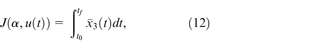
• Problem 1. For the system (5) with the initial condition (10), find a pair $(\alpha ,u\left(t\right))\in \mathrm{\Xi }\times U$ such that

$$J(\alpha ,u\left(t\right))={\int }_{t_0}^{t_f}{\overline{x}}_3\left(t\right)\mathrm{dt},$$

(12)

is maximized subject to the constraints (8), (9), and (11), where $t_f$ is a given terminal time and $\overline{x}\left(t_f\right)$ is a free terminal state.

Problem approximation and transformation

In this section, a simpler approximate problem corresponding to Problem 1 will be derived by restricting the control input to suitable piecewise constant functions and introducing some auxiliary piecewise-constant functions.

Problem approximation

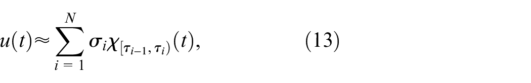
In this subsection, the following function is adopted to approximate $u(t)$ :

$$u\left(t\right)\approx \sum _{i=1}^N{\sigma }_i{\chi }_{[{\tau }_{i-1},{\tau }_i)}\left(t\right),$$

(13)

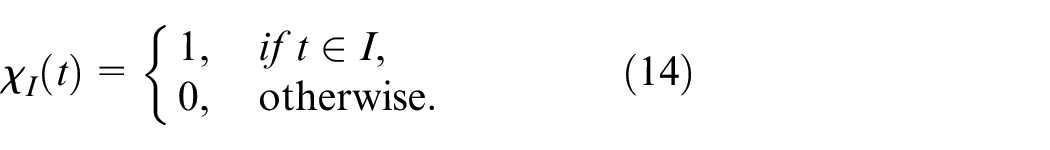
where ${\sigma }_i={[{\sigma }_i^1,{\sigma }_i^2]}^{\mathrm{T}}\in R^2$ , $i=1,\cdots ,N$ ; $N$ is a pre-given constant; and the function ${\chi }_I\left(t\right)$ is given by

$${\chi }_I\left(t\right)=\{\begin{array}{c}1,\mathrm{if}t\in I,\hfill \\ \multicolumn{1}{c}{0,\mathrm{otherwise}.}\end{array}$$

(14)

Define

$$\sigma ={[{\left({\sigma }_1\right)}^{\mathrm{T}},\cdots ,{\left({\sigma }_N\right)}^{\mathrm{T}}]}^{\mathrm{T}}.$$

Suppose that $\mathrm{\Omega }$ is the set of all $\sigma$ . By substituting the function (13) into the switched system (5), the constraints (8) and (9), and the cost function (12), we can define an approximate problem as follows:

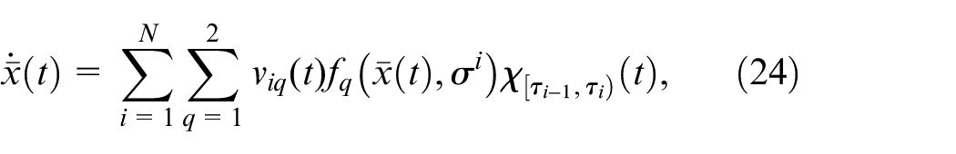
• Problem 2. Given the switched system:

$$\stackrel{·}{\overline{x}}\left(t\right)=\sum _{i=1}^N{f}_q(\overline{x}\left(t\right),{\sigma }^i){\chi }_{[{\tau }_{i-1},{\tau }_i)}\left(t\right),q\in Q=\{1,2\},$$

(15)

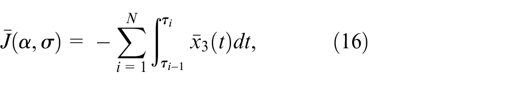
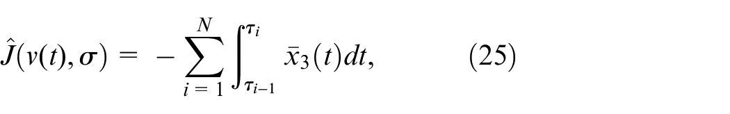
with (10), find a pair $(\alpha ,\sigma )\in \mathrm{\Xi }\times \mathrm{\Omega }$ such that

$$\overline{J}(\alpha ,\sigma )=-\sum _{i=1}^N{\int }_{{\tau }_{i-1}}^{{\tau }_i}{\overline{x}}_3\left(t\right)\mathrm{dt},$$

(16)

is minimized subject to the constraints

$$-{25}^0\le {\sigma }_i^1\le {25}^0,t\in [{\tau }_{i-1},{\tau }_i],i=1,\cdots ,N,$$

(17)

$$0\le {\sigma }_i^2\le 1,t\in [{\tau }_{i-1},{\tau }_i],$$

(18)

and the constraint (11), where

$$f_1(\overline{x}\left(t\right),{\sigma }^i){\chi }_{[{\tau }_{i-1},{\tau }_i)}\left(t\right)=\left(\begin{array}{c}{\overline{x}}_3\left(t\right)\hfill \\ \multicolumn{1}{c}{{\overline{x}}_4\left(t\right)}\\ \multicolumn{1}{c}{-\frac{T_1({\overline{x}}_2\left(t\right),{\overline{x}}_3\left(t\right),{\overline{x}}_4\left(t\right))}{{\overline{x}}_5\left(t\right)}}\\ \multicolumn{1}{c}{\frac{S_1({\overline{x}}_2\left(t\right),{\overline{x}}_3\left(t\right),{\overline{x}}_4\left(t\right))}{{\overline{x}}_5\left(t\right)}-g}\\ \multicolumn{1}{c}{0}\end{array}\right),$$

(19)

$$\begin{array}{c}{f}_2(\overline{x}\left(t\right),{\sigma }^i){\chi }_{[{\tau }_{i-1},{\tau }_i)}\left(t\right)=\hfill \\ \left(\begin{array}{c}{\overline{x}}_3\left(t\right)\hfill \\ \multicolumn{1}{c}{{\overline{x}}_4\left(t\right)}\\ \multicolumn{1}{c}{\frac{b{\sigma }_i^2\cos \upsilon -T_2({\overline{x}}_2\left(t\right),{\overline{x}}_3\left(t\right),{\overline{x}}_4\left(t\right),{\sigma }_i^2)}{{\overline{x}}_5\left(t\right)}}\\ \multicolumn{1}{c}{\frac{S_2({\overline{x}}_2\left(t\right),{\overline{x}}_3\left(t\right),{\overline{x}}_4\left(t\right),{\sigma }_i^2)}{{\overline{x}}_5\left(t\right)}-g}\\ \multicolumn{1}{c}{-\frac{b}{a}{\sigma }_i^2}\end{array}\right).\hfill \end{array}$$

(20)

Problem transformation

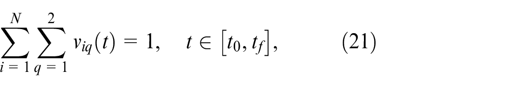
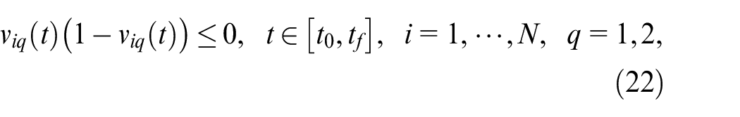
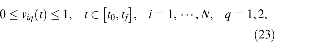
In this subsection, some auxiliary piecewise-constant functions $v_{\mathrm{iq}}\left(t\right):[t_0,t_f]\to [0,1]$ , $i=1,\cdots ,N$ , $q=1,2$ , are introduced for each subsystem, and these auxiliary functions satisfy the following continuous-time inequality constraints:

$$\sum _{i=1}^N\sum _{q=1}^2{v}_{\mathrm{iq}}\left(t\right)=1,t\in [t_0,t_f],$$

(21)

$$v_{\mathrm{iq}}\left(t\right)(1-v_{\mathrm{iq}}\left(t\right))\le 0,t\in [t_0,t_f],i=1,\cdots ,N,q=1,2,$$

(22)

$$0\le v_{\mathrm{iq}}\left(t\right)\le 1,t\in [t_0,t_f],i=1,\cdots ,N,q=1,2,$$

(23)

which ensure that for any $t\in [t_0,t_f]$ , there is one and only one pair $(i,q)$ such that $v_{\mathrm{iq}}=1$ and $v_{i\prime q\prime }=0$ for all $(i\prime ,q\prime )\ne (i,q)$ , where $i\in \{1,\cdots ,N\}$ and $q\in Q=\{1,2\}$ . Let $v(t)={[{\left(v_1\left(t\right)\right)}^{\mathrm{T}},\cdots ,{\left(v_N\left(t\right)\right)}^{\mathrm{T}}]}^{\mathrm{T}}$ , where $v_i\left(t\right)={[v_{i1}\left(t\right),v_{i2}\left(t\right)]}^{\mathrm{T}}$ , $i\in \{1,\cdots ,N\}$ . Then, Problem 2 is written as:

• Problem 3. Given the switched system

$$\stackrel{·}{\overline{x}}\left(t\right)=\sum _{i=1}^N\sum _{q=1}^2{v}_{\mathrm{iq}}(t)f_q(\overline{x}\left(t\right),{\sigma }^i){\chi }_{[{\tau }_{i-1},{\tau }_i)}\left(t\right),$$

(24)

with (10), choose a pair $(v(t),\sigma )\in (V,\mathrm{\Omega })$ such that

$$\hat{J}(v(t),\sigma )=-\sum _{i=1}^N{\int }_{{\tau }_{i-1}}^{{\tau }_i}{\overline{x}}_3\left(t\right)\mathrm{dt},$$

(25)

is minimized subject to the constraints (11), (17), (18), and (21)–(23).

Parameter optimization problem

In this section, the time-scaling transformation is used to obtain a more easily handled problem.

Time–scaling transformation

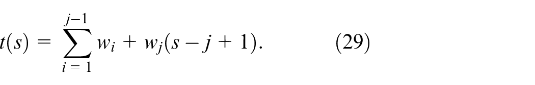
Let $\mathrm{t}\left(s\right):[0,N]\to R$ . Then, a time-scaling transformation is given by

$$\stackrel{·}{\mathrm{t}}\left(s\right)=\sum _{i=1}^N{w}_i{\chi }_{[i-1,i)}\left(s\right),$$

(26)

$$\mathrm{t}\left(0\right)=t_0,$$

(27)

where $w_i$ is the duration time of the $i\mathrm{th}$ switching, $s$ is a new time variable, and

$$t_0\le w_i={\tau }_i-{\tau }_{i-1}\le t_f,i=1,\cdots ,N.$$

(28)

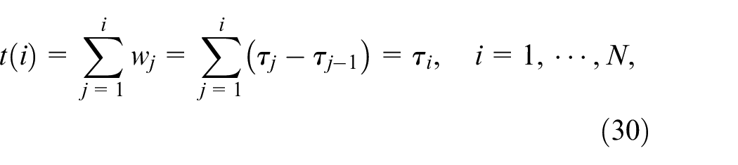
Let $w={[w_1,\cdots ,w_N]}^{\mathrm{T}}$ . Suppose that $W$ is the set consisting of all such $w$ . For any $s\in [j-1,j)$ , $j=1,\cdots ,N$ , from the ordinary differential equation described by (26) and (27), it follows that

$$t\left(s\right)=\sum _{i=1}^{j-1}{w}_i+w_j(s-j+1).$$

(29)

By using (29), we have

$$t\left(i\right)=\sum _{j=1}^i{w}_j=\sum _{j=1}^i({\tau }_j-{\tau }_{j-1})={\tau }_i,i=1,\cdots ,N,$$

(30)

$$t\left(N\right)=\sum _{j=1}^N{w}_j={\tau }_N=t_f.$$

(31)

Parameter optimization problem

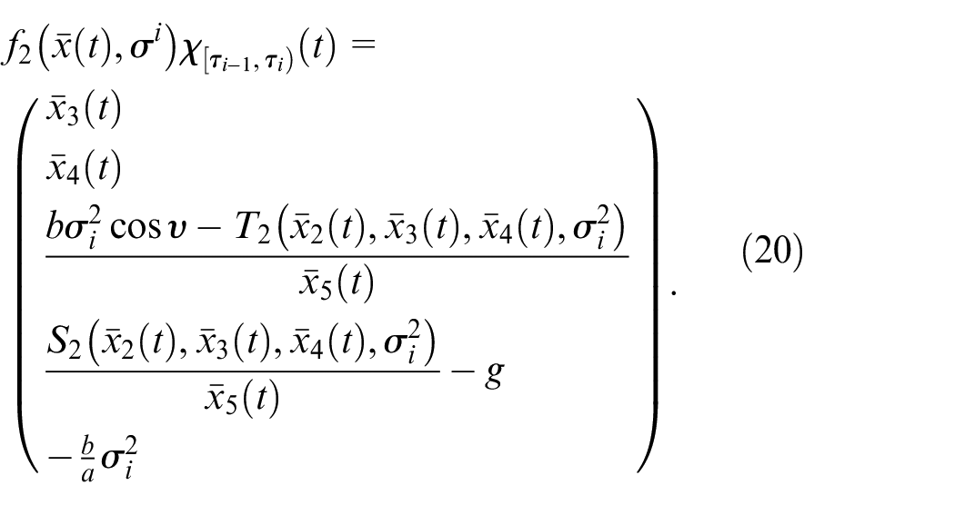
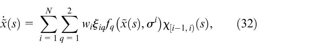
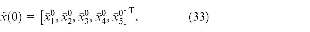
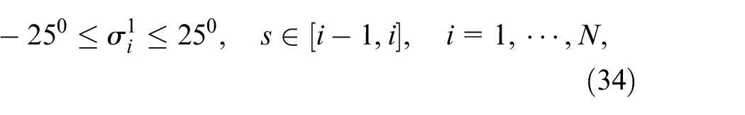
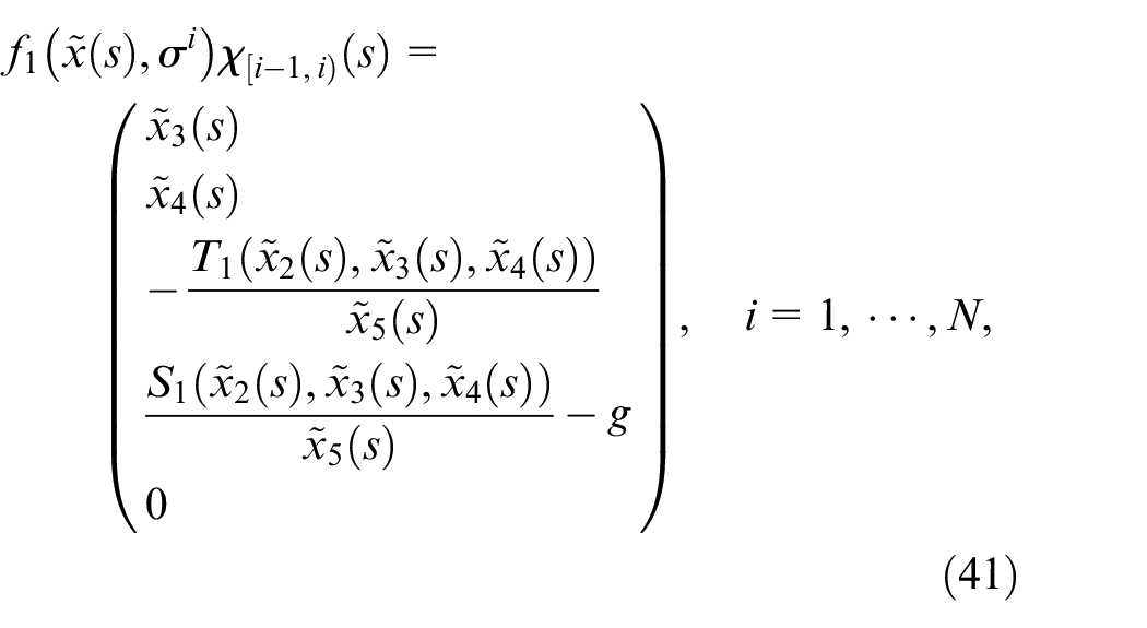
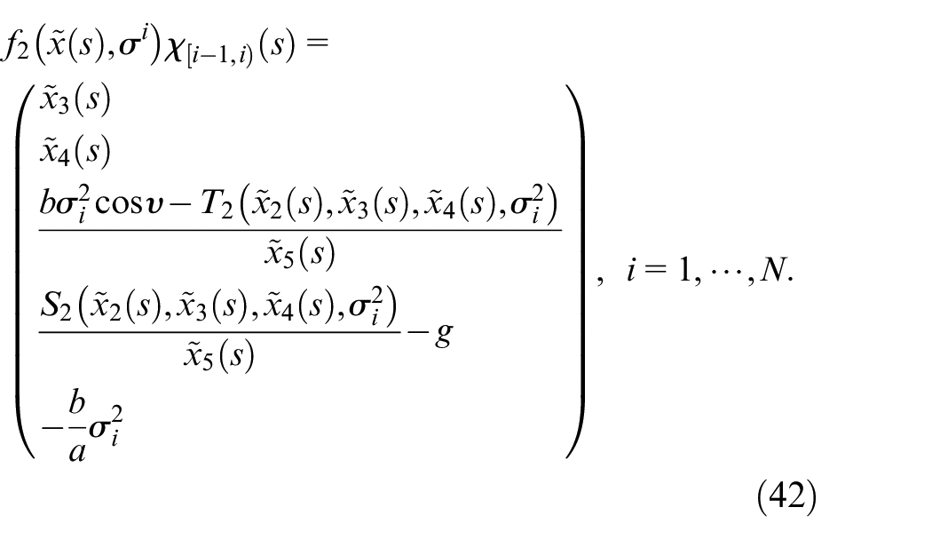
Suppose that ${\xi }_{\mathrm{iq}}$ is the value of $v_{\mathrm{iq}}\left(t\right)$ on $[{\tau }_{i-1},{\tau }_i)$ , where $i=1,\cdots ,N$ and $q=1,2$ . Define ${\xi }_i={[{\xi }_{i1},{\xi }_{i2}]}^{\mathrm{T}}\in R^2$ , $\xi ={[{\xi }_1^{\mathrm{T}},\cdots ,{\xi }_N^{\mathrm{T}}]}^{\mathrm{T}}\in R^{2N}$ , and suppose that $\Theta$ is the set consisting of all $\xi$ . Then, by applying (4.1) and (4.2) to the switched system (24) with (10), the constraints (17), (18), (21)–(23), (11), and the cost function (25), we obtain

$$\stackrel{·}{\stackrel{~}{x}}\left(s\right)=\sum _{i=1}^N\sum _{q=1}^2{w}_i{\xi }_{\mathrm{iq}}{f}_q(\tilde{x}\left(s\right),{\sigma }^i){\chi }_{[i-1,i)}\left(s\right),$$

(32)

$$\tilde{x}\left(0\right)={[{\overline{x}}_1^0,{\overline{x}}_2^0,{\overline{x}}_3^0,{\overline{x}}_4^0,{\overline{x}}_5^0]}^{\mathrm{T}},$$

(33)

$$-{25}^0\le {\sigma }_i^1\le {25}^0,s\in [i-1,i],i=1,\cdots ,N,$$

(34)

$$0\le {\sigma }_i^2\le 1,s\in [i-1,i],i=1,\cdots ,N,$$

(35)

$$\sum _{i=1}^N\sum _{q=1}^2{\xi }_{\mathrm{iq}}=1,s\in [0,N],$$

(36)

$${\xi }_{\mathrm{iq}}(1-{\xi }_{\mathrm{iq}})\le 0,s\in [0,N],i=1,\cdots ,N,q=1,2,$$

(37)

$$0\le {\xi }_{\mathrm{iq}}\le 1,s\in [0,N],i=1,\cdots ,N,q=1,2,$$

(38)

$$\tilde{x}\left(N\right)={\overline{x}}_{t_f},$$

(39)

$$\tilde{J}(\xi ,\sigma ,w)=-\sum _{i=1}^N{\int }_{i-1}^i{w}_i{\tilde{x}}_3\left(s\right)\mathrm{ds},$$

(40)

where ${\tilde{x}}_1\left(s\right)={\tilde{x}}_1\left(t\left(s\right)\right)$ , ${\tilde{x}}_2\left(s\right)={\tilde{x}}_2\left(t\left(s\right)\right)$ , ${\tilde{x}}_3\left(s\right)={\tilde{x}}_3\left(t\left(s\right)\right)$ , ${\tilde{x}}_4\left(s\right)={\tilde{x}}_4\left(t\left(s\right)\right)$ , ${\tilde{x}}_5\left(s\right)={\tilde{x}}_5\left(t\left(s\right)\right)$ , $\tilde{x}\left(s\right)={[{\tilde{x}}_1\left(s\right),{\tilde{x}}_2\left(s\right),{\tilde{x}}_3\left(s\right),{\tilde{x}}_4\left(s\right),{\tilde{x}}_5\left(s\right)]}^{\mathrm{T}}$ ; $w={[w_1,\cdots ,w_N]}^{\mathrm{T}}$ ;

$$\begin{array}{c}{f}_1(\tilde{x}\left(s\right),{\sigma }^i){\chi }_{[i-1,i)}\left(s\right)=\hfill \\ \left(\begin{array}{c}{\tilde{x}}_3\left(s\right)\hfill \\ \multicolumn{1}{c}{{\tilde{x}}_4\left(s\right)}\\ \multicolumn{1}{c}{-\frac{T_1({\tilde{x}}_2\left(s\right),{\tilde{x}}_3\left(s\right),{\tilde{x}}_4\left(s\right))}{{\tilde{x}}_5\left(s\right)}}\\ \multicolumn{1}{c}{\frac{S_1({\tilde{x}}_2\left(s\right),{\tilde{x}}_3\left(s\right),{\tilde{x}}_4\left(s\right))}{{\tilde{x}}_5\left(s\right)}-g}\\ \multicolumn{1}{c}{0}\end{array}\right),i=1,\cdots ,N,\hfill \end{array}$$

(41)

and

$$\begin{array}{c}{f}_2(\tilde{x}\left(s\right),{\sigma }^i){\chi }_{[i-1,i)}\left(s\right)=\hfill \\ \left(\begin{array}{c}{\tilde{x}}_3\left(s\right)\hfill \\ \multicolumn{1}{c}{{\tilde{x}}_4\left(s\right)}\\ \multicolumn{1}{c}{\frac{b{\sigma }_i^2\cos \upsilon -T_2({\tilde{x}}_2\left(s\right),{\tilde{x}}_3\left(s\right),{\tilde{x}}_4\left(s\right),{\sigma }_i^2)}{{\tilde{x}}_5\left(s\right)}}\\ \multicolumn{1}{c}{\frac{S_2({\tilde{x}}_2\left(s\right),{\tilde{x}}_3\left(s\right),{\tilde{x}}_4\left(s\right),{\sigma }_i^2)}{{\tilde{x}}_5\left(s\right)}-g}\\ \multicolumn{1}{c}{-\frac{b}{a}{\sigma }_i^2}\end{array}\right),i=1,\cdots ,N.\hfill \end{array}$$

(42)

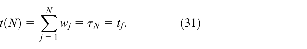
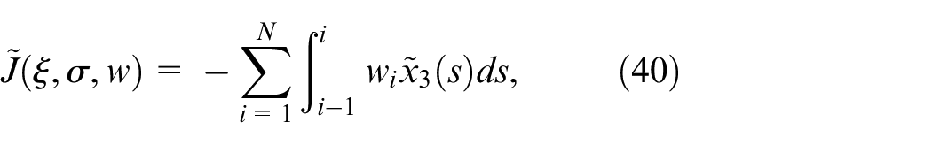
Let $W$ be set containing all $w$ . Problem 3 becomes an equivalent parameter optimization problem as follows.

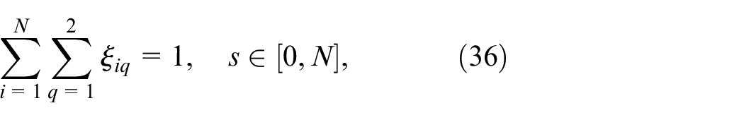
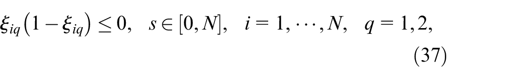
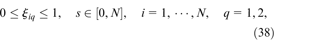
• Problem 4. Given the switched system (32) with (10), find a triple $(\xi ,\sigma ,w)\in (\Theta ,\mathrm{\Omega },W)$ such that the cost function (40) is minimized subject to the constraints (31), (34), (35), (36)–(38), and (39).

A penalty function-based improved CFF algorithm

In this section, a penalty function-based improved CFF algorithm is developed for solving the parameter optimization problem described by Section 4.

A penalty optimization problem

Since the inequality constraints (36)–(38) define a non-connected feasible region for ${\xi }_{\mathrm{iq}}$ , $i=1,\cdots ,N$ , $q=1,2$ , it is challenging to find a solution of Problem 4. To avoid this challenging, we can define a penalty optimization problem by using the idea in^33–35:

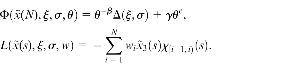
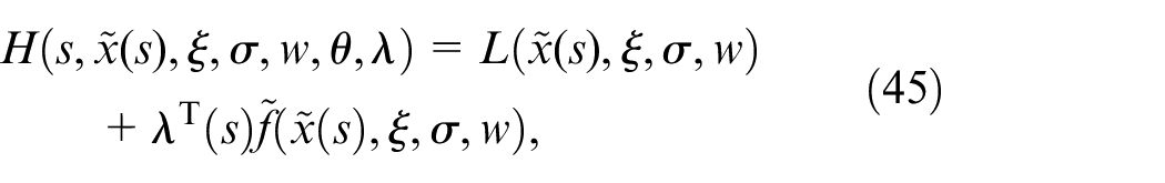
• Problem 5. Given the switched system (32) with (10), find a tetrad $(\xi ,\sigma ,w,\theta )\in (\Theta ,\mathrm{\Omega },W,\Lambda )$ such that

$${\tilde{J}}_{\gamma }(\xi ,\sigma ,w,\theta )=\tilde{J}(\xi ,\sigma ,w)+{\theta }^{-\beta }\mathrm{\Delta }(\xi ,\sigma )+\gamma {\theta }^c,$$

(43)

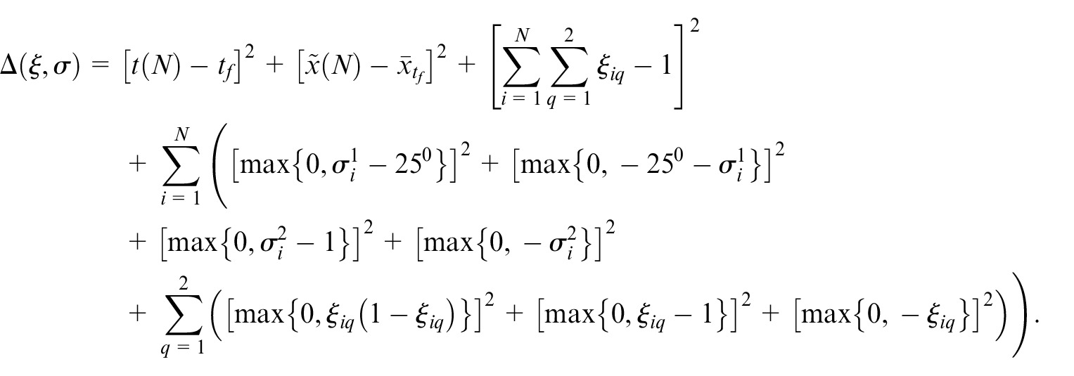
is minimized, where $\gamma >0$ and $\theta >0$ denote a penalty parameter variable and a new decision variable, respectively; $\beta$ and $c$ are given positive real numbers satisfying $\beta >c>1$ ; $\Lambda$ denotes the set containing all such $\theta$ ; $\mathrm{\Delta }(\xi ,\sigma )$ is the constraint’s violation; and $\mathrm{\Delta }(\xi ,\sigma )$ is defined by

$$\begin{array}{l}\mathrm{\Delta }\left(\xi ,\sigma \right)={\left[t\left(N\right)-t_f\right]}^2+{\left[\tilde{x}\left(N\right)-{\overline{x}}_{t_f}\right]}^2+{\left[\sum _{i=1}^N\sum _{q=1}^2{\xi }_{iq}-1\right]}^2\\ +\sum _{i=1}^N({\left[\max \left\{0,{\sigma }_i^1-{25}^0\right\}\right]}^2+{\left[\max \left\{0,-{25}^0-{\sigma }_i^1\right\}\right]}^2+{\left[\max \left\{0,{\sigma }_i^2-1\right\}\right]}^2\\ +{\left[\max \left\{0,-{\sigma }_i^2\right\}\right]}^2+\sum _{q=1}^2\left({\left[\max \left\{0,{\xi }_{iq}\left(1-{\xi }_{iq}\right)\right\}\right]}^2+{\left[\max \left\{0,{\xi }_{iq}-1\right\}\right]}^2+{\left[\max \left\{0,-{\xi }_{iq}\right\}\right]}^2\right)).\end{array}$$

• Remark 1. Note that the positive real number $c$ is given. Then, during the minimizing process of ${\tilde{J}}_{\gamma }(\xi ,\sigma ,w,\theta )$ , if $\gamma$ is increased, ${\theta }^c$ should be reduced, which indicates that the decision variable $\theta$ should be reduced. Thus, ${\theta }^{-\beta }$ will be increased and $\mathrm{\Delta }(\xi ,\sigma )$ will be reduced, which indicates that any solution of Problem 5 satisfies Problem 4, as $\gamma \to +\infty$ .

Gradient formulas

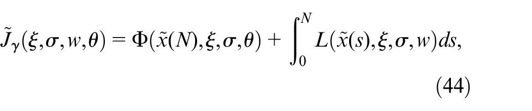
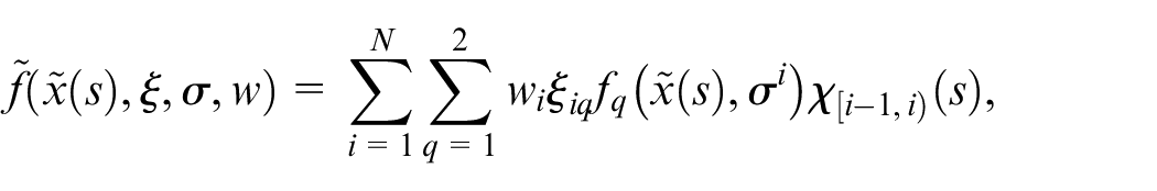
Firstly, the cost function (43) can be written as follows:

$${\tilde{J}}_{\gamma }(\xi ,\sigma ,w,\theta )=\mathrm{\Phi }(\tilde{x}(N),\xi ,\sigma ,\theta )+{\int }_0^{N}L(\tilde{x}(s),\xi ,\sigma ,w)\mathrm{ds},$$

(44)

where

$$\begin{array}{c}\mathrm{\Phi }(\tilde{x}(N),\xi ,\sigma ,\theta )={\theta }^{-\beta }\mathrm{\Delta }(\xi ,\sigma )+\gamma {\theta }^c,\hfill \\ L(\tilde{x}(s),\xi ,\sigma ,w)=-\sum _{i=1}^N{w}_i{\tilde{x}}_3\left(s\right){\chi }_{[i-1,i)}\left(s\right).\hfill \end{array}$$

Then, we can define the Hamiltonian function $H(s,\tilde{x}(s),\xi ,\sigma ,w,\theta ,\lambda )$ by

$$\begin{array}{c}H(s,\tilde{x}(s),\xi ,\sigma ,w,\theta ,\lambda )=L(\tilde{x}(s),\xi ,\sigma ,w)\hfill \\ +{\lambda }^{\mathrm{T}}\left(s\right)\tilde{f}(\tilde{x}\left(s\right),\xi ,\sigma ,w),\hfill \end{array}$$

(45)

where

$$\tilde{f}(\tilde{x}\left(s\right),\xi ,\sigma ,w)=\sum _{i=1}^N\sum _{q=1}^2{w}_i{\xi }_{\mathrm{iq}}{f}_q(\tilde{x}\left(s\right),{\sigma }^i){\chi }_{[i-1,i)}\left(s\right),$$

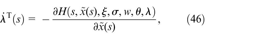
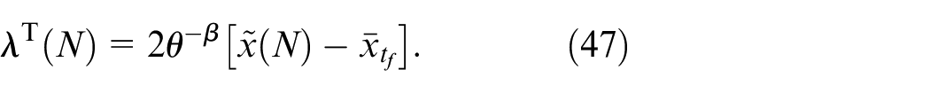
and the costate $\lambda \left(s\right)$ satisfies

$${\stackrel{·}{\lambda }}^{\mathrm{T}}\left(s\right)=-\frac{\partial H(s,\tilde{x}(s),\xi ,\sigma ,w,\theta ,\lambda )}{\partial \tilde{x}(s)},$$

(46)

with

$${\lambda }^{\mathrm{T}}\left(N\right)=2{\theta }^{-\beta }[\tilde{x}\left(N\right)-{\overline{x}}_{t_f}].$$

(47)

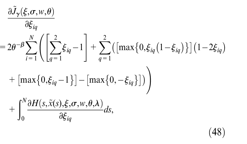
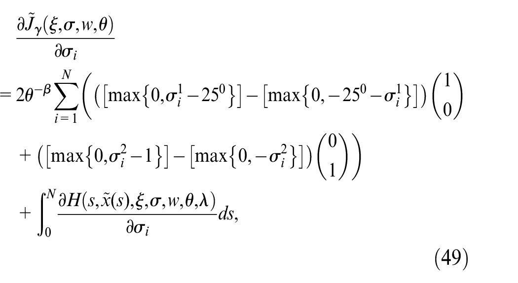
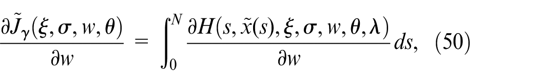
• Theorem 1. For $i\in \{1,\cdots ,N\}$ and $q\in \{1,2\}$ , the gradient of the function (44) with the variables ${\xi }_{\mathrm{iq}}$ , ${\sigma }_i$ , $w$ , and $\theta$ are expressed by

$$\begin{array}{c}\frac{\partial {\tilde{J}}_{\gamma }(\xi ,\sigma ,w,\theta )}{\partial {\xi }_{\mathrm{iq}}}\hfill \\ \multicolumn{1}{c}{=2{\theta }^{-\beta }\sum _{i=1}^N([\sum _{q=1}^2{\xi }_{\mathrm{iq}}-1]+\sum _{q=1}^2([max\{0,{\xi }_{\mathrm{iq}}(1-{\xi }_{\mathrm{iq}})\}](1-2{\xi }_{\mathrm{iq}})}\\ +[max\{0,{\xi }_{\mathrm{iq}}-1\}]-[max\{0,-{\xi }_{\mathrm{iq}}\}]))\hfill \\ +{\int }_0^N\frac{\partial H(s,\tilde{x}(s),\xi ,\sigma ,w,\theta ,\lambda )}{\partial {\xi }_{\mathrm{iq}}}\mathrm{ds},\hfill \end{array}$$

(48)

$$\begin{array}{c}\frac{\partial {\tilde{J}}_{\gamma }(\xi ,\sigma ,w,\theta )}{\partial {\sigma }_i}\hfill \\ \multicolumn{1}{c}{=2{\theta }^{-\beta }\sum _{i=1}^N(([max\{0,{\sigma }_i^1-{25}^0\}]-[max\{0,-{25}^0-{\sigma }_i^1\}])\left(\begin{array}{c}1\hfill \\ \multicolumn{1}{c}{0}\end{array}\right)}\\ +([max\{0,{\sigma }_i^2-1\}]-[max\{0,-{\sigma }_i^2\}])\left(\begin{array}{c}0\hfill \\ \multicolumn{1}{c}{1}\end{array}\right))\hfill \\ +{\int }_0^N\frac{\partial H(s,\tilde{x}(s),\xi ,\sigma ,w,\theta ,\lambda )}{\partial {\sigma }_i}\mathrm{ds},\hfill \end{array}$$

(49)

$$\frac{\partial {\tilde{J}}_{\gamma }(\xi ,\sigma ,w,\theta )}{\partial w}={\int }_0^N\frac{\partial H(s,\tilde{x}(s),\xi ,\sigma ,w,\theta ,\lambda )}{\partial w}\mathrm{ds},$$

(50)

$$\begin{array}{c}\frac{\partial {\tilde{J}}_{\gamma }(\xi ,\sigma ,w,\theta )}{\partial \theta }\hfill \\ =c\gamma {\theta }^{c-1}-\beta {\theta }^{-\beta -1}\mathrm{\Delta }(\xi ,\sigma )+{\int }_0^N\frac{\partial H(s,\tilde{x}(s),\xi ,\sigma ,w,\theta ,\lambda )}{\partial \theta }\mathrm{ds}.\hfill \end{array}$$

(51)

Proof. Applying (32) and (45) to (44) yields

$$\begin{array}{c}{\tilde{J}}_{\gamma }(\xi ,\sigma ,w,\theta )=\mathrm{\Phi }(\tilde{x}(N),\xi ,\sigma ,\theta )\hfill \\ +{\int }_0^N(H(s,\tilde{x}(s),\xi ,\sigma ,w,\theta ,\lambda )-{\lambda }^{\mathrm{T}}\left(s\right)\stackrel{·}{\stackrel{~}{x}}\left(s\right))\mathrm{ds}\hfill \\ =\mathrm{\Phi }(\tilde{x}(N),\xi ,\sigma ,\theta )-{\lambda }^{\mathrm{T}}\left(N\right)\tilde{x}\left(N\right)+{\lambda }^{\mathrm{T}}\left(0\right)\tilde{x}\left(0\right)\hfill \\ +{\int }_0^N(H(s,\tilde{x}(s),\xi ,\sigma ,w,\theta ,\lambda )+{\stackrel{·}{\lambda }}^{\mathrm{T}}\left(s\right)\tilde{x}\left(s\right))\mathrm{ds}.\hfill \end{array}$$

(52)

Then, the first order variation of (52) is presented as follows:

$$\begin{array}{c}\delta {\tilde{J}}_{\gamma }(\xi ,\sigma ,w,\theta )\hfill \\ =2{\theta }^{-\beta }\sum _{i=1}^N((([max\{0,{\sigma }_i^1-{25}^0\}]-[max\{0,-{25}^0-{\sigma }_i^1\}])\left(\begin{array}{c}1\hfill \\ \multicolumn{1}{c}{0}\end{array}\right)\hfill \\ +([max\{0,{\sigma }_i^2-1\}]-[max\{0,-{\sigma }_i^2\}])\left(\begin{array}{c}0\hfill \\ \multicolumn{1}{c}{1}\end{array}\right))\delta {\sigma }_i\hfill \\ +([\sum _{q=1}^2{\xi }_{\mathrm{iq}}-1]+\sum _{q=1}^2([max\{0,{\xi }_{\mathrm{iq}}(1-{\xi }_{\mathrm{iq}})\}](1-2{\xi }_{\mathrm{iq}})\hfill \\ +[max\{0,{\xi }_{\mathrm{iq}}-1\}]-[max\{0,-{\xi }_{\mathrm{iq}}\}])\delta {\xi }_{\mathrm{iq}})))\hfill \\ +(2{\theta }^{-\beta }[\tilde{x}\left(N\right)-{\overline{x}}_{t_f}]-{\lambda }^{\mathrm{T}}\left(N\right))\delta \tilde{x}\left(N\right)\hfill \\ +(c\gamma {\theta }^{c-1}-\beta {\theta }^{-\beta -1}\mathrm{\Delta }(\xi ,\sigma ))\delta \theta +{\lambda }^{\mathrm{T}}\left(0\right)\delta \tilde{x}\left(0\right)\hfill \\ +{\int }_0^N(\frac{\partial H(s,\tilde{x}(s),\xi ,\sigma ,w,\theta ,\lambda )}{\partial \tilde{x}(s)}\delta \tilde{x}(s)+\frac{\partial H(s,\tilde{x}(s),\xi ,\sigma ,w,\theta ,\lambda )}{\partial {\xi }_{\mathrm{iq}}}\delta {\xi }_{\mathrm{iq}}\hfill \\ +\frac{\partial H(s,\tilde{x}(s),\xi ,\sigma ,w,\theta ,\lambda )}{\partial {\sigma }_i}\delta {\sigma }_i+\frac{\partial H(s,\tilde{x}(s),\xi ,\sigma ,w,\theta ,\lambda )}{\partial w}\delta w\hfill \\ +{\stackrel{·}{\lambda }}^{\mathrm{T}}\left(s\right)\delta \tilde{x}\left(s\right))\mathrm{ds}.\hfill \end{array}$$

(53)

Applying (46) and (47) to (53) gives

$$\begin{array}{c}\delta {\tilde{J}}_{\gamma }(\xi ,\sigma ,w,\theta )\hfill \\ \multicolumn{1}{c}{=2{\theta }^{-\beta }\sum _{i=1}^N((([max\{0,{\sigma }_i^1-{25}^0\}]-[max\{0,-{25}^0-{\sigma }_i^1\}])\left(\begin{array}{c}1\hfill \\ \multicolumn{1}{c}{0}\end{array}\right)}\\ +([max\{0,{\sigma }_i^2-1\}]-[max\{0,-{\sigma }_i^2\}])\left(\begin{array}{c}0\hfill \\ \multicolumn{1}{c}{1}\end{array}\right))\delta {\sigma }_i\hfill \\ +([\sum _{q=1}^2{\xi }_{\mathrm{iq}}-1]+\sum _{q=1}^2([max\{0,{\xi }_{\mathrm{iq}}(1-{\xi }_{\mathrm{iq}})\}](1-2{\xi }_{\mathrm{iq}})\hfill \\ +[max\{0,{\xi }_{\mathrm{iq}}-1\}]-[max\{0,-{\xi }_{\mathrm{iq}}\}])\delta {\xi }_{\mathrm{iq}})))\hfill \\ +{\int }_0^N(\frac{\partial H(s,\tilde{x}(s),\xi ,\sigma ,w,\theta ,\lambda )}{\partial {\xi }_{\mathrm{iq}}}\delta {\xi }_{\mathrm{iq}}+\frac{\partial H(s,\tilde{x}(s),\xi ,\sigma ,w,\theta ,\lambda )}{\partial {\sigma }_i}\delta {\sigma }_i\hfill \\ +\frac{\partial H(s,\tilde{x}(s),\xi ,\sigma ,w,\theta ,\lambda )}{\partial w}\delta w)\mathrm{ds}+(c\gamma {\theta }^{c-1}-\beta {\theta }^{-\beta -1}\mathrm{\Delta }(\xi ,\sigma ))\delta \theta .\hfill \end{array}$$

(54)

Thus, the gradient formulas (48)–(51) of (44) can be obtained by using (54). ■

An improved continuous filled function

In order to avoid the shortcomings of the existing CFF, an improved CFF with an adjusting parameter is develop in this subsection. The improved CFF is differentiable and excludes exponential terms or logarithmic terms. More importantly, any one local solution of the improved CFF is a better local solution of the original parameter optimization problem.

Let $\rho ={[{\xi }^{\mathrm{T}},{\sigma }^{\mathrm{T}},w^{\mathrm{T}},\theta ]}^{\mathrm{T}}$ . Suppose that $\mathrm{\Upsilon }$ is the set consisting of all such $\rho$ . Following that, an improved CFF is defined as follows:

• Definition 1. It is assumed that ${\rho }^{*}$ denotes a local minimizer of ${\tilde{J}}_{\gamma }\left(\rho \right)$ . Then, $\tilde{F}\left(\rho \right)$ is called a CFF of ${\tilde{J}}_{\gamma }\left(\rho \right)$ at the local minimizer ${\rho }^{*}$ , if $\tilde{F}\left(\rho \right)$ own three properties:

• (1)  ${\rho }^{*}$ is also a strict local maximizer of the function $\tilde{F}\left(\rho \right)$ ;

• (2) For any $\rho \in E_1$ , $\nabla \tilde{F}\left(\rho \right)\ne 0$ , where ∇ denotes the gradient operator and $E_1$ is a set defined by

$$E_1=\{\rho |{\tilde{J}}_{\gamma }\left(\rho \right)\ge {\tilde{J}}_{\gamma }\left({\rho }^{*}\right),\rho \in \mathrm{\Upsilon }\backslash \left\{{\rho }^{*}\right\}\};$$

• (3) If ${\rho }^{*}$ is not a global minimizer of ${\tilde{J}}_{\gamma }\left(\rho \right)$ , then a local minimizer $\rho \prime$ of $\tilde{F}\left(\rho \right)$ can be obtained on the set $E_2$ , where

$$E_2=\{\rho |{\tilde{J}}_{\gamma }\left(\rho \right)<{\tilde{J}}_{\gamma }\left({\rho }^{*}\right),\rho \in \mathrm{\Upsilon }\}.$$

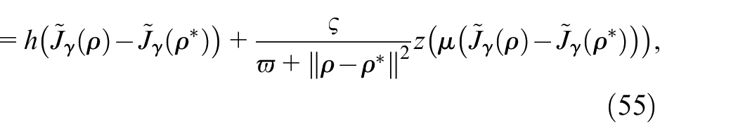
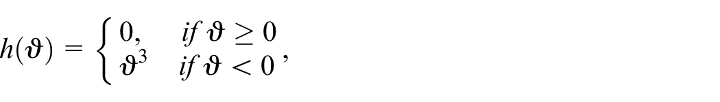
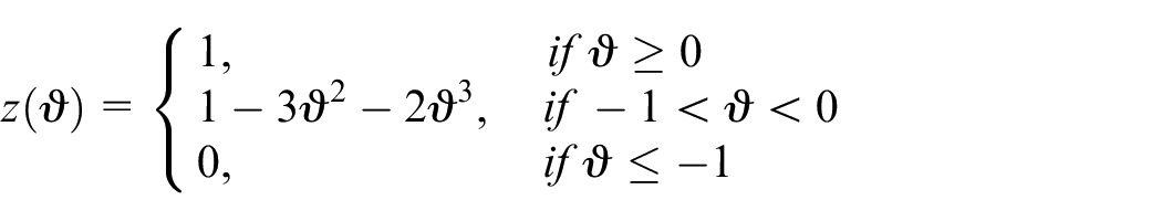
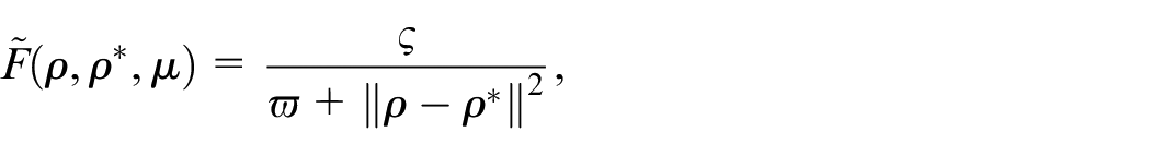
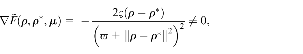
Now, at the local minimizer ${\rho }^{*}$ , an improved CFF can be constructed for solving Problem 5 as follows:

$$\tilde{F}(\rho ,{\rho }^{*},\mu )$$

$$=h({\tilde{J}}_{\gamma }\left(\rho \right)-{\tilde{J}}_{\gamma }\left({\rho }^{*}\right))+\frac{\varsigma }{\varpi +{\Vert \rho -{\rho }^{*}\Vert }^2}z\left(\mu ({\tilde{J}}_{\gamma }\left(\rho \right)-{\tilde{J}}_{\gamma }\left({\rho }^{*}\right))\right),$$

(55)

where the functions $h$ and $z$ are, respectively, defined by

$$h\left(\vartheta \right)=\{\begin{array}{cc}0,\hfill & \mathrm{if}\vartheta \ge 0\hfill \\ \multicolumn{1}{c}{{\vartheta }^3}& \mathrm{if}\vartheta <0\hfill \end{array},$$

$$z\left(\vartheta \right)=\{\begin{array}{cc}1,\hfill & \mathrm{if}\vartheta \ge 0\hfill \\ \multicolumn{1}{c}{1-3{\vartheta }^2-2{\vartheta }^3,}& \mathrm{if}-1<\vartheta <0\hfill \\ \multicolumn{1}{c}{0,}& \mathrm{if}\vartheta \le -1\hfill \end{array}$$

$\varsigma$ , $\varpi$ , and $\mu$ are positive real numbers.

Then, the following theorem will show that the function (55) is a CFF satisfying the properties of Definition 1.

• Theorem 2. Let ${\rho }^{*}$ be a local minimizer of ${\tilde{J}}_{\gamma }\left(\rho \right)$ and the function $\tilde{F}(\rho ,{\rho }^{*},\mu )$ be defined by (55). Then, for any $\mu >0$ , ${\rho }^{*}$ is a strict local maximizer of $\tilde{F}(\rho ,{\rho }^{*},\mu )$ on $\mathrm{\Upsilon }$ .

Proof. Note that ${\rho }^{*}$ is a local minimizer of ${\tilde{J}}_{\gamma }\left(\rho \right)$ . Then, for any $\rho \in \mathrm{\Upsilon }\cap N({\rho }^{*},\epsilon )$ , there is a $\epsilon >0$ such that ${\tilde{J}}_{\gamma }\left(\rho \right)\ge {\tilde{J}}_{\gamma }\left({\rho }^{*}\right)$ , where $N({\rho }^{*},\epsilon )$ is a $\epsilon$ neighborhood of ${\rho }^{*}$ defined by

$$N({\rho }^{*},\epsilon )=\{\rho |\Vert \rho -{\rho }^{*}\Vert <\epsilon \}.$$

Thus, for any $\rho \in \mathrm{\Upsilon }\cap N({\rho }^{*},\epsilon )$ and $\rho \ne {\rho }^{*}$ , we obtain

$$\tilde{F}(\rho ,{\rho }^{*},\mu )=\frac{\varsigma }{\varpi +{\Vert \rho -{\rho }^{*}\Vert }^2}<\frac{\varsigma }{\varpi }=\tilde{F}({\rho }^{*},{\rho }^{*},\mu ),$$

which shows that for any $\mu >0$ , ${\rho }^{*}$ is a strict local maximizer of $\tilde{F}(\rho ,{\rho }^{*},\mu )$ on $\mathrm{\Upsilon }$ . ■

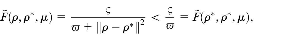
• Theorem 3. Suppose that ${\rho }^{*}$ is a local minimizer of ${\tilde{J}}_{\gamma }\left(\rho \right)$ . Then, for any $\rho \in E_1$ and the positive real number $\mu$ , we have $\nabla \tilde{F}(\rho ,{\rho }^{*},\mu )\ne 0$ .

Proof. Note that $\rho \in E_1$ . Then, by using the function described by (55), we obtain $\rho \ne {\rho }^{*}$ ,

$$\tilde{F}(\rho ,{\rho }^{*},\mu )=\frac{\varsigma }{\varpi +{\Vert \rho -{\rho }^{*}\Vert }^2},$$

and

$$\nabla \tilde{F}(\rho ,{\rho }^{*},\mu )=-\frac{2\varsigma (\rho -{\rho }^{*})}{{(\varpi +{\Vert \rho -{\rho }^{*}\Vert }^2)}^2}\ne 0,$$

for any $\rho \in E_1$ and the positive real number $\mu$ . ■

To illustrate the function $\tilde{F}(\rho ,{\rho }^{*},\mu )$ satisfying the $3$ rd property of Definition 1, it is assumed that ${\tilde{J}}_{\gamma }\left(\rho \right)$ satisfies the following two assumptions.

• Assumption 1. Suppose that ${\tilde{J}}_{\gamma }\left(\rho \right)$ has only a finite number of minimizers in $\mathrm{\Upsilon }$ and the set consisting of the minimizers is defined by

$$\mathrm{\Pi }=\{{\rho }_i^{*}|i=1,\cdots ,M\}.$$

Here, $M$ denotes the number of minimizer of ${\tilde{J}}_{\gamma }\left(\rho \right)$ .

• Assumption 2. Suppose that all of the local minimizers of ${\tilde{J}}_{\gamma }\left(\rho \right)$ fall into the interior of $\mathrm{\Upsilon }$ , and any point $\rho$ on the boundary of $\mathrm{\Upsilon }$ satisfies ${\tilde{J}}_{\gamma }\left(\rho \right)>d$ , where

$$d=max\{{\tilde{J}}_{\gamma }\left(\rho \right)|\rho \in \mathrm{\Pi }\}.$$

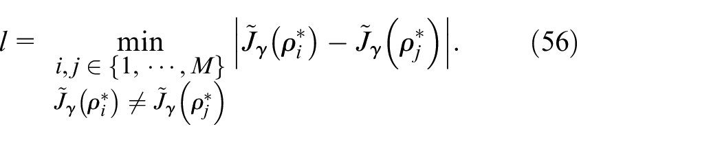
• Theorem 4. Let ${\rho }^{*}$ be a local minimizer but not a global minimizer of ${\tilde{J}}_{\gamma }\left(\rho \right)$ on $\mathrm{\Upsilon }$ , which implies that the set $E_2$ is not empty. Then, there is a $\rho \prime \in E_2$ such that $\rho \prime$ is a local minimizer of the function $\tilde{F}(\rho ,{\rho }^{*},\mu )$ , as $\mu >\frac{1}{2l}$ , where $l$ is given by

$$l=\underset{\begin{array}{c}i,j\in \{1,\cdots ,M\}\hfill \\ \multicolumn{1}{c}{{\tilde{J}}_{\gamma }\left({\rho }_i^{*}\right)\ne {\tilde{J}}_{\gamma }\left({\rho }_j^{*}\right)}\end{array}}{min}|{\tilde{J}}_{\gamma }\left({\rho }_i^{*}\right)-{\tilde{J}}_{\gamma }\left({\rho }_j^{*}\right)|.$$

(56)

Proof. Note that ${\rho }^{*}$ is a local minimizer but not a global minimizer of ${\tilde{J}}_{\gamma }\left(\rho \right)$ on $\mathrm{\Upsilon }$ . Then, another local minimizer ${\tilde{\rho }}^{*}$ of ${\tilde{J}}_{\gamma }\left(\rho \right)$ can be obtained such that

$${\tilde{J}}_{\gamma }\left({\tilde{\rho }}^{*}\right)<{\tilde{J}}_{\gamma }\left({\rho }^{*}\right).$$

(57)

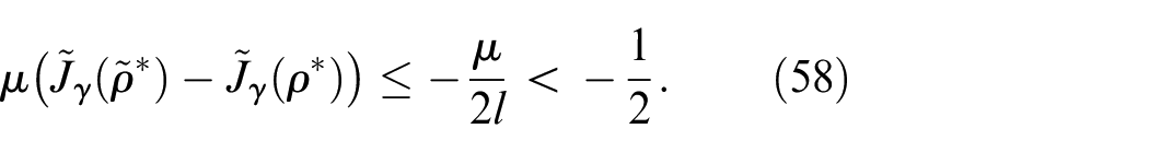
By using definition of $l$ described by (56) and the continuity of ${\tilde{J}}_{\gamma }\left(\rho \right)$ , as long as $\mu >\frac{1}{2l}$ , the following inequality can be obtain:

$$\mu ({\tilde{J}}_{\gamma }\left({\tilde{\rho }}^{*}\right)-{\tilde{J}}_{\gamma }\left({\rho }^{*}\right))\le -\frac{\mu }{2l}<-\frac{1}{2}.$$

(58)

Applying (57) and (58) to the function $\tilde{F}(\rho ,{\rho }^{*},\mu )$ described by (55) yields

$$\tilde{F}({\tilde{\rho }}^{*},{\rho }^{*},\mu )={({\tilde{J}}_{\gamma }\left({\tilde{\rho }}^{*}\right)-{\tilde{J}}_{\gamma }\left({\rho }^{*}\right))}^3<0.$$

(59)

By using Assumption 2, for any $\rho ″\in \partial \mathrm{\Upsilon }$ , we have

$${\tilde{J}}_{\gamma }(\rho ″)<{\tilde{J}}_{\gamma }\left({\rho }^{*}\right),$$

(60)

where $\partial \mathrm{\Upsilon }$ denotes the boundary of $\mathrm{\Upsilon }$ . Then, by applying (60) to the function $\tilde{F}(\rho ,{\rho }^{*},\mu )$ described by (55), we obtain

$$\tilde{F}(\rho ″,{\rho }^{*},\mu )=\frac{\varsigma }{\varpi +{\Vert \rho ″-{\rho }^{*}\Vert }^2}>0.$$

(61)

Since $\tilde{F}(\rho ,{\rho }^{*},\mu )$ defined by (55) is continuous, the inequalities (59) and (61) imply that there is a $\rho ″\prime$ on the line segment between $\rho ″$ and ${\tilde{\rho }}^{*}$ such that

$$\tilde{F}(\rho ″\prime ,{\rho }^{*},\mu )=0.$$

Thus, we obtain a line segment between $\rho ″\prime$ and ${\tilde{\rho }}^{*}$ . Suppose that $E\left({\tilde{\rho }}^{*}\right)$ is the set containing all such line segments. Clearly, the set $E\left({\tilde{\rho }}^{*}\right)$ is a closed region. By using continuity of $\tilde{F}(\rho ,{\rho }^{*},\mu )$ described by (55), there is a point $\rho \prime \in E\left({\tilde{\rho }}^{*}\right)\subset E_2$ which is a local minimizer of $\tilde{F}(\rho ,{\rho }^{*},\mu )$ . ■

A penalty function-based improved CFF algorithm

In this subsection, a penalty function-based improved CFF algorithm will be developed for obtaining a global optimal solution to Problem 1 based on Theorems 1–4 and above discussions.

• Algorithm 1. A penalty function-based improved CFF algorithm for solving Problem 1.

• Step 1: Set $\mu :=1$ , $\varsigma :=1$ , $\varpi :=1$ , $j:=1$ , $k:=1$ and choose ${\rho }_k\in \mathrm{\Upsilon }$ , the tolerance $\zeta >0$ , the upper bound $\tilde{\mu }$ of $\mu$ .

• Step 2: By using the steepest descent algorithm with Armijo step size, solve Problem 5 starting from the initial point ${\rho }_k\in \mathrm{\Upsilon }$ . If $\Vert \nabla {\tilde{J}}_{\gamma }\Vert \le \zeta$ , stop. Let ${\rho }_k^{*}:={\rho }_k$ be a local minimizer of Problem 5 and go to Step 3, where $\nabla {\tilde{J}}_{\gamma }$ denotes the gradient of ${\tilde{J}}_{\gamma }$ and ‖·‖ denotes the Euclidean norm.

• Step 3: Construct a continuous filled function as follows:

$$\begin{array}{c}\tilde{F}(\rho ,{\rho }_k^{*},\mu )\hfill \\ =h({\tilde{J}}_{\gamma }\left(\rho \right)-{\tilde{J}}_{\gamma }\left({\rho }_k^{*}\right))+\frac{\varsigma }{\varpi +{\Vert \rho -{\rho }_k^{*}\Vert }^2}z\left(\mu ({\tilde{J}}_{\gamma }\left(\rho \right)-{\tilde{J}}_{\gamma }\left({\rho }_k^{*}\right))\right).\hfill \end{array}$$

• Step 4: If $j\le 2K$ , then set $\rho :={\rho }_k^{*}+p{e}_j$ , go to step 5, otherwise, go to Step 6, where $K$ is the dimension of Problem 5; $e_j={\underset{j}{[0,\cdots ,1,\cdots ,0]}}^{\mathrm{T}}$ , $j=1,\cdots ,K$ , $e_j=-e_{j-K}$ , $j=K+1,\cdots ,2K$ .

• Step 5: By using the steepest descent algorithm with Armijo step size, minimize the continuous filled function $\tilde{F}(\rho ,{\rho }_k^{*},\mu )$ by using $\rho$ as an initial point. If the minimization sequences of the continuous filled function $\tilde{F}(\rho ,{\rho }_k^{*},\mu )$ go out of the set $\mathrm{\Upsilon }$ , set $j:=j+1$ and go to Step 4, otherwise, a minimizer $\rho \prime$ will be obtained by minimizing the CFF $\tilde{F}(\rho ,{\rho }_k^{*},\mu )$ , set ${\rho }_k^{*}:=\rho \prime$ , $k:=k+1$ , and go to Step 3.

• Step 6: If $\mu <\tilde{\mu }$ , then set $\mu :=10\mu$ and go to Step 3, otherwise, this algorithm stops and let ${\rho }_k^{*}$ be a global minimizer of Problem 5, and go to Step 7.

• Step 7: The solution of Problem 1 is constructed by using the global minimizer ${\rho }_k^{*}$ of Problem 5.

• Remark 2. In Step 4, the value of the parameter $p$ requires o be chosen precisely. In Algorithm 1, $p$ is chosen to ensure $\Vert \nabla \tilde{F}(\rho ,{\rho }_k^{*},\mu )\Vert$ is greater than a certain threshold, e.g. ${10}^{-3}$ ). Step 5 indicates that the local minimizer $\rho \prime$ of the CFF $\tilde{F}(\rho ,{\rho }_k^{*},\mu )$ satisfies $\rho \prime \in E_2$ . Thus, $\rho \prime$ is a better local minimizer of Problem 5. Assumption 2 is necessary for discussing the properties of the CFF $\tilde{F}(\rho ,{\rho }_k^{*},\mu )$ . However, the assumption is not necessary in the process of implementing Algorithm 1. Thus, although Assumption 2 is quite strong and difficult to verify in general, this assumption does not affect the application of Algorithm 1.

• Remark 3. Step 5 implies that $\tilde{F}(\rho ,{\rho }_k^{*},\mu )$ is a CFF at a local minimizer ${\rho }_k^{*}$ of Problem 5 with the set $E_2=\{\rho |{\tilde{J}}_{\gamma }\left(\rho \right)<{\tilde{J}}_{\gamma }\left({\rho }^{*}\right),\rho \in \mathrm{\Upsilon }\}\ne \varnothing$ , which indicates that ${\rho }_k^{*}$ is not a global minimizer of Problem 5. Following that, in Step 3, a point $\rho \prime$ satisfying ${\tilde{J}}_{\gamma }(\rho \prime )<{\tilde{J}}_{\gamma }\left({\rho }^{*}\right)$ can be found in the course of minimizing $\tilde{F}(\rho ,{\rho }_k^{*},\mu )$ by using property (3) in definition 1, which implies that the point $\rho \prime$ is a better local minimizer of Problem 5. The round-robin of Algorithm 1 is continued until no better minimizer of Problem 5 can be obtained to decrease ${\tilde{J}}_{\gamma }$ . Thus, the minimizer ${\rho }_k^{*}$ obtained by using Algorithm 1 is a global minimizer of Problem 5.

In many cases, one is not only interested in the optimal solution but also to know how the dynamic process described by (1) and (2) for the hypersonic vehicle depends on data. In addition, one needs to determine how specific variations in data will influence the optimal value of the cost function and the optimal solution previously obtained. Solutions to the above problems constitute what is called sensitivity analysis. For the sake of simplicity, we just analyze the effect of a small perturbation in the elevator deflection angle ${\eta }_1\left(t\right)$ and the throttle opening ${\eta }_2\left(t\right)$ constraint conditions described by (8) and (9) on the cost function. The uncertainty analysis of other parameters will be carried out in future work. Suppose that the constraints (8) and (9) are subject to a small perturbation. Then, (8) and (9) can be described by the following continuous-time inequality constraints:

$$-{25}^0\le u_1\left(t\right)-{\omega }_1\le {25}^0,$$

(62)

$$0\le u_2\left(t\right)-{\omega }_2\le 1,$$

(63)

where $u_1\left(t\right)={\eta }_1\left(t\right)$ , $u_2\left(t\right)={\eta }_2\left(t\right)$ ; ${\omega }_1$ and ${\omega }_2$ present the effect of external interference on the constrained conditions of the dynamic process described by (1) and (2) for the hypersonic vehicle. Then, the change $\mathrm{\Delta }J$ in the cost function described by (12) of a small disturbance in the constraints (8) and (9) can be obtained by using the sensitivity analysis approach developed by the recent work. ³¹

Numerical results

In this section, a hypersonic vehicle optimal flight control problem is used to illustrate that Algorithm 1 is effective. In this numerical experiment, the elastic deformation of the hypersonic vehicle is not considered, which implies that the hypersonic vehicle is rigid. In addition, it is assumed that the combination engine is installed accurately in x axis of the coordinate system, which indicates that the thrust deviation is ignored. The model parameters are presented as follows:

$$g=9.8m/\mathrm{secon}{d}^2,t_0=0\mathrm{second},t_f=900\mathrm{second},$$

$$x\left(t_0\right)=0m,y\left(t_0\right)=1.8\times {10}^{4}m,m\left(t_0\right)=2.6*{10}^4\mathrm{kg}.$$

$$a=1,b=5.8,N=50,\zeta =0.0100.$$

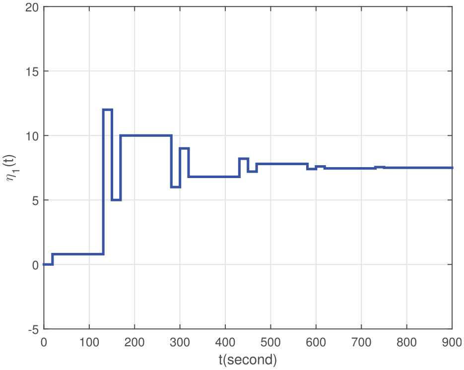
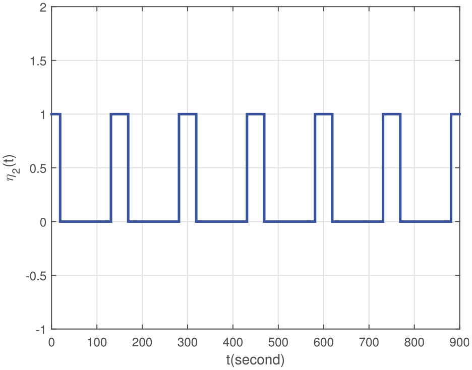
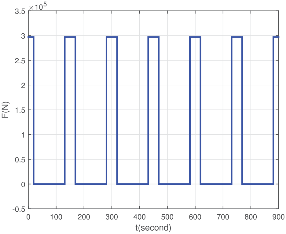
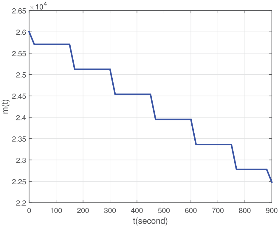
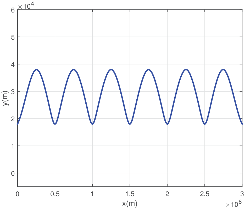
Following that, we solve the hypersonic vehicle optimal flight control problem by using Algorithm 1. The optimal value obtained is $J^{*}=3.4425\times {10}^{6}m$ . The value of the elevator deflection angle ${\eta }_1\left(t\right)$ , the throttle opening ${\eta }_2\left(t\right)$ , and the mass of the hypersonic vehicle $m\left(t\right)$ at the terminal time $t_f$ are ${\eta }_1\left(t_f\right)=7.5160$ , ${\eta }_2\left(t_f\right)=1.0000$ , $m\left(t_f\right)=2.2483\times {10}^4$ , respectively; The optimal elevator deflection angle ${\eta }_1\left(t\right)$ and the optimal throttle opening ${\eta }_2\left(t\right)$ are shown in Figures 1 and 2, respectively. The optimal trajectory of the engine thrust $F\left(t\right)$ , the optimal trajectory of the mass change for the hypersonic vehicle $m\left(t\right)$ , and the optimal flight path $(x\left(t\right),y\left(t\right))$ are shown in Figures 3 to 5, respectively.

Figure 1.

The optimal elevator deflection angle: ${\eta }_1\left(t\right)$ .

Figure 2.

The optimal throttle opening: ${\eta }_2\left(t\right)$ .

Figure 3.

The optimal trajectory of the engine thrust: $F\left(t\right)$ .

Figure 4.

The optimal trajectory of the mass change for the hypersonic vehicle: $m\left(t\right)$ .

Figure 5.

The optimal flight path: $(x\left(t\right),y\left(t\right))$ .

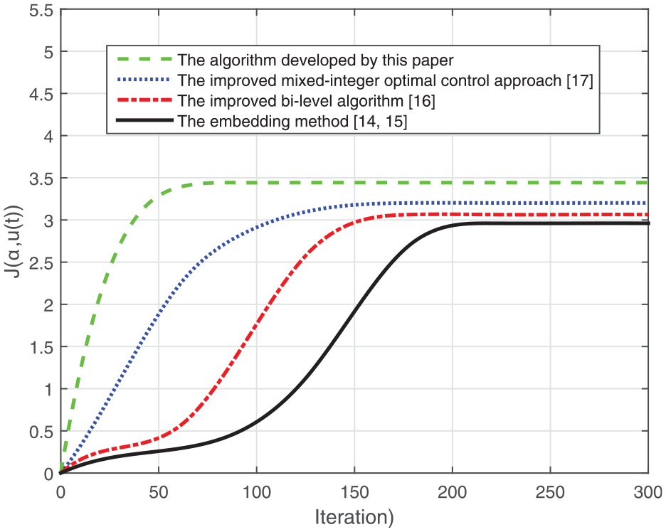
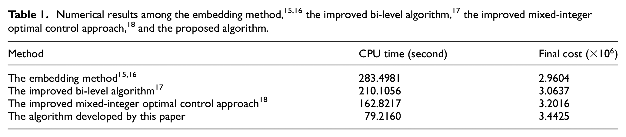
To compare with the existing approaches, the embedding approach,^15,16 the improved bi-level method, ¹⁷ and the improved mixed-integer optimal control approach ¹⁸ are used to show the solution of the above optimal problem with the same parameter. Numerical results are given by Figure 6 and Table 1. Figure 6 indicates that Algorithm 1 takes only 63 iterations to obtain a satisfactory value 3.4425, while the methods presented by Vasudevan et al., ¹⁵ Mei et al., ¹⁶ and Wu et al.^17,18 take 221 iterations, 187 iterations, and 152 iterations to obtain the satisfactory values 2.9604, 3.0637, and 3.2016, respectively. In other words, the iterations of Algorithm 1 are reduced by 71.5%, 56.1%, and 40.3%, respectively. Furthermore, compared with the methods presented by Vasudevan et al., ¹⁵ Mei et al., ¹⁶ and Wu et al.,^17,18 Table 1. also implies that Algorithm 1 can save 72.1%, 46.2%, and 29.5% computation time, respectively.

Figure 6.

Simulation of the embedding method,^15,16 the improved bi-level algorithm, ¹⁷ the improved mixed-integer optimal control approach, ¹⁸ and the proposed algorithm.

Table 1.

Numerical results among the embedding method,^15,16 the improved bi-level algorithm, ¹⁷ the improved mixed-integer optimal control approach, ¹⁸ and the proposed algorithm.

Method	CPU time (second)	Final cost ( $\times {10}^6$ )
The embedding method15,16	283.4981	2.9604
The improved bi-level algorithm 17	210.1056	3.0637
The improved mixed-integer optimal control approach 18	162.8217	3.2016
The algorithm developed by this paper	79.2160	3.4425

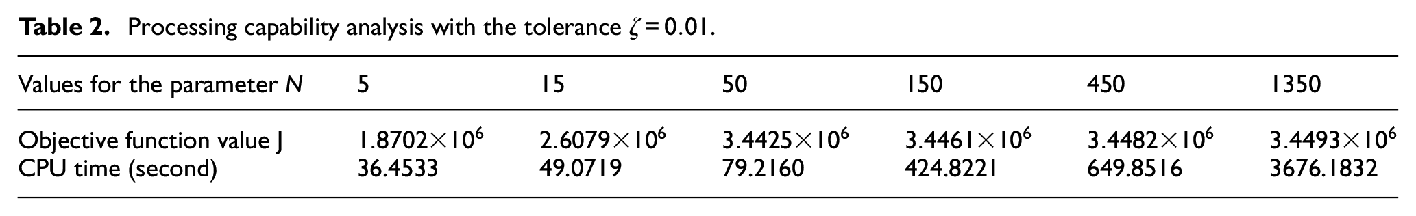
Theorems 4.1–4.2 provided by Goh and Teo ³² indicate that Problems 1 and 2 are equivalent as $N\to +\infty$ . Unfortunately, it is impossible to take a very large value of $N$ because of the limitation of computer accuracy. Following that, to demonstrate the effect of $N$ on the performance of the algorithm proposed by this paper, a sensitivity analysis for $N$ is performed and the numerical simulation results are presented by Table 2, which shows that the CPU time is also increasing as $N$ becomes larger. To balance the calculating cost and the accuracy of solutions, we set $N$ to $50$ . That is to say, a satisfactory solution can be achieved by using a finite value instead of a very large value of $N$ .

Table 2.

Processing capability analysis with the tolerance $\zeta =0.01$ .

Values for the parameter $N$	5	15	50	150	450	1350
Objective function value J	$1.8702\times {10}^6$	$2.6079\times {10}^6$	$3.4425\times {10}^6$	$3.4461\times {10}^6$	$3.4482\times {10}^6$	$3.4493\times {10}^6$
CPU time (second)	36.4533	49.0719	79.2160	424.8221	649.8516	3676.1832

For sensitivity analysis, let ${\omega }_1={\omega }_2=0.001$ , and the other parameters remain the same. Following that, we can obtain the effect of ${\omega }_1={\omega }_2=0.001$ in the constraints (62) and (63) on the cost function (12) by using the sensitivity analysis approach presented by the work. ³¹ The result is $\mathrm{\Delta }J=433.7550$ , which is only 0.0126% of the optimal value $J^{*}=3.4425\times {10}^6$ . This indicates that the cost function (12) is robust to the small disturbance in the constraints (62) and (63).

The above results indicate that the proposed algorithm is less time–consuming with faster convergence rate, and is better than the methods presented by the works.^15–18 That is, an alternative algorithm is proposed for the hypersonic vehicle optimal flight control problem. Furthermore, the results of sensitivity analysis imply that the cost function is robust to the small perturbation in the continuous-time inequality constraints.

Conclusion

A hypersonic vehicle optimal flight control problem is investigated in this paper. The hypersonic vehicle optimal flight control problem is modeled as a constrained OCPSS. Then, to achieve the globally optimal solution of the he hypersonic vehicle optimal flight control problem, we propose a penalty function-based improved CFF algorithm. Numerical results show that the proposed algorithm is effective and the cost function is robust to the small perturbation in the continuous-time inequality constraints.